Spin Relaxation in Quantum Wires
Abstract
The spin dynamics and spin relaxation of itinerant electrons in quantum wires with spin-orbit coupling is reviewed. We give an introduction to spin dynamics, and review spin-orbit coupling mechanisms in semiconductors. The spin diffusion equation with spin-orbit coupling is derived, using only intuitive, classical random walk arguments. We give an overview of all spin relaxation mechanisms, with particular emphasis on the motional narrowing mechanism in disordered conductors, the D’yakonov-Perel’-Spin relaxation (DPS). Here, we discuss in particular, the existence of persistent spin helix solutions of the spin diffusion equation, with vanishing spin relaxation rates. We then, derive solutions of the spin diffusion equation in quantum wires, and show that there is an effective alignment of the spin-orbit field in wires whose width is smaller than the spin precession length . We show that the resulting reduction in the spin relaxation rate results in a change in the sign of the quantum corrections to the conductivity. Finally, we present recent experimental results which confirm the decrease of the spin relaxation rate in wires whose width is smaller than : the direct optical measurement of the spin relaxation rate, as well as transport measurements, which show a dimensional crossover from weak antilocalization to weak localization as the wire width is reduced. Open problems remain, in particular in narrower, ballistic wires, were optical and transport measurements seem to find opposite behavior of the spin relaxation rate: enhancement, suppression, respectively. We conclude with a review of these and other open problems which still challenge the theoretical understanding and modeling of the experimental results.
I Introduction
The emerging technology of spintronics intends to use the manipulation of the spin degree of freedom of individual electrons for energy efficient storage and transport of information.[1] In contrast to classical electronics, which relies on the steering of charge carriers through semiconductors, spintronics uses the spin carried by electrons, resembling tiny spinning tops. The difference to a classical top is that its angular momentum is quantized, it can only take two discrete values, up or down. To control the spin of electrons, a detailed understanding of the interaction between the spin and orbital degrees of freedom of electrons and other mechanisms which do not conserve its spin, is necessary. These are typically weak perturbations, compared to the kinetic energy of conduction electrons, so that their spin relaxes slowly to the advantage of spintronic applications. The relaxation, or depolarization of the electron spin can occur due to the randomization of the electron momentum by scattering from impurities, and dislocations in the material, and due to scattering with elementary excitations of the solid such as phonons and other electrons, when it is transferred to the randomization of the electron spin due to the spin-orbit interaction. In addition, scattering from localized spins, such as nuclear spins and magnetic impurities are sources of electron spin relaxation. The electron spin relaxation can be reduced by constraining the electrons in low dimensional structures, quantum wells (confined in one direction, free in two dimensions), quantum wires ( confined in two directions, free in one direction), or quantum dots ( confined in all three directions). Although spin relaxation is typically smallest in quantum dots due to their discrete energy level spectrum, the necessity to transfer the spin in spintronic devices, recently lead to intense research efforts to reduce the spin relaxation in quantum wires, where the energy spectrum is continuous. In the following we will review the theory of spin dynamics and relaxation in quantum wires, and compare it with recent experimental results. After a general introduction to spin dynamics in Section II, we discuss all relevant spin relaxation mechanisms and how they depend on dimension, temperature, mobility, charge carrier density and magnetic field in Section III. In particular, we review recent results on spin relaxation in semiconducting quantum wires, and its influence on the quantum corrections to their conductance in Section IV. These weak localization corrections are thereby a very sensitive measure of spin relaxation in quantum wires, in addition to optical methods as we review in Section V. We set in the following.
II Spin Dynamics
Before we review the spin dynamics of conduction electrons and holes in semiconductors and metals, let us first reconsider the spin dynamics of a localized spin, as governed by the Bloch equations.
II.1 Dynamics of a Localized Spin
A localized spin , like a nuclear spin, or the spin of a magnetic impurity in a solid, precesses in an external magnetic field due to the Zeeman interaction with Hamiltonian , where is the corresponding gyromagnetic ratio of the nuclear spin or magnetic impurity spin, respectively, which we will set equal to one, unless needed explicitly. This spin dynamics is governed by the Bloch equation of a localized spin,
| (1) |
This equation is identical to the Heisenberg equation for the quantum mechanical spin operator of an -spin, interacting with the external magnetic field due to the Zeeman interaction with Hamiltonian . The solution of the Bloch equation for a magnetic field pointing in the z-direction is , while the x- and y- components of the spin are precessing with frequency around the z-axis, , . Since a localized spin interacts with its environment by exchange interaction and magnetic dipole interaction, the precession will dephase after a time , and the z-component of the spin relaxes to its equilibrium value within a relaxation time . This modifies the Bloch equations to the phenomenological equations,
| (2) |
II.2 Spin Dynamics of Itinerant Electrons
II.2.1 Ballistic Spin Dynamics
The intrinsic degree of freedom spin is a direct consequence of the Lorentz invariant formulation of quantum mechanics. Expanding the relativistic Dirac equation in the ratio of the electron velocity and the constant velocity of light , one obtains in addition to the Zeeman term, a term which couples the spin with the momentum of the electrons, the spin-orbit coupling
| (3) |
where we set the gyromagnetic ratio . , is an electrical field, and . Substitution into the Heisenberg equation yields the Bloch equation in the presence of spin-orbit interaction:
| (4) |
so that the spin performs a precession around the momentum dependent spin-orbit field . It is important to note, that the spin-orbit field does not break the invariance under time reversal ( ), in contrast to an external magnetic field . Therefore, averaging over all directions of momentum, there is no spin polarization of the conduction electrons. However, injecting a spin-polarized electron with given momentum into a translationally invariant wire, its spin precesses in the spin-orbit field as the electron moves through the wire. The spin will be oriented again in the initial direction after it moved a length , the spin precession length. The precise magnitude of does not only depend on the strength of the spin-orbit interaction but may also depend on the direction of its movement in the crystal, as we will discuss below.
II.2.2 Spin Diffusion Equation
Translational invariance is broken by the presence of disorder due to impurities and lattice imperfections in the conductor. As the electrons scatter from the disorder potential elastically, their momentum changes in a stochastic way, resulting in diffusive motion. That results in a change of the the local electron density , where denotes the orientation of the electron spin, and is the position and time dependent electron wave function amplitude. On length scales exceeding the elastic mean free path , that density is governed by the diffusion equation
| (5) |
where the diffusion constant is related to the elastic scattering time by , where is the Fermi velocity, and the Diffusion dimension of the electron system. That diffusion constant is related to the mobility of the electrons, by the Einstein relation , where is the density of states per spin at the Fermi energy . Injecting an electron at position into a conductor with previously constant electron density , the solution of the diffusion equation yields that the electron density spreads in space according to , where is the dimension of diffusion. That dimension is equal to the kinetic dimension , , if the elastic mean free path is smaller than the size of the sample in all directions. If the elastic mean free path is larger than the sample size in one direction the diffusion dimension reduces by one, accordingly. Thus, on average the variance of the distance the electron moves after time is . This introduces a new length scale, the diffusion length . We can rewrite the density as where is the two-component vector of the up (+), and down (-) spin fermionic creation operators, and the 2-component vector of annihilation operators, respectively, denotes the expectation value. Accordingly, the spin density is expected to satisfy a diffusion equation, as well. The spin density is defined by
| (6) |
where is the vector of Pauli matrices,
Thus the z-component of the spin density is half the difference between the density of spin up and down electrons, , which is the local spin polarization of the electron system. Thus, we can directly infer the diffusion equation for , and, similarly, for the other components of the spin density, yielding, without magnetic field and spin-orbit interaction,[2]
| (7) |
Here, in the spin relaxation term we introduced the tensor , which can have non-diagonal matrix elements. In the case of a diagonal matrix, , is the spin dephasing time, and the spin relaxation time. The spin diffusion equation can be written as a continuity equation for the spin density vector, by defining the spin diffusion current of the spin components ,
| (8) |
Thus, we get the continuity equation for the spin density components ,
| (9) |
II.2.3 Spin-Orbit Interaction in Semiconductors
While silicon and germanium have in their diamond structure an inversion symmetry around every midpoint on each line connecting nearest neighbor atoms, this is not the case for III-V-semiconductors like GaAs, InAs, InSb, or ZnS. These have a zinc-blende structure which can be obtained from a diamond structure with neighbored sites occupied by the two different elements. Therefore the inversion symmetry is broken, which results in spin-orbit coupling. Similarly, that symmetry is broken in II-VI-semiconductors. This bulk inversion asymmetry (BIA) coupling, or often so called Dresselhaus-coupling, is anisotropic, as given by [3]
| (10) |
where is the Dresselhaus-spin-orbit coefficient. Confinement in quantum wells with width on the order of the Fermi wave length yields accordingly a spin-orbit interaction where the momentum in growth direction is of the order of . Because of the anisotropy of the Dresselhaus term, the spin-orbit interaction depends strongly on the growth direction of the quantum well. Grown in direction, one gets, taking the expectation value of Eq. (10) in the direction normal to the plane, noting that , [3]
| (11) |
where is the linear Dresselhaus parameter. Thus, inserting an electron with momentum along the x-direction, with its spin initially polarized in z-direction, it will precess around the x-axis as it moves along. For narrow quantum wells, where the linear term exceeds the cubic Dresselhaus terms. A special situation arises for quantum wells grown in the - direction, where it turns out that the spin-orbit field is pointing normal to the quantum well, as shown in Fig. 1, so that an electron whose spin is initially polarized along the normal of the plane, remains polarized as it moves in the quantum well.
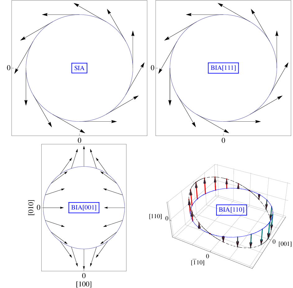
In quantum wells with asymmetric electrical confinement the inversion symmetry is broken as well. This structural inversion asymmetry (SIA) can be deliberately modified by changing the confinement potential by application of a gate voltage. The resulting spin-orbit coupling, the SIA coupling, also called Rashba-spin-orbit interaction[4] is given by
| (12) |
where depends on the asymmetry of the confinement potential in the direction , the growth direction of the quantum well, and can thus be deliberately changed by application of a gate potential. At first sight it looks as if the expectation value of the electrical field in the conduction band state vanishes, since the ground state of the quantum well must be symmetric in . Taking into account the coupling to the valence band,[5, 6] the discontinuities in the effective mass,[7] and corrections due to the coupling to odd excited states,[8] yields a sizable coupling parameter depending on the asymmetry of the confinement potential[6, 9].
This dependence allows one, in principle, to control the electron spin with a gate potential, which can therefore be used as the basis of a spin transistor.[10]
We can combine all spin-orbit couplings by introducing the spin-orbit field such that the Hamiltonian has the form of a Zeeman term:
| (13) |
where the spin vector is . But we stress again that since under the time reversal operation, spin-orbit coupling does not break time reversal symmetry, since the time reversal operation also changes the sign of the spin, . Only an external magnetic field breaks the time reversal symmetry. Thus, the electron spin operator is for fixed electron momentum governed by the Bloch equations with the spin-orbit field,
| (14) |
The spin relaxation tensor is no longer necessarily diagonal in the presence of spin-orbit interaction.
In narrow quantum wells where the cubic Dresselhaus coupling is weak compared to the linear Dresselhaus and Rashba couplings, the spin-orbit field is given by
| (15) |
which changes both its direction and its amplitude , as the direction of the momentum is changed. Accordingly, the electron energy dispersion close to the Fermi energy is in general anisotropic as given by
| (16) |
where , , and . Thus, when an electron is injected with energy , with momentum along the -direction, , its wave function is a superposition of plain waves with the positive momenta . The momentum difference causes a rotation of the electron eigenstate in the spin subspace. When at the electron spin was polarized up spin, with the Eigenvector
then, when its momentum points in x-direction, at a distance , it will have rotated the spin as described by the Eigenvector
| (17) |
In Fig. 2 we plot the corresponding spin density as defined in Eq. (6) for pure Rashba coupling, .

The spin will point again in the initial direction, when the phase difference between the two plain waves is , which gives the condition for spin precession length as , yielding for linear Rashba and Dresselhaus coupling, and the electron moving in - direction,
| (18) |
We note that the period of spin precession changes with the direction of the electron momentum since the spin-orbit field, Eq. (15), is anisotropic.
II.2.4 Spin Diffusion in the Presence of Spin-Orbit Interaction
As the electrons are scattered by imperfections like impurities and dislocations, their momentum is changed randomly. Accordingly, the direction of the spin-orbit field changes randomly as the electron moves through the sample. This has two consequences: the electron spin direction becomes randomized, dephasing the spin precession and relaxing the spin polarization. In addition, the spin precession term is modified, as the momentum changes randomly, and has no longer the form given in the ballistic Bloch-like equation, Eq. (14). One can derive the diffusion equation for the expectation value of the spin, the spin density Eq. (6) semiclassically, [11, 12] or by diagrammatic expansion.[13] In order to get a better understanding on the meaning of this equation, we will give a simplified classical derivation, in the following. The spin density at time can be related to the one at the earlier time . Note that for ballistic times , the distance the electron has moved with a probability , , is related to that time by the ballistic equation, when the electron moves with the momentum . On this time scale the spin evolution is still governed by the ballistic Bloch equation Eq. (14). Thus, we can relate the spin density at the position at the time , to the one at the earlier time at position :
| (19) |
Now, we can expand in to first order and in to second order. Next, we average over the disorder potential, assuming that the electrons are scattered isotropically, and substitute where is the total angle, and denotes the integral over all angles with . Also, we get for , and , where is the diffusion constant. While the disorder average yields , and , separately, for isotropic impurity scattering, averaging their product yields a finite value, since depends on the momentum at time , , yielding , where denotes the average over the Fermi surface. This way, we can also evaluate the average of the spin-orbit term in Eq. (19), expanded to first order in , and get, substituting the spin diffusion equation,
| (20) |
where denotes the average over the Fermi surface. Spin polarized electrons injected into the sample spread diffusively, and their spin polarization, while spreading diffusively as well, decays in amplitude exponentially in time. Since, between scattering events the spins precess around the spin-orbit fields, one expects also an oscillation of the polarization amplitude in space. One can find the spatial distribution of the spin density which is the solution of Eq. (20) with the smallest decay rate . As an example, the solution for linear Rashba coupling is, [12]
| (21) |
with where and where the amplitude of the momentum is determined by , and , and . This solution is plotted in Fig. 3 for . In Fig. 4 we plot the linearly independent solution obtained by interchanging and in Eq. (21), with the spin pointing in z-direction, initially. We choose . Comparison with the ballistic precession of the spin, Fig 4 shows that the period of precession is enhanced by the factor in the diffusive wire, and that the amplitude of the spin density is modulated, changing from to .


Injecting a spin-polarized electron at one point, say , its density spreads the same way it does without spin-orbit interaction, , where is the distance to the injection point. However, the decay of the spin density is periodically modulated as a function of .[14] The spin-orbit interaction together with the scattering from impurities is also a source of spin relaxation, as we discuss in the next Section together with other mechanisms of spin relaxation. We can find the classical spin diffusion current in the presence of spin-orbit interaction, in a similar way as one can derive the classical diffusion current: The current at the position is a sum over all currents in its vicinity which are directed towards that position. Thus, where an angular average over all possible directions of the velocity is taken. Expanding in , and noting that , one gets . For the classical spin diffusion current of spin component , as defined by , there is the complication that the spin keeps precessing as it moves from to , and that the spin-orbit field changes its direction with the direction of the electron velocity . Therefore, the 0-th order term in the expansion in does not vanish, rather, we get , where is the part of the spin density which evolved from the spin density at moving with velocity and momentum . Noting that the spin precession on ballistic scales is governed by the Bloch equation, Eq. (14), we find by integration of Eq. (14), that so that we can rewrite the first term yielding the total spin diffusion current as
| (22) |
Thus, we can rewrite the spin diffusion equation in terms of this spin diffusion current and get the continuity equation
| (23) |
It is important to note that in contrast to the continuity equation for the density, there are two additional terms, due to the spin orbit interaction. The last one is the spin relaxation tensor which will be considered in detail in the next section. The other term arises due to the fact that Eq. (20) contains a factor in front of the spin-orbit precession term, while the spin diffusion current Eq. (22) does not contain that factor. This has important physical consequences, resulting in the suppression of the spin relaxation rate in quantum wires and quantum dots as soon as their lateral extension is smaller than the spin precession length , as we will see in the subsequent Sections.
III Spin Relaxation Mechanisms
The intrinsic spin-orbit interaction itself causes the spin of the electrons to precess coherently, as the electrons move through a conductor, defining the spin precession length , Eq. (18). Since impurities and dislocations in the conductor randomize the electron momentum, the impurity scattering is transferred into a randomization of the electron spin by the spin-orbit interaction, which thereby results in spin dephasing and spin relaxation. This results in a new length scale, the spin relaxation length, , which is related to the spin relaxation rate by
| (24) |
III.1 D’yakonov-Perel’ Spin Relaxation
D’yakonov-Perel’ spin relaxation (DPS) can be understood qualitatively in the following way: The spin-orbit field changes its direction randomly after each elastic scattering event from an impurity, that is, after a time of the order of the elastic scattering time , when the momentum is changed randomly as sketched in Fig. 5.

Thus, the spin has the time to perform a precession around the present direction of the spin-orbit field, and can thus change its direction only by an angle of the order of by precession. After a time with scattering events, the direction of the spin will therefore have changed by an angle of the order of . Defining the spin relaxation time as the time by which the spin direction has changed by an angle of order one, we thus find that , where the angular brackets denote integration over all angles. Remarkably, this spin relaxation rate becomes smaller, the more scattering events take place, because the smaller the elastic scattering time is, the less time the spin has to change its direction by precession. Such a behavior is also well known as motional, or dynamic narrowing of magnetic resonance lines.[15] A more rigorous derivation for the kinetic equation of the spin density matrix yields additional interference terms, not taken into account in the above argument. It can be obtained by iterating the expansion of the spin density Eq. (19) once in the spin precession term, which yields the term
| (25) |
where denotes the average over all angles due to the scattering
from impurities. Since the electrons move ballistically at times smaller than
the elastic scattering time, the momenta are correlated only on time scales smaller
than , yielding .
Noting that and we find that
Eq. (25) simplifies to ,
where the matrix elements of the spin relaxation terms are given by,
[16]
| (26) |
where denotes the average over the direction of the momentum . These non-diagonal terms can diminish the spin relaxation and even result in vanishing spin relaxation. As an example, we consider a quantum well where the linear Dresselhaus coupling for quantum wells grown in direction, Eq. (11), and linear Rashba-coupling, Eq. (12), are the dominant spin-orbit couplings. The energy dispersion is anisotropic, as given by Eq. (16), and the spin-orbit field changes its direction and its amplitude with the direction of the momentum :
| (27) |
with . Thus we find the spin relaxation tensor as,
| (28) |
Diagonalizing this matrix, one finds the three eigenvalues and where , and . Note, that one of these eigenvalues of the spin relaxation tensor vanishes when . In fact, this is a special case, when the spin-orbit field does not change its direction with the momentum:
| In this case the constant spin density given by | ||||
does not decay in time, since the spin density vector is parallel to the spin orbit field , Eq. (III.1), and cannot precess, as has been noted in Ref. [17]. It turns out, however, that there are two more modes which do not decay in time, whose spin relaxation rate vanishes for . These modes are not homogeneous in space, and correspond to precessing spin densities. They were found previously in a numerical Monte Carlo simulation and found not to decay in time, being called therefore persistent spin helix.[18, 19] Recently, a long living inhomogeneous spin density distribution has been detected experimentally in Ref. [20]. We can now get these persistent spin helix modes analytically, by solving the full spin diffusion equation Eq. (20) with the spin relaxation tensor given by Eq. (28). We can diagonalize that equation, noting that its eigenfunctions are plain waves . Thereby one finds, first of all, the mode with Eigenvalue , with the spin density
| (35) |
Indeed for , the homogeneous solution, it does not decay in time, in agreement with the solution we found above, Eq. (35). There are, however, two more modes with the eigenvalues
| (36) |
where . At , these modes do not decay in time. These two stationary solutions, are
| (37) |
and the linearly independent solution, obtained by interchanging and in Eq. (37). The spin precesses as the electrons diffuse along the quantum wire with the period , the spin precession length, forming a persistent spin helix, as shown in Fig. 6.

III.2 DP Spin Relaxation with Electron-Electron and Electron-Phonon Scattering
It has been noted, that the momentum scattering which limits the D’yakonov-Perel’ mechanism of spin relaxation is not restricted to impurity scattering, but can also be due to electron-phonon or electron-electron interactions.[21, 22, 23, 24] Thus the scattering time, is the total scattering time as defined by, [21, 22] , where is the elastic scattering rate due to scattering from impurities with potential , given by , where is the density of states per spin at the Fermi energy, is the concentration of impurities with potential , and . In degenerate semiconductors and in metals, the electron-electron scattering rate is given by the Fermi liquid inelastic electron scattering rate . The electron-phonon scattering time decays faster with temperature. Thus, at low temperatures the DP spin relaxation is dominated by elastic impurity scattering .
III.3 Elliott-Yafet Spin Relaxation
Because of the spin-orbit interaction the conduction electron wave functions are not Eigenstates of the electron spin, but have an admixture of both spin up and spin down wave functions. Thus, a nonmagnetic impurity potential can change the electron spin, by changing their momentum due to the spin-orbit coupling. This results in another source of spin relaxation which is stronger, the more often the electrons are scattered, and is thus proportional to the momentum scattering rate .[25, 26] For degenerate III-V semiconductors one finds[27, 28]
| (38) |
where is the gap between the valence and the conduction band of the semiconductor, the energy of the conduction electron, and is the spin-orbit splitting of the valence band. Thus, the Elliott-Yafet spin relaxation (EYS) can be distinguished, being proportional to , and thereby to the resistivity, in contrast to the DP spin scattering rate, Eq. (26), which is proportional to the conductivity. Since the EYS decays in proportion to the inverse of the band gap, it is negligible in large band gap semiconductors like and . The scattering rate is again the sum of the impurity scattering rate,[25] the electron-phonon scattering rate,[26, 29] and electron-electron interaction, [30] so that all these scattering processes result in EYS. In non-degenerate semiconductors, where the Fermi energy is below the conduction band edge, attains a stronger temperature dependence.
III.4 Spin Relaxation due to Spin-Orbit Interaction with Impurities
The spin-orbit interaction, as defined in Eq. (3), arises whenever there is a gradient in an electrostatic potential. Thus, the impurity potential gives rise to the spin-orbit interaction
| (39) |
Perturbation theory yields then directly the corresponding spin relaxation rate
| (40) |
proportional to the concentration of impurities . Here denotes the spin indices. Since the spin-orbit interaction increases with the atomic number of the impurity element, this spin relaxation increases as , being stronger for heavier element impurities.
III.5 Bir-Aronov-Pikus Spin Relaxation
The exchange interaction between electrons and holes in p-doped semiconductors results in spin relaxation, as well.[31, 32] Its strength is proportional to the density of holes and depends on their itinerancy. If the holes are localized they act like magnetic impurities. If they are itinerant, the spin of the conduction electrons is transferred by the exchange interaction to the holes, where the spin-orbit splitting of the valence bands results in fast spin relaxation of the hole spin due to the Elliott-Yafet, or the D’yakonov-Perel’ mechanism.
III.6 Magnetic Impurities
Magnetic impurities have a spin which interacts with the spin of the conduction electrons by the exchange interaction , resulting in a spatially and temporarily fluctuating local magnetic field
| (41) |
where the sum is over the position of the magnetic impurities . This gives rise to spin relaxation of the conduction electrons, with a rate given by
| (42) |
where is the density of magnetic impurities, and is the density of states at the Fermi energy. Here, is the spin quantum number of the magnetic impurity, which can take the values . Antiferromagnetic exchange interaction between the magnetic impurity spin and the conduction electrons results in a competition between the conduction electrons to form a singlet with the impurity spin, which results in enhanced nonmagnetic and magnetic scattering. At low temperatures the magnetic impurity spin is screened by the conduction electrons resulting in a vanishing of the magnetic scattering rate. Thus, the spin scattering from magnetic impurities has a maximum at a temperature of the order of the Kondo temperature , where is the density of states at the Fermi energy.[33, 34, 35] In semiconductors is exponentially small due to the small effective mass and the resulting small density of states . Therefore, the magnetic moments remain free at the experimentally achievable temperatures. At large concentration of magnetic impurities, the RKKY-exchange interaction between the magnetic impurities quenches however the spin quantum dynamics, so that is replaced by its classical value . In Mn-p-doped GaAs, the exchange interaction between the Mn dopants and the holes can result in compensation of the hole spins and therefore a suppression of the Bir-Aronov-Pikus (BAP) spin relaxation.[36]
III.7 Nuclear Spins
Nuclear spins interact by the hyperfine interaction with conduction electrons. The hyperfine interaction between nuclear spins and the conduction electron spin, , results in a local Zeeman field given by [37]
| (43) |
where is the gyromagnetic ratio of the nuclear spin. The spatial and temporal fluctuations of this hyperfine interaction field result in spin relaxation proportional to its variance, similar to the spin relaxation by magnetic impurities.
III.8 Magnetic Field Dependence of Spin Relaxation
The magnetic field changes the electron momentum due to the Lorentz force, resulting in a continuous change of the spin-orbit field, which similar to the momentum scattering results in motional narrowing and thereby a reduction of DPS: [38, 39, 28, 40]
| (44) |
Another source of a magnetic field dependence is the precession around the external magnetic field. In bulk semiconductors and for magnetic fields perpendicular to a quantum well, the orbital mechanism is dominating, however. This magnetic field dependence can be used to identify the spin relaxation mechanism, since the EYS does have only a weak magnetic field dependence due to the weak Pauli-paramagnetism.
III.9 Dimensional Reduction of Spin Relaxation
Electrostatic confinement of conduction electrons can reduce the effective dimension of their motion. In quantum dots, the electrons are confined in all three directions, and the energy spectrum consists of discrete levels like in atoms. Therefore, the energy conservation restricts relaxation processes severely, resulting in strongly enhanced spin relaxation times in quantum dots.[41, 42] Then, spin relaxation can only occur due to absorption or emission of phonons, yielding spin relaxation rates proportional to the inelastic electron-phonon scattering rate.[41] Quantitative comparison of the various spin relaxation mechanisms in GaAs quantum dots resulted in the conclusion that the spin relaxation is dominated by the hyperfine interaction.[43, 44, 45] A similar conclusion can be drawn from experiments on low temperature spin relaxation in low density n-type GaAs, where the localization of the electrons in the impurity band results in spin relaxation dominated by hyperfine interaction as well.[46, 47] For linear Rashba and linear Dresselhaus spin-orbit coupling we can see from the spin diffusion equation Eq. (20) with the DP spin relaxation tensor Eq. (28) that the spin relaxation vanishes, when the spin current Eq. (22) vanishes, in which case the last two terms of Eq. (20) cancel exactly. The vanishing of the spin current is imposed by hard wall boundary condition for which the spin diffusion current vanishes at the boundaries of the sample, , where is the normal to the boundary. When the quantum dot is smaller than the spin precession length the lowest energy mode thus corresponds to a homogeneous solution with vanishing spin relaxation rate. Cubic spin-orbit coupling does not yield such a vanishing of the DP spin relaxation rate. Only in quantum dots whose size does not exceed the elastic mean free path the DP spin relaxation from cubic spin relaxation becomes diminished. In quantum wires, the electrons have a continuous spectrum of delocalized states. Still, transverse confinement can reduce the DP spin relaxation as we review in the next section.
IV Spin-Dynamics in Quantum Wires
IV.1 One-Dimensional Wires
In one dimensional wires, whose width is of the order of the Fermi wave length , impurities can only reverse the momentum . Therefore, the spin-orbit field can only change its sign, when a scattering from impurities occurs. . Therefore, the precession axis and the amplitude of the spin orbit field does not change, reversing only the spin precession, so that the D’yakonov-Perel’-spin relaxation is absent in one dimensional wires.[48] In an external magnetic field, the precession around the magnetic field axis, due to the Zeeman-interaction is competing with the spin-orbit field, however. Then, as the electrons are scattered from impurities, both the precession axis and the amplitude of the total precession field is changing, since
resulting in spin dephasing and relaxation, as the sign of the momentum changes randomly.
IV.2 Spin-Diffusion in Quantum Wires
How does the spin relaxation rate depend on the wire width when the quantum wire has more than one channel occupied, ? Clearly, for large wire widths, the spin relaxation rate should converge to a finite value, while it vanishes for . It is both of practical importance for spintronic applications and of fundamental interest to know on which length scales this crossover occurs. Basically, there are three intrinsic length scales characterizing the quantum wire relative to its width . The Fermi wave length , the elastic mean free path and the spin precession length , Eq. (18). Suppression of spin relaxation for wire widths not exceeding the elastic mean free path , has been predicted and obtained numerically in Refs. [49, 11, 50, 51, 52, 53]. Is the spin relaxation rate also suppressed in diffusive wires in which the elastic mean free path is smaller than the wire width as in the wire shown schematically in Fig. 7? We will answer this question by means of an analytical derivation in the following.

The transversal confinement imposes that the spin current vanishes normal to the boundary, . For a wire grown along the direction, is the unit vector in the -direction. For wire widths smaller than the spin precession length , the solutions with the lowest energy have thus a vanishing transverse spin current, and the spin diffusion equation Eq. (20) becomes
| (45) |
with
| (46) |
where is the width of the wire. One sees that this equation has a persistent solution, which does not decay in time and is homogeneous along the wire, . In this special case the spin diffusion equation simplifies to[12]
| (47) |
Indeed this has one persistent solution given by
| (48) |
Thus, we can conclude that the boundary conditions impose an effective alignment of all spin-orbit fields, in a direction identical to the one it would attain in a one-dimensional wire, along the [010]-direction, setting in Eq. (27),
| (49) |
which therefore does not change its direction when the electrons are scattered. This is remarkable, since this alignment already occurs in wires with many channels, where the impurity scattering is two-dimensional, and the transverse momentum actually can be finite. Rather, the alignment of the spin-orbit field, accompanied by a suppression of the DP spin relaxation rate occurs due to the constraint on the spin-dynamics imposed by the boundary conditions as soon as the wire width is smaller than the length scale which governs the spin dynamics, namely, the spin precession length . It turns out that the spin diffusion equation Eq. (45) has also two long persisting spin helix solutions in narrow wires[54, 13] which oscillate periodically with the period . In contrast to the situation in 2D systems we reviewed in the previous Section, in quantum wires of width these solutions are long persisting even for . These two stationary solutions, are
| (50) |
and the linearly independent solution, obtained by interchanging and in Eq. (50). The spin precesses as the electrons diffuse along the quantum wire with the period , the spin precession length, forming a persistent spin helix, whose x-component is proportional to the linear Dresselhaus-coupling while its y-component is proportional to the Rashba-coupling as seen in Fig. 8.

A similar reduction of the spin relaxation rate is not effective for cubic spin-orbit coupling for wire widths exceeding the elastic mean free path . One can derive the spin relaxation rate as function of the wire width for diffusive wires . The total spin relaxation rate, in the presence of both linear Rashba spin-orbit coupling and linear and cubic Dresselhaus coupling , and , is as function of wire width given by,[54]
| (51) |
where . We introduced the dimensionless factor, with where depends on Dresselhaus spin-orbit coupling, . depends on Rashba coupling: . Thus, for negligible cubic Dresselhaus spin-orbit coupling the the spin relaxation length increases when decreasing the wire width as,
| (52) |
This can be understood as follows: [55, 56, 54] In a wire whose width exceeds the spin precession length , the area an electron covers by diffusion in time is . To achieve spin relaxation, this area should be equal to the corresponding 2D spin relaxation area , where . Thus, the smaller the wire width, the larger the spin relaxation length becomes, in agreement with Eq. (52). For larger wire widths, the spin diffusion equation can be solved as well, and one finds that the spin relaxation rate does not increase monotonously to the 2D limiting value but shows oscillations on the scale , which can be understood in analogy to Fabry-Pérot resonances.[54] For pure linear Rashba coupling that behavior can be derived analytically, in the approximation of a homogeneous spin density in transverse direction, yielding a relaxation rate given by
| (53) |
where . Furthermore, taking into account the transverse modulation of the spin density by performing an exact diagonalization of the spin diffusion equation with the transverse boundary conditions, Eq. (46), one finds for modes which are localized at the boundaries and have a lower relaxation rate than the bulk modes.[12, 13] For pure Rashba spin relaxation we find that there is a spin-helix solution located at the edge whose relaxation rate is smaller than the spin relaxation rate of bulk modes .
IV.3 Weak Localization Corrections
Quantum interference of electrons in low-dimensional, disordered conductors results in corrections to the electrical conductivity . This quantum correction, the weak localization effect, is known to be a very sensitive tool to study dephasing and symmetry breaking mechanisms in conductors.[57, 58, 59] The entanglement of spin and charge by spin-orbit interaction reverses the effect of weak localization and thereby enhances the conductivity, the weak antilocalization effect. The quantum correction to the conductivity arises from the fact, that the quantum return probability to a given point after a time , , differs from the classical return probability, due to quantum interference. As the electrons scatter from impurities, there is a finite probability that they diffuse on closed paths, which does increase the lower the dimension of the conductor. Since an electron can move on such a closed orbit clockwise or anticlockwise as shown in light and dark blue in Fig. 9, with equal probability, the probability amplitudes of both paths add coherently, if their length is smaller than the dephasing length .


In a magnetic field, indicated by the
red arrow in the middle Fig. 9, the electrons acquire a magnetic
flux phase. This phase depends on the direction in which the electron moves on the
closed path. Thus, the quantum interference is
diminished in an external magnetic field since the area of closed paths and thereby the flux
phases are randomly distributed
in a disordered wire, even though the magnetic field can be constant.
Similarly, the scattering from magnetic impurities breaks the time reversal invariance
between the two directions in which the closed path can be transversed. Therefore
magnetic impurities diminish
the quantum corrections in proportion to the rate with which the electron spins
scatter from them due to the exchange interaction, , Eq. (42).
Thus, the quantum correction to the conductivity, is proportional to the integral over all times smaller than the dephasing time of the quantum mechanical return probability , where is dimension of diffusion, and is the electron density. In the presence of spin-orbit scattering, the sign of the quantum correction changes to weak antilocalization as was as predicted by Hikami, Larkin, and Nagaoka [60] for conductors with impurities of heavy elements. As conduction electrons scatter from such impurities, the spin-orbit interaction randomizes their spin, Fig. 10.

The resulting spin relaxation suppresses interference of time reversed paths in spin triplet configurations, while interference in singlet configuration remains unaffected as indicated in Fig. 10. Since singlet interference reduces the electron’s return probability it enhances the conductivity, the weak antilocalization effect. Weak magnetic fields suppress also these singlet contributions, reducing the conductivity and resulting in negative magnetoconductivity. If the host lattice of the electrons provides spin-orbit interaction, the spin relaxation of DP or EY type does have the same effect of diminishing the quantum corrections in the triplet configuration. When the dephasing length is smaller than the wire width , the quantum corrections are determined by the interference of 2-dimensional closed diffusion paths, and as a result, the conductivity increases logarithmically with which increases itself as the temperature is lowered. At low temperatures, the electron-electron scattering is the dominating mechanism of spin dephasing, yielding . One can derive the magnetic field dependence of that quantum correction nonperturbatively.[60, 61, 62, 42, 63, 64] An approximate expression showing the logarithmic dependence explicitly is given by
| (54) |
in units of . All parameters are rescaled to dimensions of magnetic fields: , , the spin relaxation field due to spin orbit relaxation, ,[61] and the spin relaxation field due to magnetic impurities . Here is the DP relaxation rate in the 2D limit derived in the previous section. [61, 65] The prefactor depends on the particular spin-orbit interaction. For linear Rashba-coupling, . Note that is the smallest spin relaxation rate of an inhomogeneous spin density distribution[13] as derived in the section II.2.4. is the magnetic scattering rate from magnetic impurities, Eq. (42). Indeed we see that the first term does not depend on the DP spin relaxation rate. This term originates from the interference of time reversed paths, indicated in Fig. 10, which contributes to the quantum conductance in the singlet state, , the minus sign in front of the second term is the origin of the change in sign in the weak localization correction. The other three terms are suppressed by the spin relaxation rate, since they originate from interference in triplet states, which do not conserve the spin symmetry. Thus, at strong spin-orbit induced spin relaxation the last three terms are suppressed and the sign of the quantum correction switches to weak antilocalization. In quasi-1-dimensional quantum wires which are coherent in transverse direction, the weak localization correction is further enhanced, and increases linearly with the dephasing length . Thus, for the weak localization correction is [54]
| (55) |
in units of . We defined , and the effective external magnetic field,
| (56) |
The spin relaxation field is for ,
| (57) |
suppressed in proportion to . Taking one transverse mode into account the quantum conductivity correction is plotted in Fig. 11 for different wire withs for pure Rashba SOC, showing the crossover from weak localization (positive magnetoconductivity) to weak antilocalization (negative magnetoconductivity).

In analogy to the effective magnetic field, Eq. (56), the spin orbit coupling acts in quantum wires like an effective magnetic vector potential.[55] One can expect that in ballistic wires, , the spin relaxation rate is suppressed in analogy to the flux cancellation effect, which yields the weaker rate, , where .[66, 67, 68] A dimensional crossover from weak antilocalization to weak localization and a reduction of spin relaxation has recently been observed experimentally in quantum wires as we will review in the next Section.
V Experimental Results on Spin Relaxation Rate in Semiconductor Quantum Wires
V.1 Optical Measurements
Optical time-resolved Faraday rotation (TRFR) spectroscopy [69] has been used to probe the spin dynamics in an array of n-doped InGaAs wires by Holleitner et al. in Ref. [70, 71]. The wires were dry etched from a quantum well grown in the [001]-direction with a distance of 1 m between the wires. Spin aligned charge carriers were created by absorption of circularly-polarized light. For normal incidence, the spins point then perpendicular to the quantum well plane, in the growth direction [001]. The time evolution of the spin polarization was then measured with a linearly
polarized pulse, see inset of Fig. 1c of Ref. [70]. The
time dependence fits well with an exponential decay
. As seen in Fig. 2a of Ref. [70],
the thus measured lifetime at fixed temperature K of the spin polarization is enhanced when the wire
width is reduced[70]: While for m it is ps,
it increases for channels grown along the [100]- direction to almost ps,
and in the [110]- direction to about ps. Thus, the experimental results show that
the spin relaxation depends on the patterning direction of the
wires: wires aligned along [100] and [010] show
equivalent spin relaxation times, which are generally longer than
the spin relaxation times of wires patterned along [110] and
[10].
The dimensional reduction could be seen already
for wire widths as wide as m,
which is much wider than both the Fermi wave length and the elastic mean free path
in the wires. This agrees well with the predicted reduction of the DP scattering rate,
Eq. (51) for wire widths smaller than the spin precession length .
From the measured 2D spin diffusion length m, and its relation to the spin precession length Eq. (18), , we expect the crossover to occur on a scale of m as observed in Fig. 2a of Ref. [70].
From we get with a spin-orbit coupling
meVÅ.
According to
, the spin relaxation length increases by a factor of
in the [100]-, and by
in the [110]- direction.
The spin relaxation time has been found to attain a maximum, however, at about
, decaying appreciably for smaller widths.
While a saturation of could be expected according to Eq. (51)
for diffusive wires, due to cubic Dresselhaus-coupling,
a decrease is unexpected. Schwab et al., Ref. [12], noted that
with wire boundary conditions which do not conserve the spin of the conduction electrons
one can obtain such a reduction. A mechanism for such spin-flip processes
at the edges of the wire has not yet been identified, however.
The magnetic field dependence of the
spin relaxation rate yields further confirmation that the dominant
spin relaxation mechanism in these wires is DPS:
It follows the predicted behavior Eq. (44),
as seen in Fig. 3a of Ref. [70], and the spin relaxation rate is
enhanced to ps for all wire growth directions, at K
and wire widths of m.
V.2 Transport Measurements
A dimensional crossover from weak antilocalization to weak localization and a
reduction of spin relaxation has recently been observed experimentally in n-doped InGaAs quantum wires,[72, 73] in GaAs wires,[74] as well
as in AlGaN/GaN wires.[75]
The crossover indeed occurred in all experiments on the
length scale of the spin precession length .
We summarize in the following the main results of these experiments.
Wirthmann et al., Ref. [72], measured the magnetoconductivity
of inversion-doped InAs quantum wells
with a density of , and a measured effective mass of
. In the wide wires the magnetoconductivity showed a pronounced
weak antilocalization peak, which agreed well with the 2D theory, [65, 61]
with a spin-orbit-coupling parameter of meVÅ.
They observed a diminishment of the antilocalization peak
which occurred for wire widths
m, at K, indicating a dimensional reduction of the DP spin relaxation rate.
Schäpers et al. observed in GaxIn1-xAs/InP quantum wires a complete crossover from weak antilocalization to weak localization for wire widths below nm.
Such a crossover has also been observed in GaAs-quantum wires by Dinter et al., Ref. [74].
Very recently, Kunihashi et al., Ref. [76] observed the crossover from
weak antilocalization to weak localization in gate controlled InGaAs quantum wires.
The asymmetric potential normal to the quantum well
could be enhanced by application of a negative gate voltage, yielding an increase of the
SIA-coupling parameter , with decreasing carrier density,
as was obtained by fitting the magnetoconductivity of the quantum wells
to the theory of 2D weak localization corrections of Iordanskii et al., Ref. [65].
Thereby, the spin relaxation length
was found to decrease from m to m, which according to
corresponds to an increase of
from meVÅ at electron concentrations of
to meVÅ at electron concentrations of .
The magnetoconductivity of a sample with 95
quantum wires in parallel showed a clear crossover from weak antilocalization to
localization.
Fitting the data to Eq. (55) a corresponding decrease of the spin relaxation rate
was obtained, which was observable already at large widths of the order
of the spin precession length in agreement with the theory Eq. (51).
However, a saturation as obtained theoretically in diffusive wires,
due to cubic BIA-coupling was not observed. This might be due to the limitation of
Eq. (51), to diffusive wire widths, , while in ballistic wires
a suppression also of the spin relaxation due to cubic BIA-coupling can be expected,
since it vanishes identically in 1-D wires, see section IV.1.
Also, an increase of the spin scattering rate in narrower
wires, , was not observed in contrast to the
results of the optical experiments, Ref. [70],
reviewed above.
The dimensional crossover has also been observed in the heterostructures
of the wide gap semiconductor GaN.[75]
The magnetoconductivity of 160 AlGaN/GaN- quantum wires were measured.
The effective mass is , all wires were diffusive with .
For electron densities of an increase from
nm to m,
and for densities an increase from
nm to m was observed.
Using , one obtains
for both densities , the spin-orbit coupling meVÅ.
A saturation of the spin relaxation rate could not be observed,
suggesting that the cubic BIA-coupling is negligible in these structures.
We note, that an enhancement of the spin relaxation rate as in the optical experiments of narrow
InGaAs quantum wires, Ref. [70], was not observed in these
AlGaN/GaN-wires.
VI Critical Discussion and Future Perspective
The fact that optical and transport measurements seem to find opposite behavior, enhancement and suppression of the spin relaxation rate, respectively, in narrow wires, calls for an extension of the theory to describe the crossover to ballistic quantum wires. This can be done, using the kinetic equation approach to the spin-diffusion equation,[12] a semiclassical approach, [77, 78] or an extension of the diagrammatic approach.[13] In particular, the dimensional crossover of DPS due to cubic Dresselhaus coupling, which we found not to be suppressed in diffusive wires, needs to be studied for ballistic wires, , as many of the experimentally studied quantum wires are in this regime. Furthermore, using the spin diffusion equation, one can study the dependence on the growth direction of quantum wires, and find more information on the magnitude of the various spin-orbit coupling parameters, , by comparison with the directional dependence found in both the optical measurements[70] of the spin relaxation rate, as well as in recent gate controlled transport experiments.[76]
In narrow wires, corrections due to electron-electron interaction can become more important and influence especially the temperature dependence. Ref. [71] reports a strong temperature dependence of the spin relaxation rate in narrow quantum wires. As shown in Ref. [23], the spin relaxation rates obtained from the spin diffusion equation and the quantum corrections to the magnetoconductivity can be different, when corrections due to electron-electron interaction become important. As the DPS becomes suppressed in quantum wires other spin relaxation mechanisms like the EYS may become dominant, since it is expected that the dimensional dependence of EYS is less strong. In more narrow wires, disorder can also result in Anderson localization. Similar as in quantum dots, [41, 45] this can yield enhanced spin relaxation due to hyperfine coupling, Eq. (43). The spin relaxation in metal wires is believed to be dominated by the EYS mechanism, which is not expected to show such a strong wire width dependence, although this needs to be explored in more detail. Even dilute concentrations of magnetic impurities of less than 1 ppm, do yield measurable spin relaxation rates in metals and allow the study of the Kondo effect with unprecedented accuracy.[34, 35]
VII Summary
The spin dynamics and spin relaxation of itinerant electrons in disordered quantum wires with spin-orbit coupling is governed by the spin diffusion equation Eq. (20). We have shown that it can be derived by using classical random walk arguments, in agreement with more elaborate derivations.[12, 13] In semiconductor quantum wires all available experiments show that the motional narrowing mechanism of spin relaxation, the D’yakonov-Perel’-Spin relaxation (DPS) is the dominant mechanism in quantum wires whose width exceeds the spin precession length . The solution of the spin diffusion equation reveals existence of persistent spin helix modes when the linear BIA- and the SIA-spin-orbit coupling are of equal magnitude. In quantum wires which are more narrow than the spin precession length there is an effective alignment of the spin-orbit fields giving rise to long living spin density modes for arbitrary ratio of the linear BIA- and the SIA-spin-orbit coupling. The resulting reduction in the spin relaxation rate results in a change in the sign of the quantum corrections to the conductivity. Recent experimental results confirm the increase of the spin relaxation rate in wires whose width is smaller than , both the direct optical measurement of the spin relaxation rate, as well as transport measurements. These show a dimensional crossover from weak antilocalization to weak localization as the wire width is reduced. Open problems remain, in particular in narrower, ballistic wires, were optical and transport measurements seem to find opposite behavior of the spin relaxation rate: enhancement, suppression, respectively. The experimentally observed reduction of spin relaxation in quantum wires opens new perspectives for spintronic applications, since the spin-orbit coupling and therefore the spin precession length remains unaffected, allowing a better control of the itinerant electron spin. The observed directional dependence moreover can yield more detailed information about the spin-orbit coupling, enhancing the spin control for future spintronic devices further.
Symbols
-
elastic scattering time
-
scattering time due to electron-electron interaction
-
scattering time due to electron-phonon interaction
-
total scattering time .
-
spin relaxation tensor
-
diffusion constant, , where is the dimension of diffusion.
-
elastic mean free path
-
spin precession length in 2D. The spin will be oriented again in the initial direction after it moved ballistically the length .
-
-
spin relaxation length, with
-
dephasing length
-
linear (Bulk inversion Asymmetry (BIA) = Dresselhaus)-parameter
-
linear (Structural inversion Asymmetry (SIA) =Bychkov-Rashba)-parameter
-
cubic (Bulk inversion Asymmetry (BIA) = Dresselhaus)-parameter
-
gyromagnetic ratio
Acknowledgements.
We thank V. L. Fal’ko, F. E. Meijer, E. Mucciolo, I. Aleiner, C. Marcus, T. Ohtsuki, K. Slevin, J. Ohe, and A. Wirthmann for helpful discussions. This research was supported by DFG-SFB508 B9 and by WCU ( World Class University ) program through the Korea Science and Engineering Foundation funded by the Ministry of Education, Science and Technology (Project No. R31-2008-000-10059-0).References
- [1] I. Zutic, J. Fabian, and S. S. Das, Rev. Mod. Phys. 76, 323 (2004).
- [2] H. C. Torrey, Phys. Rev. 104, 563 (1956).
- [3] G. Dresselhaus, Phys. Rev. 100, 580 (1955).
- [4] E. Rashba, Soviet Physics-Solid State 2, 1109 (1960).
- [5] R. Lassnig, Phys. Rev. B 31, 8076 (1985).
- [6] R. Winkler, Spin-Orbit Coupling Effects in Two-Dimensional Electron and Hole Systems, vol. 191 of Springer Tracts in Modern Physics (Springer-Verlag, Berlin, 2003).
- [7] F. Malcher, G. Lommer, and U. Rössler, Superlattices and Microstructures 2, 267 (1986).
- [8] E. Bernardes, J. Schliemann, M. Lee, J. C. Egues, and D. Loss, Phys. Rev. Lett. 99, 076603 (2007).
- [9] J. Fabian, A. Matos-Abiague, C. Ertler, P. Stano, and I. Zutic, Acta Physica Slovaca 57, 565 (2007).
- [10] S. Datta and B. Das, App. Phys. Lett. 56, 665 (1990).
- [11] A. G. Mal’shukov and K. A. Chao, Phys. Rev. B 61, R2413 (2000).
- [12] P. Schwab, M. Dzierzawa, C. Gorini, and R. Raimondi, Phys. Rev. B 74, 155316 (2006).
- [13] P. Wenk and S. Kettemann, Phys. Rev. B 81, 18 (2010).
- [14] V. A. Froltsov, Phys. Rev. B 64, 045311 (2001).
- [15] N. Bloembergen, E. M. Purcell, and R. V. Pound, Phys. Rev. 73, 679 (1948).
- [16] M. I. D’yakonov and V. I. Perel’, Sov. Phys. Solid State 13 (1972), [Fiz. Tverd. Tela, 13:3581, 1971].
- [17] N. S. Averkiev and L. E. Golub, Phys. Rev. B 60, 15582 (1999).
- [18] B. A. Bernevig, J. Orenstein, and S.-C. Zhang, Phys. Rev. Lett. 97, 236601 (2006).
- [19] Y. Ohno, R. Terauchi, T. Adachi, F. Matsukura, and H. Ohno, Phys. Rev. Lett. 83, 4196 (1999).
- [20] C. P. Weber, J. Orenstein, B. A. Bernevig, S.-C. Zhang, J. Stephens, and D. D. Awschalom, Phys. Rev. Lett. 98, 076604 (2007).
- [21] M. M. Glazov and E. L. Ivchenko, Jetp Lett. 75, 403 (2002).
- [22] M. M. Glazov and E. L. Ivchenko, J. Exp. and Theoret. Phys. 99, 1279 (2004).
- [23] A. Punnoose and A. M. Finkel’stein, Phys. Rev. Lett. 96, 057202 (2006).
- [24] A. Dyson and B. K. Ridley, Phys. Rev. B 69, 125211 (2004).
- [25] R. J. Elliott, Phys. Rev. 96, 266 (1954).
- [26] Y. Yafet, in Solid State Physics, edited by F. Seitz and D. Turnbull (Academic, New York, 1963), vol. 14.
- [27] J. N. Chazalviel, Phys. Rev. B 11, 1555 (1975).
- [28] G. E. Pikus and A. N. Titkov, in Optical Orientation, edited by F. Meier and B. P. Zakharchenya (North-Holland, Amsterdam, 1984), vol. 8 of Modern Problems in Condensed Matter Sciences, chap. 3.
- [29] C. Grimaldi and P. Fulde, Phys. Rev. B 55, 15523 (1997).
- [30] P. Boguslawski, Solid State Commun. 33, 389 (1980).
- [31] G. L. Bir, A. G. Aronov, and G. E. Pikus, Sov. Phys.-JETP 42, 705 (1976), [Zh. Eksp. Teor. Fiz., 69:1382, 1975].
- [32] G. E. Pikus and G. L. Bir, Sov. Phys.-JETP 33, 108 (1971), [Zh. Eksp. Teor. Fiz., 60:195, 1971].
- [33] Müller-Hartmann, E., and J. Zittartz, Phys. Rev. Lett. 26, 428 (1971).
- [34] T. Micklitz, A. Altland, T. A. Costi, and A. Rosch, Phys. Rev. Lett. 96, 226601 (2006).
- [35] G. Zaránd, L. Borda, J. von Delft, and N. Andrei, Phys. Rev. Lett. 93, 107204 (2004).
- [36] G. V. Astakhov, R. I. Dzhioev, K. V. Kavokin, V. L. Korenev, M. V. Lazarev, M. N. Tkachuk, Y. G. Kusrayev, T. Kiessling, W. Ossau, and L. W. Molenkamp, Phys. Rev. Lett. 101, 076602 (2008).
- [37] A. W. Overhauser, Phys. Rev. 89, 689 (1953).
- [38] E. L. Ivchenko, Sov. Phys. Solid State 15, 1048 (1973a).
- [39] E. L. Ivchenko, Fiz. Tverd. Tela 15, 1566 (1973b).
- [40] A. A. Burkov and L. Balents, Phys. Rev. B 69, 245312 (2004).
- [41] A. V. Khaetskii and Y. V. Nazarov, Phys. Rev. B 61, 12639 (2000).
- [42] I. L. Aleiner and V. I. Fal’ko, Phys. Rev. Lett. 87, 256801 (2001).
- [43] S. I. Erlingsson, Y. V. Nazarov, and V. I. Fal’ko, Phys. Rev. B 64, 195306 (2001).
- [44] A. Khaetskii, D. Loss, and L. Glazman, Phys. Rev. B 67, 195329 (2003).
- [45] A. V. Khaetskii, D. Loss, and L. Glazman, Phys. Rev. Lett. 88, 186802 (2002).
- [46] R. I. Dzhioev, K. V. Kavokin, V. L. Korenev, M. V. Lazarev, B. Y. Meltser, M. N. Stepanova, B. P. Zakharchenya, D. Gammon, and D. S. Katzer, Phys. Rev. B 66, 245204 (2002).
- [47] P. I. Tamborenea, D. Weinmann, and R. A. Jalabert, Phys. Rev. B 76, 085209 (2007).
- [48] J. S. Meyer, V. I. Fal’ko, and B. L. Altshuler (Kluwer Academic Publishers, Dordrecht, 2002), vol. 72 of Nato Science Series II, p. 117.
- [49] A. Bournel, P. Dollfus, P. Bruno, and P. Hesto, The European Physical Journal Applied Physics 4, 1 (1998).
- [50] A. A. Kiselev and K. W. Kim, Phys. Rev. B 61, 13115 (2000).
- [51] T. P. Pareek and P. Bruno, Phys. Rev. B 65, 241305 (2002).
- [52] T. Kaneko, M. Koshino, and T. Ando, Phys. Rev. B 78, 245303 (2008).
- [53] R. L. Dragomirova and B. K. Nikolic, Phys. Rev. B 75, 085328 (2007).
- [54] S. Kettemann, Phys. Rev. Lett. 98, 176808 (2007).
- [55] V. L. Fal’ko (2003), private communication.
- [56] T. Schäpers, V. A. Guzenko, M. G. Pala, U. Zülicke, M. Governale, J. Knobbe, and H. Hardtdegen, Phys. Rev. B 74, 081301 (2006).
- [57] B. L. Altshuler, A. G. Aronov, D. E. Khmelnitskii, and A. I. Larkin (Mir, Moscow, 1982), Quantum Theory of Solids.
- [58] G. Bergmann, Physics Reports 107, 1 (1984).
- [59] S. Chakravarty and A. Schmid, Physics Reports 140, 193 (1986).
- [60] S. Hikami, A. I. Larkin, and Y. Nagaoka, Progress of Theoretical Physics 63, 707 (1980).
- [61] W. Knap, C. Skierbiszewski, A. Zduniak, E. Litwin-Staszewska, D. Bertho, F. Kobbi, J. L. Robert, G. E. Pikus, F. G. Pikus, S. V. Iordanskii, et al., Phys. Rev. B 53, 3912 (1996).
- [62] J. B. Miller, D. M. Zumbühl, C. M. Marcus, Y. B. Lyanda-Geller, D. Goldhaber-Gordon, K. Campman, and A. C. Gossard, Phys. Rev. Lett. 90, 076807 (2003).
- [63] Y. Lyanda-Geller, Phys. Rev. Lett. 80, 4273 (1998).
- [64] L. E. Golub, Phys. Rev. B 71, 235310 (2005).
- [65] S. V. Iordanskii, Y. Lyanda-Geller, and G. E. Pikus, JETP Lett. 60, 206 (1994).
- [66] C. W. J. Beenakker and H. van Houten, Phys. Rev. B 37, 6544 (1988).
- [67] V. K. Dugaev and D. E. Khmel’nitskii, Soviet Physics - JETP 59, 1038 (1984).
- [68] S. Kettemann and R. Mazzarello, Phys. Rev. B 65, 085318 (2002).
- [69] D. Stich, J. H. Jiang, T. Korn, R. Schulz, D. Schuh, W. Wegscheider, M. W. Wu, and C. Schüller, Phys. Rev. B 76, 073309 (2007).
- [70] A. W. Holleitner, V. Sih, R. C. Myers, A. C. Gossard, and D. D. Awschalom, Phys. Rev. Lett. 97, 036805 (2006).
- [71] A. W. Holleitner, V. Sih, R. C. Myers, A. C. Gossard, and D. D. Awschalom, New Jounral of Physics 9, 342 (2007).
- [72] A. Wirthmann, Y. Gui, C. Zehnder, D. Heitmann, C.-M. Hu, and S. Kettemann, Physica E: Low-dimensional Systems and Nanostructures 34, 493 (2006), proceedings of the 16th International Conference on Electronic Properties of Two-Dimensional Systems (EP2DS-16).
- [73] F. E. Meijer (2005), private communication.
- [74] R. Dinter, S. Löhr, S. Schulz, C. Heyn, and W. Hansen (2005), unpublished.
- [75] P. Lehnen, T. Schäpers, N. Kaluza, N. Thillosen, and H. Hardtdegen, Phys. Rev. B 76, 205307 (2007).
- [76] Y. Kunihashi, M. Kohda, and J. Nitta, Phys. Rev. Lett. 102, 226601 (2009).
- [77] O. Zaitsev, D. Frustaglia, and R. K., Phys. Rev. Lett. 94, 026809 (2005a).
- [78] O. Zaitsev, D. Frustaglia, and R. K., Phys. Rev. B 72, 155325 (2005b).