Time domain numerical modeling of wave propagation in 2D heterogeneous porous media

Biot’s model describes the propagation of mechanical waves in a porous medium consisting of a solid matrix saturated with fluid circulating freely through the pores [4, 6, 8, 9]. It is assumed that

• 1.

  the wavelengths are large compared with the diameter of the pores;

• 2.

  the amplitudes of perturbations are small;

• 3.

  the elastic and isotropic matrix is fully saturated by a single fluid phase.

This model relies on 10 physical parameters: the density $\rho_{f}$ and the dynamic viscosity $\eta$ of the fluid; the density $\rho_{s}$ and the shear modulus $\mu$ of the elastic skeleton; the porosity $0<\phi<1$, the tortuosity $a\geq 1$, the absolute permeability $\kappa$, the Lamé coefficient $\lambda_{f}$ and the two Biot’s coefficients $\beta$ and $m$ of the saturated matrix. The unknowns are the elastic and acoustic displacements ${\bf u}_{s}$ and ${\bf u}_{f}$, the elastic stress tensor ${\bf\sigma}$, and the acoustic pressure $p$. In one hand, the constitutive laws are:

where ${\bf I}$ is the identity, $\xi$ is the rate of fluid change, and $\varepsilon$ is the strain tensor

The symmetry of ${\bf\sigma}$ in (1) implies compatibility conditions between spatial derivatives of ${\bf\varepsilon}$, leading to the Beltrami-Michell equation [39, 13]

where $\lambda_{0}=\lambda_{f}-\beta^{2}\,m$ is the Lamé coefficient of the dry matrix.

On the other hand, the conservation of momentum yields

where ${\bf v_{s}}=\frac{\partial{\bf u}_{s}}{\partial t}=(v_{s1},\,v_{s2})^{T}$ is the elastic velocity, and ${\bf w}=\phi\,\frac{\partial}{\partial\,t}\,({\bf u}_{f}-{\bf u}_{s})=(w_{1},\,w_{2})^{T}$ is the filtration velocity. To be valid, the second equation of (4) requires that the spectrum of the waves lies mainly in the low-frequency range, involving frequencies lower than

If $f\geq f_{c}$, more sophisticated models are required [5, 29]. In practice, the viscosity of the fluid is always non-zero; nevertheless, considering $\eta=0$ can be relevant for two reasons:

• 1.

  if $f\gg f_{c}$, the viscous forces are smaller than the inertial forces [17, 34] and can be neglected to a first approximation;

• 2.

  the exact solutions of poro-elastodynamic equations are computed more accurately if the saturating fluid is inviscid, which is attractive to validate the numerical methods.

A velocity-stress formulation is followed: from (1) and (4), we obtain the system of PDEs

where $f_{\sigma_{11}}$, $f_{\sigma_{12}}$, $f_{\sigma_{22}}$ and $f_{p}$ are force densities, $\rho_{w}=\frac{a}{\phi}\,\rho_{f}$, $\rho=\phi\,\rho_{f}+(1-\phi)\,\rho_{s}$, and $\chi=\rho\,\rho_{w}-\rho_{f}^{2}>0$. Setting

equations (6) are written as a first-order non-homogeneous linear system

where ${\bf A}$, ${\bf B}$ and ${\bf S}$ are $8\times 8$ real matrices detailled in A.

The energy of poroelastic waves can be deduced from (6). Without any source terms (${\bf F=0}$) and setting ${\bf C}\,\varepsilon=\sigma+\beta\,p\,{\bf I}$, it is proven in [16] that

is an energy that satisfies

Consequently, $E$ is conserved when the viscous effects are neglected ($\eta=0$) and is a decreasing function otherwise.

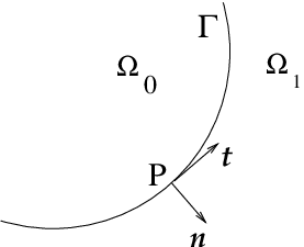
The physical parameters defined in section 2.1 are piecewise constant and can be discontinuous across interfaces. In what follows, we will focus on two domains $\Omega_{0}$ and $\Omega_{1}$, which are separated by a stationary interface $\Gamma$ described by a parametric equation $(x(\tau),\,y(\tau))$ (figure 1). At any point $P$ on $\Gamma$, the unit tangential vector ${\bf t}$ and the unit normal vector ${\bf n}$ are

The derivatives $x^{{}^{\prime}}=\frac{d\,x}{d\,\tau}$ and $y^{{}^{\prime}}=\frac{d\,y}{d\,\tau}$ are assumed to be continuous everywhere along $\Gamma$, and to be differentiable as many times as required.

The evolution equations (6) must be completed by a set of jump conditions. The simple case of perfect bonding and perfect hydraulic contact along $\Gamma$ is considered here, modeled by the jump conditions [18]:

Enforcing these conditions is one of the main objective of the immersed interface method presented in section 3.3.

The eigenvalues of ${\bf A}$ and ${\bf B}$ in (8) are real: $\pm\overline{c}_{pf}$, $\pm\overline{c}_{ps}$, $\pm\overline{c}_{s}$, and 0 (multiplicity 2), where $\overline{c}_{pf}>\max(\overline{c}_{s},\,\overline{c}_{ps})>0$. If $\eta\neq 0$, the spectral radius $R({\bf S})=\frac{\eta}{\kappa}\,\frac{\rho}{\chi}$ can be very large and then the system (8) is stiff.

A plane wave ${\bf d}\,e^{i(\omega\,t-{\bf k}.\,{\bf r})}$ is injected in (6), where ${\bf k}=k\,{\bf e}$ and ${\bf d}$ are the wavevector and the polarization, respectively; ${\bf r}$ is the position, $\omega=2\,\pi\,f$ is the angular frequency and $f$ is the frequency. If ${\bf d}$ is collinear with ${\bf k}$, the dispersion relation of compressional waves is obtained:

where the roots $\pm k_{pf}$ and $\pm k_{ps}$ satisfy $0<\Re\mbox{e}\left\{k_{pf}\right\}<\Re\mbox{e}\left\{k_{ps}\right\}$. If ${\bf d}$ is orthogonal with ${\bf k}$, the dispersion relation of the shear wave is obtained:

where the roots are $\pm k_{s}$, $\Re\mbox{e}\left\{k_{s}\right\}>0$. Based on (13) and (14), the phase velocities $c=\omega/\Re\mbox{e}\left\{k\right\}$ and the attenuations $\alpha=\Im\mbox{m}\left\{k\right\}$ of each wave are defined. In the remainder of this article, the subscripts $pf$, $ps$ and $s$ denote fast compressional, slow compressional and shear waves, respectively.

The phase velocities $c_{pf}(f)$, $c_{ps}(f)$ and $c_{s}(f)$ are monotonically increasing functions, tending asymptotically towards the eigenvalues $\overline{c}_{pf}$, $\overline{c}_{ps}$ and $\overline{c}_{s}$. If $\eta=0$, the three waves are non-dispersive and non-dissipative, and the energy of poroelastic waves (9) is conserved. If $\eta\neq 0$, the fast compressional wave and the shear wave are weakly dispersive and dissipative. The slow compressional wave, however, is highly modified by the viscosity of the saturating fluid. If $f\ll f_{c}$, then $c_{ps}(f)\ll\overline{c}_{ps}$, and the slow compressional wave tends towards a static diffusive mode [10]. At greater frequencies, $c_{ps}$ is larger but the attenuation increases. These properties are summarized in figure 2.

In the low-frequency range, the direct contribution of the slow compressional wave to the overall wave propagation processes is therefore negligible when considering an homogeneous medium. However, the influence of the slow wave becomes crucial in heterogeneous media [6]. The slow compressional wave, generated during the interaction between the propagative waves and the scatterers, remains localized around the interfaces. Consequently, this slow wave has a major influence on the balance equations at the interfaces, modifying crucially the behavior of fast compressional and shear diffracted waves. An accurate computation of the slow wave is therefore necessary, as shown in the numerical tests of section 4.

To integrate the system (8), a uniform grid is introduced; the spatial mesh sizes are $\Delta\,x,\Delta\,y$, and the time step is $\Delta\,t$. A straightforward discretization of (8) by an explicit time scheme leads to the following stability condition:

where $\Theta$ is obtained by a Von-Neumann analysis of stability when ${\bf S}={\bf 0}$. In (15), the bound induced by the spectral radius of ${\bf S}$ can be very restrictive. In sandstone saturated with bitumen, for example, the maximal CFL number is roughly $\overline{c}_{pf}\,\Delta t/\Delta x\approx 10^{-12}\ll\Theta$, which is intractable for computations.

We follow here a more efficient strategy based on second-order Strang’s splitting [23], solving alternatively the hyperbolic system

and then the diffusive system with a source term

The linear system (16) is solved by applying any scheme for hyperbolic systems, giving ${\bf U}_{i,j}^{n+1/2}$. In the numerical experiments performed in section 4, a fourth-order ADER scheme is used [42], which involves a centered stencil of 25 nodes. On Cartesian grids, this scheme amounts to a fourth-order Lax-Wendroff scheme [28]. It is dispersive of order 4 and dissipative of order 6, and its stability limit is $\Theta=1$ [43, 25]. Other single-grid schemes can be used without any restrictions.

Since the physical parameters do not vary with time, the diffusive system (17) is solved exactly. For simplicity, null force density is taken: ${\bf F}={\bf 0}$. In this case, $p$ and ${\bf\sigma}$ are unchanged, whereas the velocities become ($k=1,\,2$)

where $T$ depends on the time step (see section 3.4). The splitting (16)-(17) along with exact integration (18) recovers the optimal condition of stability: $\overline{c}_{pf}\,\Delta\,t/\Delta\,x\leq\Theta$.

Since the matrices ${\bf A}$ and ${\bf B}$ do not commute with ${\bf S}$, the theoretical order of convergence falls from 4 to 2 when the viscosity is non-negligible. Using a fourth-order accurate scheme such as ADER 4 is nevertheless advantageous, compared with a second-order scheme such as Lax-Wendroff: the stability limit is improved, and numerical artifacts (dispersion, attenuation, anisotropy) are greatly reduced.

In [38], the authors notice that the first-order splitting does not lead to a correct representation of the slow mode at low frequencies. Nevertheless, the numerous one-dimensional examples provided in [12] demonstrate that the second-order splitting accurately represents the static mode when a sufficient number of discretization points per wavelength is used. This can be obtained by using a local space-time refinement presented in the following section.

The slow wave has much smaller spatial scales of evolution than the wavelength of the other waves. A very fine grid is therefore required to account for its evolution. Since the use of a fine uniform grid on the whole computational domain is out of reach, grid refinement provides a good alternative. In addition, the slow wave remains localized near the interfaces (section 2.4), and hence grid refinement is necessary only around these places. Lastly, even if the slow wave propagates ($\eta=0$) the property $\overline{c}_{pf}\gg\overline{c}_{ps}$ is usually satisfied: consequently, a fine mesh near the interface is still useful to perform accurate extrapolations, as required by the immersed interface method (section 3.3).

We adopt here a space-time mesh refinement approach based on flux conservation [1, 3], which is more naturally coupled to the flux-conserving scheme developed to solve (16). The refined zones are rectangular Cartesian patches with mesh sizes $\Delta\,x\,/\,q,\Delta\,y\,/\,q$, where the integer $q$ is the refinement factor. To reduce the cpu time and to limit the numerical dispersion on the coarse grid, a local time step $\Delta\,t\,/\,q$ is used [22, 40]. When one time step is done on the coarse grid, $q$ time substeps are done on the refined zone. The extrapolated values required to couple coarse and fine grids are obtained by linear interpolation in space and time on the numerical values at the surrounding nodes [25]. In the case of the Lax-Wendroff scheme applied to the scalar advection equation, the stability of the coupling is proven in [2] whatever $q$.

The additional cost induced by mesh refinement can become prohibitive, both concerning the memory requirements and the computational time, because of the $q$ substeps inside one time step. The value of $q$ must be estimated carefully in terms of the physical parameters. For this purpose, the wavelengths $\lambda_{pf}(f_{0})=c_{pf}(f_{0})/f_{0}$ and $\lambda_{ps}(f_{0})=c_{ps}(f_{0})/f_{0}$ are deduced from the dispersion analysis, where $f_{0}$ is the central frequency of the source. The number of fine grid nodes per wavelength of the slow compressional wave and the number of coarse grid nodes per wavelength of the fast compressional wave must then be roughly equal:

The discretization of the interfaces requires special care. A straightforward stair-step discretization of the interfaces introduces a first-order geometrical error and yields spurious numerical diffractions. In addition, the jump conditions (12) are not enforced numerically if no special treatment is applied. Lastly, the smoothness requirements to solve (16) are not satisfied, decreasing the convergence rate of the ADER scheme.

To remove these drawbacks while maintaining the efficiency of Cartesian grid methods, we adapt an immersed interface method previously developed in acoustics and elastodynamics [35, 26, 27, 25]. At the irregular points where the ADER’s stencil crosses the interface $\Gamma$, the scheme will use modified values of the solution, instead of the usual numerical values. The modified values are extrapolations, based on the local geometry of $\Gamma$ and on $r$ successive derivatives of the jump conditions (12). The parameter $r$ is discussed at the end of this section.

Let us consider a point $M(x_{I},\,y_{J})\in\Omega_{1}$ and its orthogonal projection $P$ onto $\Gamma$ (figure 3). The algorithm to build the modified value at $M$ is divided into four steps.

The numerical strategy presented in this section couples three numerical methods: a finite difference numerical scheme with splitting (section 3.1), a space-time mesh refinement (section 3.2), and an immersed interface method (section 3.3). To clarify the interactions between these methods, the global algorithm is summarized as follows:

Five tests are proposed along this section. In Test 1, the convergence order of the ADER scheme coupled with the immersed interface method is measured. Test 2 illustrates the different kind of waves in homogeneous media, and also the influence of the local space-time refinement. Test 3 investigates the numerical stability of the global algorithm. Diffraction of a plane wave by one (Test 4) and four (Test 5) cylindrical scatterers illustrates the accuracy and the physical relevance of the proposed numerical methods.

The physical parameters given in table 2 correspond to Cold Lake sandstone and shale saturated with water [14], respectively. In some experiments, an inviscid saturating fluid is artificially considered: $\eta=0$ Pa.s, the other parameters being unchanged. As recalled in section 2.1, this limit-case has physical significance only in the high-frequency range. It is mainly addressed here for a numerical purpose.

Once the spatial mesh sizes $\Delta\,x$ and $\Delta\,y$ are chosen on the coarse grid, the time step follows from the CFL number in $\Omega_{0}$: $\overline{c}_{pf0}\,\Delta\,t/\max{(\Delta\,x,\Delta\,y)}=0.95<1$. If $\eta\neq 0$, the maximum CFL number induced by (15) is equal to 0.5: consequently, the simulations done here with the splitting (16)-(17) are twice faster than with unsplitted methods.

The grids are excited by two means: either a plane fast compressional wave, either a point source that generates cylindrical waves. Details of the excitation method are given in C. In the case of an incident plane wave, the exact expression given in C is also enforced numerically on the edges of the computational domain. No special attention is paid to simulate outgoing waves, for instance with Perfectly-Matched Layers [31, 46]. In all the presented tests, the size of the domain and the number of iterations are chosen to avoid the spurious reflections of diffracted waves with the outer frontiers.

In Test 1, we focus on the coupling between the ADER scheme (section 3.1) and the immersed interface method (section 3.3). For this purpose, we consider a domain $[0,\,400]$ m² cut by a plane interface with slope 60 degrees. The saturating fluids are inviscid: exact solutions can be computed very accurately without Fourier synthesis, and splitting errors of the scheme are avoided. The source is plane (41), with parameters: $\gamma=10^{-3}$, $f_{0}=40$ Hz, $t=3.3\,10^{-2}$ s, and $\theta=-30$ degrees (figure 4-a). Consequently, the incident wave propagates normally to the interface, leading to a 1-D configuration; from a numerical point of view, however, the problem is fully bidimensional.

The computations are done on a uniform grid of $N\times N$ points, during $N/4$ time steps. Comparisons with the exact values of the pressure $p$ are done on the subdomain $[50,\,350]\mbox{ m}\times[150,\,250]$ m, in order to avoid spurious effects induced by the edges of the computational domain (figure 4-b). The measures involve reflected and transmitted fast and slow compressional waves generated by the interface (no shear wave is generated in 1D); these waves are highly sensitive to the discretization of the jump conditions.

Errors in $l_{2}$ norm and convergence rates are reported in table 3 and drawn on figure 5. Various values of $r$ are investigated; $r=0$ means that no immersed interface method is applied; in this case, first-order accuracy is obtained. As stated in section 3.3, fourth-order accuracy is maintained if $r=4-1=3$, i.e if third-order extrapolations are used in the immersed interface method. In the present test case, $r=2$ is sufficient to obtain the same level of accuracy on a large range of grid size. Nevertheless, this could be untrue in other contexts, and hence we will always use $r=3$ in the following simulations.

References

- [1] M. J. Berger, J. Oliger, Adaptative mesh refinement for hyperbolic partial differential equations, J. Comput. Phys., 53 (1984), 484-512.
- [2] M. J. Berger, Stability of interfaces with mesh refinement, Math. Comput., 45 (1985), 301-318.
- [3] M. J. Berger, R. J. LeVeque, Adaptive mesh refinement using wave-propagation algorithms for hyperbolic systems, SIAM J. Numer. Anal., 35-6 (1998), 2298-2316.
- [4] M. A. Biot, Theory of propagation of elastic waves in a fluid-saturated porous solid. I: Low-frequency range, J. Acoust. Soc. Am., 28-2 (1956), 168-178.
- [5] M. A. Biot, Theory of propagation of elastic waves in a fluid-saturated porous solid. II: High-frequency range, J. Acoust. Soc. Am., 28-2 (1956), 179-191.
- [6] T. Bourbié, O. Coussy, B. Zinszner, Acoustics of Porous Media, Gulf Publishing Company (1987).
- [7] J. M. Carcione, G. Quiroga-Goode, Some aspects of the physics and numerical modeling of Biot compressional waves, J. Comput. Acoust., 3 (1995), 261-280.
- [8] J. M. Carcione, Wave Fields in Real Media: Wave Propagation in Anisotropic, Anelastic, Porous and Electromagnetic Media, Elsevier (2007).
- [9] J. M. Carcione, C. Morency, J. E. Santos, Computational poroelasticity - a review, Geophysics, 75-5, in press (2010).
- [10] R. N. Chandler, D. L. Johnson, The equivalence of quasi-static flow in fluid-saturated porous media and Biot’s slow wave in the limit of zero frequency, J. Appl. Phys., 52 (1981), 3391-3395.
- [11] M. Chekroun, L. le Marrec, B. Lombard, J. Piraux, O. Abraham, Comparisons between multiple scattering methods and direct numerical simulations for elastic wave propagation in concrete, Springer Proceedings in Physics, 128 (2009), 317-327.
- [12] G. Chiavassa, B. Lombard, J. Piraux, Numerical modeling of 1-D transient poroelastic waves in the low-frequency range, J. Comput. App. Math., 234-6 (2010), 1757-1765.
- [13] O. Coussy, Mechanics of Porous Continua, John Wiley and Sons (1995).
- [14] N. Dai, A. Vafidis, E. R. Kanasewich, Wave propagation in heterogeneous porous media: a velocity-stress, finite-difference method, Geophysics, 60-2 (1995), 327-340.
- [15] B. Dupuy, L. De Barros, J. Virieux, S. Garambois, Wave propagation in heterogeneous porous media formulated in the frequency-space domain, to be published in Geophysics (2011).
- [16] A. Ezziani, Modélisation de la propagation d’ondes dans les milieux viscoélastiques et poroélastiques, PhD thesis, University Paris-Dauphine, (2005).
- [17] S. Feng, D. L. Johnson, High-frequency acoustic properties of a fluid/porous solid interface. I. New surface mode, J. Acoust. Soc. Am., 74 (1983), 906-914.
- [18] B. Gurevich, M. Schoenberg, Interface conditions for Biot’s equations of poroelasticity, J. Acoust. Soc. Am., 105-5 (1999), 2585-2589.
- [19] B. Gustafsson, The convergence rate for difference approximations to mixed initial boundary value problems, Math. Comput., 29-130 (1975), 396-406.
- [20] H. Haddar, J. Li, D. Matignon, Efficient solution of a wave equation with fractional order dissipative terms, J. Comput. App. Math., 234-6 (2010), 2003-2010.
- [21] D. L. Johnson, J. Koeplik, R. Dashen, Theory of dynamic permeability and tortuosity in fluid-saturated porous media, J. Fluid. Mech., 176 (1987), 378-402.
- [22] P. Joly, J. Rodriguez, An error analysis of conservative space-time mesh refinement methods for the one-dimensional wave equation, SIAM J. Numer. Anal., 43-2 (2005), 825-859.
- [23] R. J. LeVeque, Finite Volume Methods for Hyperbolic Problems, Cambridge University Press (2002).
- [24] T. Lin, J. Sochacki, R. Ewing and J. George, Some grid refinement schemes for hyperbolic equations with piecewise constant coefficients, Mathematics of Computation, 56-193 (1991), 61-86.
- [25] B. Lombard, Modélisation Numérique de la Propagation et de la Diffraction d’Ondes Mécaniques, HDR thesis, Aix-Marseille 2 (2010), http://tel.archives-ouvertes.fr/docs/00/44/88/97/PDF/Hdr.pdf.
- [26] B. Lombard, J. Piraux, Numerical treatment of two-dimensional interfaces for acoustic and elastic waves, J. Comput. Phys., 195-1 (2004), 90-116.
- [27] B. Lombard, J. Piraux, Numerical modeling of elastic waves across imperfect contacts, SIAM J. Scient. Comput., 28-1 (2006), 172-205.
- [28] F. Lörcher, C. Munz, Lax-Wendroff-type schemes of arbitrary order in several space dimensions, IMA J. Numer. Anal., (2005), 1-28.
- [29] J. F. Lu, A. Hanyga, Wave field simulation for heterogeneous porous media with singular memory drag force, J. Comput. Phys., 208 (2005), 651-674.
- [30] F. Luppé, J. M. Conoir, S. Robert, Coherent waves in a multiply scattering poro-elastic medium obeying Biot’s theory, Waves in Random and Complex Media, 18-2 (2008), 241-254 .
- [31] R. Martin, D. Komatitsch, A. Ezziani, An unsplit convolutional perfectly matched layer improved at grazing incidence for seismic wave propagation in poroelastic media, Geophysics, 73-4 (2008), 51-61.
- [32] Y. J. Masson, S. R. Pride, K. T. Niheu,Finite-difference modeling of Biot poroelastic equations at seismic frequencies, J. Geophys. Res., 111 (2006), B10305.
- [33] Y. J. Masson, S. R. Pride,Finite-difference modeling of Biot poroelastic equations across all frequencies, Geophysics, 75-2 (2010), 33-41.
- [34] C. Morency, J. Tromp, Spectral-element simulations of wave propagation in porous media, Geophys. J. Int., 175 (2008), 301-345.
- [35] J. Piraux, B. Lombard, A new interface method for hyperbolic problems with discontinuous coefficients: one-dimensional acoustic example, J. Comput. Phys., 168-1 (2001), 227-248.
- [36] T. J. Plona, Observation of a second bulk compressional wave in a porous medium at ultrasonic frequencies, App. Phys. Lett., 36-4 (1980), 259-261.
- [37] W. H. Press, S. A. Teukolskyn, W. T. Vetterling, B. P. Flannery, Numerical Recipes in C: The Art of Scientific Computing, Cambridge University Press (1992).
- [38] J. de la Puente, M. Dumbser, M. Käser, H. Igel, Discontinuous Galerkin methods for wave propagation in poroelastic media, Geophysics, 73-5 (2008), 77-97.
- [39] J. R. Rice, M. P. Cleary, Some basic stress diffusion solutions for fluid-saturated elastic porous media with compressible constituents, Rev. Geophys., 14-2 (1976), 227-241.
- [40] J. Rodriguez, Raffinement de maillage spatio-temporel pour les équations de l’élastodynamique, PhD thesis, University Paris-Dauphine, (2004).
- [41] M. Schanz, Application of 3-D time domain boundary element formulation to wave propagation in poroelastic solids, Eng. Anal. Bound. Elem., 25 (2001), 363-376.
- [42] T. Schwartzkopff, M. Dumbser, C. Munz, Fast high order ADER schemes for linear hyperbolic equations, J. Comput. Phys., 197-2 (2004), 532-539.
- [43] J. C. Strikwerda, Finite Difference Schemes and Partial Differential Equations, Chapman & Hall (1999).
- [44] L. N. Trefethen, Stability of finite-difference models containing two boundaries or interfaces, Math. Comput., 45-172 (1985), 279-300.
- [45] F. Wenzlau, F., T. M. Müller, Finite-difference modeling of wave propagation and diffusion in poroelastic media, Geophysics, 74-4 (2009), 55-66.
- [46] Y. Q. Zeng, J. Q. He, Q. H. Liu, The application of the perfectly matched layer in numerical modeling of wave propagation in poroelastic media, Geophysics 66-4 (2001), 1258-1266.
- [47] C. Zhao, W. Li, J. Wang, An explicit finite element method for Biot dynamic formulation in fluid-saturated porous media and its application to a rigid foundation, J. Sound. Vib., 282 (2005), 1169-1181.