Homodyne estimation of quantum states purity by exploiting covariant uncertainty relation.

Quantum pure states can be faithfully described by their wavefunction $\psi\left(x\right)$. Experimentally producing and measuring pure quantum states is impossible due to the imperfections both of the generation procedures and the measurement apparata. In particular quantum states of the optical fields are always mixed due to impossibility of transmitting and detecting optical fields with 100% efficiencies. Density matrix $\hat{\rho}$ formalism encopasses the possibility of describing both pure and mixed state. In this context an important parameter is represented by the purity $\tilde{\pi}$ given by the trace of the squared density matrix operator with $\tilde{\pi}=1$ for pure states while $\tilde{\pi}<1$ for mixed ones. Moreover, $\tilde{\pi}$ assumes a relevant role in quantum information protocols [1], where the fidelity, i.e. the rate of success, depends critically on the purity of the states. $\tilde{\pi}$ also can give a quantitative measure of the decoherence the pure state have suffered.

Pure states satisfy the Schrödinger [2] and Robertson [3] basic inequalities that generalize Heisenberg [4] uncertainty relations including contributions from covariance of conjugate quantum observables. In Ref. [5] (see also [6]) a new bound, higher than the Schrödinger-Robertson, which accounts for the contribution of the purity of mixed states was found. In Ref. [7] the Schrödinger-Robertson uncertainty relation was expressed in terms of homodyne tomograms. The generic tomographic approach to quantum systems was reviewed in [8]. Combining the purity dependent bound and its expression in terms of homodyne tomograms give rise to a method for a simple determination of the state purity via homodyne detection developed in [9, 10, 11, 12, 13, 14].

The problem of measuring the position and momentum was discussed also in connection with the tomographic approach recently in [15].

So far, evaluation of purity in continuous variable (CV) systems is obtained once the full state density matrix have been reconstructed by quantum tomographic methods. In this paper we prove that the purity of the analyzed state can be retrieved by a very simple and fast analysis of homodyne data thus giving the possibility of having an on-line monitor on the state.

The aim of the present paper is twofold. On the one hand we express the purity $\tilde{\pi}$ of a mixed state in terms of homodyne tomograms, i.e. quantities amenable to an experimental determination. On the other hand, relying on the uncertainty relations of Ref. [5] we derive a simple estimator for the purity of a thermal state which is independent from its tomographic expression.

In Ref. [16] a probability representation of quantum mechanics was suggested in which states are described by standard probability distributions, called tomograms. This representation is based on the representation of the Wigner function $W\left(p,q\right)$ of a quantum state by means of the Radon integral transform or marginal distributions (optical tomograms) [17, 18]. These data representing the output of optical homodyne detectors allows reconstructing the Wigner function using the experimental data. This tomography procedure is nowadays a routine method for measuring quantum states (see for a review [14, 19]). In the present paper, using ideas discussed in [7], we apply the optical tomography to check generalized Schrödinger-Robertson uncertainty relations for conjugate quadratures in the case of a mixed quantum state, in particular, for measuring the effective temperature of a state. The idea of our consideration is based on suggestion [16] (see, also [8]) that the homodyne tomogram is a primary object identified with the quantum state. Due to this, one can extract all information on the state properties including the purity from the measured tomogram only, avoiding the reconstruction of the Wigner function procedure.

The paper is organized as follows.

In section 2, starting from the symplectic forms we give an expression of the purity parameter and of the mean photon number of any mixed photon state in terms of measurable optical tomograms. For thermal states this expression provides the temperature of the field and the mean photon number thus suggesting to check the accuracy of homodyne detection by comparing photon statistics obtained in this way, i.e., from optical tomograms, and in independent photon counting experiment.

In section 3, we review mixed state uncertainty relations to get an estimation of the purity independent of its tomographic expression, by saturating the bound set by the uncertainty relation found in [5]. Hence, measuring optical tomograms of photon states, we can evaluate the purity of the state, and, in the case of thermal states, study the dependence of the quantum bound on the field temperature, thus obtaining a sort of a thermometer for evaluating the temperature. Also, we obtain an estimation for the mean photon number. Finally, in section 4, an experimental comparison, for thermal states, is performed between our estimation and an independent measure of purity of the state, which allows for evaluating the accuracy of our approximate estimation.

A quantum state, either mixed or pure, is described by a density operator $\hat{\rho}$ with purity parameter $\tilde{\pi}$ given by:

According to [16] the state is described by a symplectic tomogram $\mathcal{W}\left(X,\mu,\nu\right),$ where $X,\mu,\nu$ are real parameters, obtained by the Radon transform of the Wigner function $W\left(p,q\right)$ (hereafter,$\mathrm{\ }\hbar=1$):

with $\delta\left(\hat{X}-\mu\hat{Q}-\nu\hat{P}\right)$ standing for

Accordingly the generalized quadrature operator $\hat{X}\left(\mu,\nu\right)$ depends parametrically on $\mu,\nu$ and its moments are given by:

like means and variances, in terms of homodyne quadrature statistics. In particular,

so that

Accordingly, the mixed state is characterized by the quadrature dispersions $\sigma_{QQ},\sigma_{PP},\sigma_{PQ},$ which in turn can be determined by measuring $\sigma_{XX}\left(\mu,\nu\right)$ for particular values of $\mu,\nu.$ In case of optical tomograms, one has $\mu=\cos\theta,\nu=\sin\theta$ so that the optical field state is characterized by the field quadratures relative to $\theta=0,\pi/2$ and $\theta=\pi/4$ :

Analogously the photon number operator $\hat{n}=\hat{a}^{\dagger}\hat{a}=\frac{1}{2}\left(\hat{Q}^{2}+\hat{P}^{2}-1\right)$ is related to the moments

Hence the accuracy of the homodyne detection could be assessed by comparing $\left\langle\hat{n}\right\rangle$ obtained via optical tomograms with that measured by standard photon counting experiments.

The purity $\tilde{\pi}$ of $\hat{\rho}$ is a functional of $\mathcal{W}\left(X,\mu,\nu\right)$ (see, for example, [8])

or equivalently

having replaced $\mathcal{W}\left(X,\mu,\nu\right)$ with the homodyne marginal distribution

which is accessed in homodyne measurements.

For Gaussian photon states $\mathcal{W}\left(X,\mu,\nu\right)$ reduces to:

which inserted (6) into (5) yields the well-known expression:

For a thermal state $\left(\sigma_{QQ}=\sigma_{PP}=\frac{1}{2}\coth\left(\frac{1}{2T}\right)\ ;\ \sigma_{QP}=0\right)$ $\tilde{\pi}$ reduces to

with $T$ measured in $Kelvin\times K_{B}/\hbar\omega$.

The general uncertainty relation for a mixed state reads [5]

with $\tilde{\pi}$ the purity of the state $\hat{\rho}$. The real, continuous and differentiable function $\Phi(\tilde{\pi}),$ such that $\Phi(\tilde{\pi})\geq 1$ in the interval $0<\tilde{\pi}\leq 1$, has the following piecewise analytic expression (extrema of intervals are given by $2(2k+1)/3k(k+1)$, $k=1,2,\ldots$):

Besides, the function $\Phi(\tilde{\pi})$ can be approximated in the whole interval $(0,1)$ within $1\%$ by the interpolating function [5, 6]:

In Fig. (1) we plot the relative difference between $\Phi^{2}(\tilde{\pi})$, the square of the bound function, and $\widetilde{\Phi}^{2}(\tilde{\pi})$ in order to visualize how good is the approximation.

We generalize the inequality (9) to arbitrary local oscillator phases $\theta$, by using the tomographic uncertainty function $F(\theta)$ introduced in [7]:

Then, by using $\widetilde{\Phi}(\tilde{\pi})$ instead of $\Phi(\tilde{\pi})$, the uncertainty relation reads:

in this way, a relation between the tomographic uncertainty function $F\left(\theta\right)$ and the state purity is set.

We recall that $F\left(\theta\right)$ is defined, by means of the variance of the homodyne quadrature $\hat{X}$

as:

We note that for $\theta=0$ one has

So that, $\left.F\left(\theta\right)\right|_{\theta=0}\geq 0$ is exactly the Schrödinger-Robertson inequality. Moreover, comparing the last expression with the thermal state purity given in Eq. (7) it is easy to see that:

The above expression of the uncertainty function $F\left(\theta\right)$ in terms of tomograms was given in [7].

The physical meaning of the function $F\left(\theta\right)$ is the following. For a local oscillator phase $\theta=0$, it is the determinant of the quadrature dispersion matrix, shifted by $-1/4$ as shown in Eq. (16). For a nonzero local oscillator phase $\theta$, the function $F\left(\theta\right)$ corresponds to the determinant of the dispersion matrix of the quadratures, which are measured in a rotated reference frame in the quadrature phase space. The non-negativity of the function $F\left(\theta\right)$ implies the fulfilling of the Schrödinger-Robertson uncertainty relation for all the unitarily equivalent position and momentum operators, since the unitary transformations do not change the canonical commutation relations. The formula (15) simply expresses the determinant of the dispersion matrix for unitarily rotated position and momentum, in terms of tomographic probability distribution $\mathcal{W}_{0}(X,\theta)$.

Thus, the tomogram must satisfy the inequality (12), or (13), where the parameter $\tilde{\pi}$ is expressed in tomographic terms by Eq. (5). However, we can get an estimation of the purity in terms of the tomographic uncertainty function $F\left(\theta\right)$ by saturating the inequality (13). In other words, we consider the minimum value $F$ of the uncertainty function $F\left(\theta\right)$ and estimate that for such a value the inequality is pretty near saturated. Then, by solving with respect to $\tilde{\pi}$, we are able to express the purity as a function of $F$. This is a simple expression:

whose plot is shown in Fig. 2.

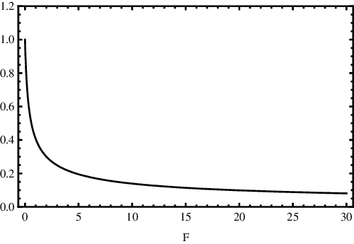
As one can see, $F=0$ corresponds to a pure state, $\tilde{\pi}=1$, and the purity is a smooth decreasing function, going to zero for $F$ at infinity.

On the other hand, for thermal states the purity parameter is directly related to the temperature, i.e. $\tilde{\pi}=\tanh(1/2T)$, so that the previous inequalities and estimations can be translated in terms of temperature. So, in particular, for a thermal state the bound $\tilde{\Phi}$ in inequality (13) can be written in terms of the temperature $T$.

Moreover, $F\left(\theta\right)$ provides the temperature $T\left(F\right)$ of a thermal state with the corresponding purity $\tilde{\pi}\left(F\right)$. We get

We recall that for a thermal state the tomographic uncertainty function $F(\theta)$ does not depend on the local oscillator phase $\theta$, as shown in [7], so that $F(\theta)=F,\ \forall\theta$.

Finally, we remark that for a thermal state the mean value of the photon number can be expressed as a function of the temperature as

so we have a relation between our estimation of the temperature $T\left(F\right)$ and the photon statistics.

In other words, we may check the accuracy of our estimation of the purity and the temperature, resulting from inequality (13), by comparing our estimation of $\left\langle\hat{n}\right\rangle$, i.e.

with an independent measure of the mean number of photons. This comparison is discussed in the next section.

We conclude this section by observing that if the state is not thermal, but we succeed in finding the value $F$ saturating the uncertainty inequality to introduce an effective temperature $T_{eff}.$ This effective temperature is again given by the right hand side of Eq. (18) and corresponds to a purity parameter $\tilde{\pi}\left(F\right)$.

Being the uncertainty relations related to optical tomograms through the tomographic function $F\left(\theta\right)$ (see Eq. (12)) experimental data obtained by optical homodyne detector, suitable for retrieving $F\left(\theta\right)$, allow checking the uncertainty relation (13). Moreover, $F\left(\theta\right)$ allows to evaluate $\tilde{\pi}$, the state purity (Eq. (17)), and in the case of thermal state, $T$, the field temperature (Eq. (18)), and $\left\langle\hat{n}\right\rangle$, the mean photon number (Eq. (20)).

Thermal states are Gaussian so for these states also Eq. (7) is valid. Thus, in order to asses the reliability of the proposed method, it is possible to compare the estimations of $\tilde{\pi}$ via $F\left(\theta\right)$ with the same quantity obtained by using Eq. (7). Moreover, a full reconstruction of the state via quantum tomography provides a further estimation of $\tilde{\pi}$.

To this end, $F\left(\theta\right)$ has been retrieved for thermal continuous wave (CW) states, outing a sub-threshold non-degenerate optical parametric oscillator (OPO) [20]. In such a device non–linear fluorescence gives rise to a pair of down-converted entangled modes each in a thermal state [21]. The experimental setup, illustrated in greater details elsewhere [20, 21], can be sketched into three distinct blocks: the state source, the below threshold OPO, the detector, a quantum homodyne, and the acquisition board.

The quantum homodyne detector, shows an overall quantum efficiency $\eta=0.88\pm 0.02$ (see Refs. [22, 23, 12] for details). The system is set to obtain a $2\pi$–wide linear scanning of the LO phase in an acquisition window. Since $F\left(\theta\right)$ is retrieved by combining variances of data distributions calculated at different $\theta$, we have decided to retrieve $F\left(\theta\right)$ in $[0,\pi]$.

In order to use our homodyne data to calculate $F\left(\theta\right)$, we must be sure that the state is effectively a thermal one. First we prove that the state is Gaussian by performing some tests to assess the Gaussianity of data distribution [24]. In particular, we have used the kurtosis excess (or Fisher’s index) and the Shapiro-Wilk indicator. The kurtosis is a measure of the ”peakedness” of the probability distribution of a real-valued random variable while the Shapiro-Wilk one tests the null hypothesis that a distribution $x_{1},...x_{n}$ came from a normally distributed population. Then, a pattern function tomographic analysis is used for assuring the thermal character of the state [25, 12] and for reconstructing the state Wigner function.

$F\left(\theta\right)$ is calculated by analyzing the data distributions (each distribution containing 2100 data) at $47$ different values of $\theta$ (each $\theta$ value then corresponds to a phase interval interval of $0.067$ rad) and making use of Eq. (15).

A typical output is reported in Fig. 3. The traces are obtained by subtracting to each experimental value of $F\left(\theta\right)$, $\bar{F}_{shot}$ corresponding to the average of $F\left(\theta\right)$ over $\theta$ for a vacuum state whose data are collected by obscuring the homodyne input. $F\left(\theta\right)$ for a shot noise trace returns the $0$ of the instrument. Furthermore, in order to avoid any influence on the statistics of the data, the electronic noise is kept $\approx 15$ dB below the shot noise. The values of $F\left(\theta\right)$, always positive as predicted by the uncertainty relation (13), are with a good approximation independent of $\theta$ as expected for a thermal state.

We have analyzed 218 homodyne acquisitions of thermal states. This large number allows a statistical approach for analyzing the reliability of the proposed method. In particular the purity $\tilde{\pi}$ of the state has been evaluated: a) by reconstructing the state via homodyne tomography ($\tilde{\pi}_{tom}$); b) by using Eq. (17) ($\tilde{\pi}_{F}$); c) by using the exact expression for a thermal state (see Eq. (7)) ($\tilde{\pi}_{th}$).

In Fig. 4 we report the values of the differences $\Delta_{F-tom}$ (a) and $\Delta_{th-tom}$ (b) between $\tilde{\pi}_{F}$ and $\tilde{\pi}_{tom}$ and $\tilde{\pi}_{th}$ and $\tilde{\pi}_{tom}$ normalized to their average. $\tilde{\pi}_{tom}$ has been taken as a reference ¹¹ 1 The tomographic value is the one giving the lower error due the very high statistical reliability of such quantum state reconstruction method.. By looking at these distributions it is seen that while $\Delta_{th-tom}$ is normally distributed (see inset in Fig. 4 (b)) with an average of 0.022 (standard deviation 0.018) $\Delta_{F-tom}$ presents a sistemathic behavior in $\tilde{\pi}$ thus signalling the onset of systemathic error in the obtained determination. While $\tilde{\pi}_{th}$ comes from the exact expression of Eq. (7), $\tilde{\pi}_{F}$ is obtained by approximating $\phi\left(\tilde{\pi}\right)$ (see Eq. (11)) so that the relative precision depends on the purity itself. It has to be noted that in any case the maximum relative error remains below $15\%$.

Comparing $\tilde{\pi}_{F}$ and $\tilde{\pi}_{th}$ evidenziate this effect even better (see Fig. 5).

The above discussed discrepancies, even not so small, confirms that the estimation of $F\left(\theta\right)$, much more simpler than any full state reconstruction methods [14] gives many reliable information on the homodyned state. Moreover, for a thermal state it is possible to obtain more precise information by exploiting Eq. (7).

By exploiting the thermal character of the states herein analysed it is possible to get information on $T$ (Eq. (18)) and $\left\langle\hat{n}\right\rangle$ averaging the experimental trace for $F\left(\theta\right)$ over $\theta$. The values so obtained are given in the following table (together with their confidence interval):

The analyzed mode has $\nu\approx 3\times 10^{14}$ $Hz$ so that the field temperature is of the order $\approx 10^{4}$ $\mathrm{K}$.

Uncertainty relations for mixed quantum states [5, 6] contain information that allows to easily estimate the purity once a connection between optical tomograms and these relations is set. In this paper it is shown that quadrature statistics of the field contains complete information on bound in the generalized uncertainty relations of mixed state and that this bound is intimately related to the state purity. This approach gives the possibility of a fast and reliable estimation of the purity parameter for quantum states that does not require sophysticate data analysis. As far as we know, all the methods for purity estimation rely on the reconstruction of the whole state density matrix while the approach presented in this paper allows to recover the purity simply calculating the tomographic function $F\left(\theta\right)$. The experimental results herein presented show that the homodyne detector can be used as the purity meter of the electromagnetic radiation in the quantum domain. The experimental estimations obtained via $F\left(\theta\right)$ are compatible with more sophysticate estimation obtained via pattern function tomography so proving that our method can be used for real–time evaluations of some basic properties of the homodyne optical states.

Further study of other photon states like squeezed states and multi-mode states will give the possibility to check other quantum phenomena as higher momenta uncertainty relations.

Acknowledgements V.I. Man’ko thanks the University ‘Federico II’ and the Sezione INFN di Napoli for kind hospitality and the Russian Foundation for Basic Research for partial support under Projects No. 09-02-00142.

References

- [1] P. van Lock, Fortschr. Phys. 50, 1177 (2002);
- [2] E. Schrödinger, Ber. Kgl. Akad. Wiss. Berlin, 296 (1930);
- [3] H. P. Robertson, Phys. Rev. 35, 667 (1930);
- [4] W. Heisenberg, Z. Phys. 43, 172 (1927);
- [5] V. V. Dodonov, V. I. Manko, Proceedings of the P.N. Lebedev Physical Institute, Vol. 183 (Nova Science, New York 1989);
- [6] V. V. Dodonov, J. Opt. B: Quantum semiclass. Opt. 4, S98 (2002);
- [7] V. I. Man’ko, G. Marmo, A. Simoni, F. Ventriglia,Adv. Sci. Lett., 2, 517 (2009);
- [8] A Ibort, V I Man’ko, G Marmo, A Simoni, and F Ventriglia, Physica Scripta, 79, 065013 (2009);
- [9] D. T. Smithey, M. Beck, M. G. Raymer, A. Faridani, Phys. Rev. Lett. 70, 1244 (1993);
- [10] J. Mlynek, Phys. Rev. Lett. 77, 2933 (1996);
- [11] A. I. Lvovsky, H Hansen, T. Alchele, O. Benson, J. Mlynek, and S. Schiller, Phys. Rev. Lett. 87, 050402 (2001);
- [12] V. D’Auria, S. Fornaro, A. Porzio, S. Solimeno, S. Olivares, and M. G. A. Paris, Phys. Rev. Lett. 102, 020502 (2009);
- [13] T. Kiesel, W. Vogel, V. Parigi, A. Zavatta and M. Bellini, Phys. Rev. A 78, 021804 (2008);
- [14] A. I. Lvovsky, and M. G. Raymer, Rev. Mod. Phys., 81, 299 (2009);
- [15] J. Kiukas, P. Lahti, J. Schultz, Phys. Rev. A 79, 052119 (2009);
- [16] S. Mancini, V. I. Man’ko and P. Tombesi, Phys. Lett. A 213, 1 (1996);
- [17] J. Bertrand and P. Bertrand, Found. Phys. 17, 397 (1987);
- [18] K. Vogel and H. Risken, Phys. Rev. A 40, 2847 (1989);
- [19] Paris, M., and J. Rĕháẽk, Eds., Quantum State Estimation, Lecture Notes in Physics Vol. 649 Springer, Berlin (2004);
- [20] V.D’Auria, S. Fornaro, A. Porzio, E.A. Sete and S. Solimeno, Appl. Phys. B 91, 309 (2008);
- [21] D. Buono, G. Nocerino, V. D’Auria, A. Porzio, S. Olivares, and M. G. A. Paris, J. Opt. Soc. Am. B, 27:A110 (2010);
- [22] V. D’Auria, A. Chiummo, M. De Laurentis, A. Porzio, S. Solimeno, M. Paris, Opt. Express 13, 948 (2005);
- [23] V. D’Auria, C. de Lisio, A.Porzio, S.Solimeno and M.G.A. Paris, J. Phys. B: At. Mol. Opt. Phys. 39: 1187–1198 (2006);
- [24] J. Řeháček, S. Olivares, D. Mogilevtsev, Z. Hradil, M. G. A. Paris, S. Fornaro, V. D’Auria, A. Porzio, and S. Solimeno, Phys. Rev. A 79, 032111 (2009);
- [25] G. M. D’Ariano, C. Macchiavello and M. G. A. Paris, Phys. Rev. A 50, 4298 (1994).