Internal structure of resonant state in chiral dynamics
Abstract
The internal structure of the resonant state is investigated based on meson-baryon coupled-channels chiral dynamics, by evaluating density distributions obtained from the form factors of the state. The form factors are defined as an extension of the ordinary stable particles and are directly evaluated from the current-coupled meson-baryon scattering amplitude, paying attention to the charge conservation of the probe interactions. For the resonant state we calculate the density distributions in two ways. One is on the pole position of the in the complex energy plane, which evaluates the resonant structure without contamination from nonresonant backgrounds, and another on the real energy axis around the resonance energy, which may be achieved in experiments. Using several probe interactions and channel decomposition, we separate the various contributions to the internal structure of the . As a result, we find that the resonant state is composed of widely spread around , which gives dominant component inside the , with escaping component. Furthermore, we consider bound state without decay channels, with which we can observe the internal structure of the bound state within real numbers. We also study the dependence of the form factors on the binding energy and meson mass. This verifies that the form factor defined through the current-coupled scattering amplitude serves as a natural generalization of the form factor for the resonance state. The relation between the interaction strength and the meson mass shows that the physical kaon mass appears to be within the suitable range to form a molecular bound state with the nucleon through the chiral SU(3) interaction.
Keywords:
, structure; Meson-baryon scattering amplitude; Chiral dynamics; Photon couplings in Bethe-Salpeter equationpacs
13.75.Jz, 14.20-c, 11.30.RdI Introduction
The is a baryonic resonance state with spin-parity , isospin , and strangeness , and is located just below the threshold of antikaon () and nucleon (). This resonance has been considered as a quasi-bound molecule state of the system [1, 2, 3] before the establishment of QCD. In simple constituent quark models, the is classified into the 70 dimensional representation of the spin-flavor SU(6) with excitation of one of the quarks to the -state [4], but it was hard to explain the lighter mass of the than the nucleon resonance in the same representation and the larger spin-orbit splitting between and than the nucleon partners. Recently the was investigated with the unitarized coupled-channels method based on chiral dynamics [5, 6, 7, 8, 9, 10], in which the is dynamically generated in meson-baryon scattering without introducing explicit pole terms. In this method, one can successfully reproduce the cross sections of to various channels together with the mass spectrum of the resonant state below the threshold [5, 6, 7, 8, 11, 12, 13, 14, 15, 16, 17].
One of the important consequences on the structure in the coupled-channels approach is that the is composed of two resonance states [7, 18, 10].11 1 The two-state nature of was pointed out first in Ref. [19] in a different model. These two states have different coupling nature to the meson-baryon states [18, 10], and the state which dominantly couples to the is located at instead of the nominal 1405 MeV. These difference may be important for the system, as the resonance position is measured from the threshold. The double-pole structure also suggests that the resonance position in the invariant-mass spectra depends on the production mechanism of the . Some experimental indications of this structure are found in Refs. [20, 21, 22, 23, 24]. Physical origin of the two poles is attributed to the attractive forces both in the and the channels [25].
Recently, the importance of the meson-baryon dynamical component in the structure of the has been discussed in the chiral unitary framework. It was revealed in an analysis of the phenomenologically obtained scattering amplitude that the is described predominantly by the meson-baryon dynamics [9]. The study of the based on the scaling in chiral unitary framework suggested the dominance of the non- component in the [26, 27]. The electromagnetic mean squared radii were shown to be much larger than that of ground state baryons [28].22 2 The electromagnetic mean squared radii of the was evaluated also in [29] within the framework of the bound-state soliton model. Relationship between the couplings to the channels and the wave function of the was clarified in Ref. [30]. The spatial structure of the was also discussed based on the molecular picture with the chiral potential [31, 32]. The molecular-like structure of the suggests further few-body nuclear systems with kaon [33], such as [33, 34, 35, 36, 37, 38, 39, 31, 32], [40, 41, 42], and [43]. Although the dominant component of the was found to be the meson-baryon molecule structure in these studies, the internal structure of the resonance in terms of the hadronic constituents was not directly extracted from the meson-baryon scattering amplitude.
If the is dominated by the meson-baryon quasi-bound molecule, it may have a spatially larger size, which will lead to the softer form factor than that of typical baryons dominated by the genuine quark component. The soft form factor could result in some experimental consequences, for instance in the nontrivial energy dependence of the photoproduction cross section recently reported in Ref. [44]. The information of the size of hadrons is also important for the production yield in the heavy ion collisions estimated by the coalescence model [45]. One of the standard methods to study the structure of a particle is to use the vector currents, such as the photon, as probes. The properties of the in relation to electromagnetic dynamics have been investigated in the chiral unitary approach in Refs. [46, 47, 48, 18, 49, 50, 51]. In the molecular picture of the , the photon coupling to the is introduced through the photon couplings to its constituent meson and baryon. Among others, the form factor of the will tell us about the intuitive “size” of the particle. Therefore, for both theoretical and experimental understandings of the , it is interesting to investigate the internal structure of the through the evaluation of its form factor.
In this paper we study the form factor of the in chiral unitary approach, in which the is described as the dynamically generated resonance state. We emphasize that this is the first study to extract the form factor of the directly from the scattering amplitude involving the resonance state as a response to the external probe current in a microscopic way. We have already reported the result of the electromagnetic mean squared radii of the in Ref. [28]. Here we extend this scheme to evaluate the momentum dependence of the form factors, using the chiral effective theory of the octet mesons and baryons with the external currents for the elementary interaction between the constituent hadrons and the currents. From the form factors the density distributions can be obtained through the Fourier transformation. This allows us to visualize the spatial distribution of the in coordinate space. We also include the finite size effect of the constituent hadrons.
There is one subtlety in the formulation because the is a hadron resonance and decays via strong interaction. In this case, the form factors (or coupling constants in general) are obtained as complex numbers, whose interpretation is not as straightforward as in the case of the stable particle. Such a difficulty about the complex form factors generally shows up for the unstable states, as seen in the electromagnetic form factors studied in Refs. [52, 53] as complex numbers. Here we carefully define the form factor of the resonance particle as an extension of the ordinary stable particles, and explain the methods to extract the form factors out of the photon-coupled meson-baryon scattering amplitude in a gauge invariant way. In order to achieve the intuitive understanding of the size of the resonance, we evaluate the form factor with several different model set-ups and draw a conclusion through the comparison of the results.
This paper is organized as follows. In Sec. II we explain our scheme to calculate the form factors and the density distributions of the based on the chiral dynamics, taking account of how to extract the information of the “size” of the resonance state. The coupling of the to the external current is obtained by the couplings of its constituent meson and baryon. In Sec. III we show our numerical results of the calculations for the resonant state, on the resonance pole position in the complex energy plane and on the real axis. To obtain the intuitive understanding of the as a quasi-bound state, we consider the bound state without decay width and study its structure by varying the parameters such as the binding energy and the meson mass in Sec. IV. Section V is devoted to the conclusion of this study.
II Formulation
II.1 How to probe structure of resonance state
First of all, we discuss the method to probe the properties of a short-living resonance state. Let us consider an observable represented by a Hermitian operator . One of the simplest and model-independent ways to define resonance properties is given by the evaluation of the matrix element of the operator for the resonance state vectors
| (1) |
This is an extension of the matrix element of the stable particle such as nucleon, . The labels “” and “” represent “in” and “out” states, respectively. Here the ket and bra vectors represent the resonance state in the generalized Hilbert space, whose eigenvalues of the energy-momentum operator are complex as33 3 For the thorough description of the eigenvector for the resonance state, see, e.g., Ref. [54]. See also Ref. [55]. ,
| (2) | ||||
| (3) |
| (4) |
Here and are the mass and decay width of the resonance state, respectively. It is noted that this definition leads to complex values of the matrix elements such as the radius and charge distribution for the resonance state, because the Hermitian operators are allowed to have complex eigenvalues for the resonance state in the generalized Hilbert space. When the decay width of the resonance state is sufficiently small, the imaginary part of the eigenvalues of the Hermitian operators is also small and the matrix elements can be interpreted as physical osbervables in the ordinary sence. In this paper, we mainly discuss the real part of the eigenvalues of the Hermitian operators as “observables”, assuming that the significance of the imaginary part is sufficiently small.
In order to scan the internal structure of the resonance with different probes, we evaluate the matrix elements of various conserved vector currents, the electromagnetic transition current , baryonic current and strangeness current , stemming from the U(1) symmetry of the underlying theory. Electromagnetic current is obtained from the gauged U(1) symmetry with appropriate charges of quarks, baryonic current from the simultaneous U(1) phase transformation for all the quarks, and the strangeness current from the phase rotation for strange quark only. The other currents may also be used as the probes of the structure, as long as the currents are well defined.
The structure of the resonance state is reflected in the form factors, as in the same way with stable particles such as the nucleon. For resonance states with baryon number and spin , we define the form factors as the matrix elements of the probe current ,
| (5) |
where . Especially in the Breit frame the matrix element can be written as [18]:
| (6) |
with the form factors of the time component and the space one , the momentum transfer , , the spinor for the resonance state , and the Pauli matrices for the spin space. For the electromagnetic current, the time component form factor is identified as the electric form factor , whereas the space component form factor as the magnetic form factor . The magnetic form factor is normalized as the nuclear magneton with the proton charge and mass . We define the baryonic form factor and the strangeness form factor as the time component of the matrix elements of the baryonic and strangeness currents, respectively.
The form factors contain the information of the structure of the system in response to the probe interaction, being related to the “classical density” of the system (such as charge density) via the Fourier transformation as,
| (7) |
where is the radial coordinate from the center of mass of the system, and and are the mass and the energy of the state, respectively. Taking the nonrelativistic reduction (), we have,
| (8) |
We can also obtain the mean squared radius:
| (9) |
For the magnetic mean squared radius, we take conventional normalization by dividing the right-hand side of Eq. (9) by the factor . The mean squared radius is well defined when the density sufficiently falls off at large and the integration of converges, which is the case on the poles for the bound states as well as the resonance states.
II.2 Matrix elements of resonance state in scattering amplitudes
Here we explain the method to extract the matrix elements of the resonance state from the scattering amplitudes of dynamical approaches [18, 28]. Once the matrix elements are extracted, following the prescription given in the preceding subsection, we can evaluate the form factors [from Eq. (6)] and density distributions [from Eq. (8)].
 |
 |
| (a) | (b) |
 |
 |
 |
Let us here consider -wave meson-baryon scattering () amplitude with the total energy , in which the excited baryon appears as a resonance state. Performing the analytic continuation of the energy variable to the complex plane , we obtain the scattering amplitude in the complex energy plane. The resonance state is expressed as a pole of the scattering amplitude in the second Riemann sheet. We define the “pole contribution” of the amplitude as
| (10) |
where the pole position is expressed as the resonance mass and width as and the indices and represent the final and initial meson-baryon channels, respectively. The residue at the pole position can be interpreted as the product of the coupling strengths to the meson-baryon channels and . On the real energy axis, the full scattering amplitude can be written as
| (11) |
The contributions which are not represented by the pole term is summarized as a nonresonant background term (see also [56]).
Next we relate the meson-baryon scattering amplitude with the matrix element of the resonance state vectors introduced in the preceding subsection. The pole contribution in the scattering matrix is written as
| (12) | ||||
| (13) |
with
| (14) |
where () is the out (in) -wave meson-baryon scattering state with channel () and momentum (). The total energies are given by and . In this way, the residue of the pole in the scattering amplitude is related to the inner product of the resonance state with the scattering state, representing the coupling strength. It is important that
| (15) |
in Eq. (12) can be understood as the “projection operator” to the resonance state of the mass , which is a generalization of that of the usual stable particle. This resonance component of the amplitude, , is represented diagrammatically in Fig. 1(a).
In the same way, we also consider the scattering amplitude for the process, where stands for a probe such as photon for the electromagnetic current. The Fourier component of the matrix element of the probe current in the -wave meson-baryon state, , is given as:
| (16) |
with incoming and outgoing momenta of the meson-baryon system and , respectively, and . The resonance contribution to the matrix element is obtained by inserting the “projection operator” (15) for the resonance state on both sides of the current operator:
| (17) |
where we have used Eqs. (5) and (14). Hence, the pole contribution to the scattering amplitude of process is
| (18) |
which is represented diagrammatically in Fig. 1(b) (here and following in this subsection we omit the superscript in and ). It is important that this term contains the matrix element of the probe current with the resonance state as the residue of double pole at .
The rest contributions of the amplitude has less singularity at the resonance position . We show several examples of these contributions diagrammatically in Fig. 2, in which the current does not couple to the intermediate resonance propagator.
Combining Eqs. (10) and (18), the matrix elements in the Breit frame can be evaluated as the residue of the single pole at of in the complex energy plane:
| (19) |
As one can see from the above derivation, this scheme indicates that only the amplitude () with the single- (double-) pole terms contributes to the right-hand side, whereas both nonresonant background term in Eq. (11) for and the less singular terms for automatically drop and have no effect to the form factors for the resonance state. As confirmed in Ref. [28], the form factor obtained in Eq. (19) is a gauge invariant quantity.
Equation (19) should be evaluated in the complex energy plane for the resonance state. It is an interesting issue how the matrix elements of the currents for the resonance can be obtained on the real axis, in which amplitudes are in principle observed experimentally. In order to keep closer connection to experimental measurements, we discuss a method to evaluate the form factor of the resonance state on the real axis, as developed in Ref. [18].
As we have seen above, the matrix element of the current for the resonance state is expressed as the residue of the amplitude at the resonance pole position (). If we take the Breit frame of the resonance (), the form factor of the resonance can be written on the real axis as,
| (20) |
where represents less singular terms than the double-pole contribution given in the first term. It is important to note that, if the decay width of the resonance state is small and its pole position is close to the real energy axis, the double-pole amplitudes will give dominant contribution to the process than the other contributions in the resonance energy region.
Motivated by Eq. (20), we define an effective form factor on the real axis as
| (21) |
As discussed in Appendix A, the effective form factor (21) is correctly normalized so as to give the corresponding charge of the system at independently of , if we consider all of the appropriate diagrams giving both the double-pole and less singular terms.
Let us study the relation between the effective form factor (21) on the real axis and the form factor at the pole position (19). Around the resonance energy region, where the pole contribution dominates the amplitude, the derivative of the scattering amplitude (11) with respect to is written as
| (22) |
Assuming that the background contribution is smoothly changing with respect to the energy around the resonance energy and, thus, neglecting the second term of Eq. (22), we can write the effective form factor approximately as
| (23) |
In this way, the effective form factor is related to the resonance form factor . The deviation mainly comes from the less singular terms in which contribute to the effective form factor . Nevertheless, as seen in Eq. (23), if we take the energy close to the resonance mass and choose the channel which strongly couples to the resonance, we can reduce the contamination from the less singular terms. In addition will coincide with evaluated by Eq. (19) when we take by analytic continuation, since in this case both the less singular contribution in Eq. (23) and the nonresonant background contribution in Eq. (22) automatically drop at .
II.3 in chiral dynamics
In this subsection, we briefly review our formulation of the resonance generated dynamically in the process using chiral unitary model (ChUM) developed in Refs. [5, 6, 7, 8]. It turns out that explicit pole terms are not necessary in the elementary interaction for the description of the in ChUM [9].
The starting point of our formulation is the important fact that chiral symmetry and its spontaneous breakdown in QCD constrain the form of low-energy interactions including Nambu-Goldstone bosons. This is systematically expressed in chiral perturbation theory [57, 58, 59], in which the effective Lagrangian is sorted out according to chiral expansion. From the lowest order meson-baryon chiral Lagrangian, the tree-level -wave meson-baryon interaction known as the Weinberg-Tomozawa term can be obtained as,
| (28) |
with the incoming and outgoing meson momenta, and , the meson decay constant , the Clebsch-Gordan coefficient fixed by the group structure of the interaction, and masses of outgoing and incoming baryon, and , respectively. The last form in Eq. (28) is obtained by applying the nonrelativistic reduction for the baryons. The explicit value of the coefficient for the scattering is given in Ref. [6].
Only this lowest-order Weinberg-Tomozawa interaction, however, is not sufficient for the description of the scattering amplitude, especially for three flavors. The main reason is the existence of the baryonic resonance state in and channel, just below the threshold, which spoils any perturbative expansion around the threshold. Therefore, in order to reproduce the scattering amplitude, some nonperturbative and coupled-channels treatment for the scattering is needed.
One valuable approach to take into account the nonperturbative effect is to formulate a scattering amplitude fulfilling exact unitarity with the N/D method [60]. Following Ref. [7], with assumption that the intermediate states of the scattering are composed of only one octet meson and one octet baryon and with neglect of the left-hand cuts, one can write the inverse of the general form of the scattering amplitudes fulfilling unitarity as,
| (29) |
where,
| (30) | ||||
| (31) |
Here denotes the subtraction point, is the threshold value of of the channel and center-of-mass momentum in the channel
| (32) |
where represents the meson mass in the channel .
The function takes the same form as, except for an infinite constant, the ordinary meson-baryon loop integral,
| (33) |
where is an infinitesimal real constant to specify the boundary condition. With dimensional regularization scheme, which keeps analytic properties of the loop function, the finite part of the loop integral can be written as,
| (34) |
with the regularization scale and the subtraction constant .
For the in Eq. (29), we adopt the matching scheme developed in Ref. [7], which tells that the identification of with the tree-level amplitudes by chiral perturbation theory is valid up to . Hence in our approach we identify the Weinberg-Tomozawa interaction in Eq. (28) as . In this way, the -matrix is written in matrix form as,
| (35) |
This amplitude satisfy the following equation
| (36) |
which corresponds to the Bethe-Salpeter equation in algebraic form. We hence refer to this as the BS amplitude. In the present approach we have 10 meson-baryon channels, , , , , , , , , , and .
Now we fix the parameters in our approach; we have the masses of the ground state mesons and baryons, the meson decay constant , and the subtraction constant with the regularization scale . We use the isospin-averaged masses for the mesons and baryons:
For the meson decay constant , we choose an averaged value with , which is one of the typical values used in ChUM. Finally we choose the subtraction constant so as to reproduce the threshold properties of observed in stopped capture on hydrogen [61, 62], as done in Ref. [5],
| (37) |
with the regularization scale [11].
In the present model, the is dynamically generated in the obtained BS scattering amplitude. With above parameters, the model well reproduces the mass spectrum below the threshold [23]. Furthermore, in the present model the is expressed by two poles of the scattering amplitude in complex energy plane, as () and () [10]. The study of the renormalization condition reveals that the resonance in this approach is dominated by the meson-baryon molecule state and the effect from the possible seed of the resonance in the subtraction constant is found to be small [9]. It has been reported in Refs. [17, 25] that the position of the lower pole is largely dependent on details of the model parameters, whereas that of the higher pole shows little dependence.
The residues of the meson-baryon scattering amplitude at the pole position express coupling strengths of the resonance to the meson-baryon channels as seen in Eq. (10). The coupling strengths of the two poles and obtained in the present formulation are listed in Table 1.44 4 The coupling strengths are shown in the particle basis. To compare with the coupling strengths from the amplitude in the isospin basis as in Ref. [10], a factor should be multiplied with the isospin multiplicity for and , and for . From this Table, one can see that the lower pole strongly couples to the state, whereas the higher pole dominantly couples to the state. Among the poles, the higher one is considered to be originated from the bound state [25]. Since we are interested in the structure of the in the bound state picture, we mainly consider the contribution from the higher pole and regard the lower pole as the background.
| Channel | coupling () |
|---|---|
| (, ) | |
| (, , ) | |
| (, ) | |
| Channel | coupling () |
| (, ) | |
| (, , ) | |
| (, ) |
II.4 Electromagnetic interactions in chiral dynamics
As discussed in Sec. II.2, photon-coupling to the resonance state is obtained as the residue of the second-rank pole in the amplitude. This process can be calculated by making a photon couple to the scattering process which has been obtained in the previous subsection to describe the . For the calculation of the process, we take a picture that the photon couples to the resonance state only through its constituent mesons and baryons [18, 28], which may be valid in view of the dominance of the meson-baryon component in the [9]. Thus, we need only electromagnetic interactions of the constituent mesons and baryons in our approach.
Due to the requirement of the gauge invariance, the elementary couplings of the photon to the mesons and baryons should be given by gauging the chiral effective Lagrangian in a consistent way with the description of the . The photon couplings to the meson and baryon appearing in the BS amplitude are derived in the minimal coupling scheme. In addition, the anomalous magnetic couplings in the and vertices are given by the chiral perturbation theory as done in Ref. [18]. The sum of the above two contributions determines the elementary electromagnetic couplings for , for , and for , respectively.
Now let us consider the minimal coupling scheme. The photon coupling to the meson, , is given by
| (38) |
with the meson charge , the incoming and outgoing meson momenta and . The minimal coupling of the photon to the baryon is given by
| (39) |
with the baryon charge and the incoming and outgoing baryon momenta and . These two couplings (38) and (39) are appropriate with the propagators in the loop function (34). For the coupling, we use the following vertex, which is required by the Ward-Takahashi identity at tree-level with the Weinberg-Tomozawa interaction (28):
| (40) |
with the incoming and outgoing meson-baryon total momenta and , respectively, and . We note that this coupling does not contain the magnetic part. Actually for the electromagnetic properties of the neutral excited baryon this term does not contribute due to . This is a different point compared with Ref. [18], where the normal magnetic part coming from the original form of the Weinberg-Tomozawa term (II.3), proportional to , was introduced.
For the anomalous and couplings which are gauge invariant by themselves, we use the interaction Lagrangian appearing in the chiral perturbation theory [63]:
| (41) |
with
| (42) |
the electromagnetic field tensor , the charge matrix , the spin matrix , the SU(3) matrix of the baryon octet field , and the chiral field where is the SU(3) matrix of the Nambu-Goldstone boson field. This interaction Lagrangian gives us spatial components of both the and the vertices ():
| (43) | ||||
| (44) |
where we have made nonrelativistic reduction. Here the anomalous magnetic moment for the baryon and the matrix are given by,
| (45) |
| (46) |
where the coefficients , , , and are fixed by the flavor SU(3) symmetry and their explicit values are found in Ref. [18]. The values of the coefficients and are determined to be and so as to reproduce the observed anomalous magnetic moments of the baryons55 5 Here we note that in Ref. [18] the additional contribution () was introduced in order to take into account the normal magnetic part of the gauged Weinberg-Tomozawa interaction. This is unnecessary in our calculation, where , because Eq. (40) does not produce the magnetic part. . In the calculation, these values are used for the vertices (44), while for the baryon anomalous magnetic moments we use the experimental values instead of (45). For the unobserved magnetic moment, we use the SU(3) flavor relation , which is consistent with quark models. The transition magnetic coupling does not contribute in the isospin symmetric limit, because this interaction changes the isospin of the excited baryon to . Now the total coupling and the vertex are given by the sum of the normal and anomalous contributions:
| (47) | ||||
| (48) |
where is the observed magnetic moment of the baryon.
Here we note that the magnetic interactions of the excited baryons are obtained only from the baryonic dynamics, since in our approach the spinless meson is bound by the baryon in -wave channel and the spatial component of the couplings do not contribute to the magnetic interactions in the Breit frame of the excited baryons.
In order to study the internal structure of the theoretically, we also consider the form factors probed with the baryonic and strangeness currents. For the baryonic and strangeness current interactions, we replace the meson and baryon electric charges with the corresponding quantum numbers, namely, the baryon number and strangeness of the mesons and baryons:
| (49) |
for the baryonic current and
| (50) | ||||
for the strangeness current. Then we consider the time components as the form factors for the baryonic and strangeness current interactions, as described below Eq. (6). Since the baryonic and strangeness form factors are calculated by the time component of the current, we do not need the counterparts of the matrices and given in Eq. (46), which contribute to the spatial component.
II.5 Calculation of photon-coupled meson-baryon amplitudes
 |
 |
 |
 |
 |
 |
 |
 |
 |
 |
Now we discuss the details of the calculation of the scattering amplitude of the process in the chiral unitary approach, in which the amplitude for the is given by multiple scattering of the meson and baryon.
One of the most important issues we take account of is the charge conservation in the calculation of the scattering amplitude for the process. This ensures the correct normalization of the form factor of the excited baryon, , , and . Following the method proposed in Refs. [48, 64, 28], to calculate the form factors we take three relevant diagrams shown in Fig. 3, which contain the double-pole terms for the resonance states. Although charge conservation requires seven other diagrams as shown in Fig. 4 for the general amplitude [64], these diagrams cannot contribute to the matrix elements at the resonance pole calculated by Eq. (19), since these terms have at most a single pole [28]. This means that, on the resonance pole, the charge conservation is maintained by only three diagrams shown in Fig. 3. Summing up the diagrams in Fig. 3, we obtain the relevant amplitude for the evaluation of the form factors:
| (51) |
These contributions can be expressed by the combination of the BS amplitude and the elementary couplings discussed before, according to the Feynman diagrams given in Fig. 3. In the Breit frame, in which the momenta of the photon and the before photon coupling are expressed as and , respectively, their explicit forms are written as:
| (52) | ||||
| (53) | ||||
| (54) |
where the vertex is given in Eq. (48) and the loop integrals with the photon couplings to the meson and baryon are given by,
| (55) | ||||
| (56) |
In the Breit frame and , and , , and are functions of and . The function () at is related to the loop integral given in (34) as,
| (57) |
| (58) |
which can be easily proved by calculating the derivative of the loop integral and using the vertices (38) and (47). Other analytic properties of these loop integrals, and , are discussed in Appendix B. 66 6 If one adopts the cut-off procedure for the meson-baryon loop integral , one must calculate the photon-coupled meson-baryon loop integrals and in a consistent way with the same cut-off. Form factors of in such a cut-off procedure were evaluated in Ref. [30]. The two approaches, the dimensional regularization in our procudure and the cut-off procedure, would not make much differences in form factors except for the high momentum region compared to the cut-off scale.
Now we introduce the finite size effects of the constituent hadrons in our scheme. The ground state mesons and baryons have spatial structures, while we have implicitly assumed that they are pointlike particles in the effective Lagrangian approach. Therefore we should include the finite size effects of the constituent hadrons in a gauge invariant way. Here we simply multiply a common form factor (CFF) of the constituent hadrons to each photon vertex,
| (59) | ||||
| (60) | ||||
| (61) |
Note that the only depends on so it can be factorized out from the loop integrals of Eqs. (55) and (56). In this study we employ the dipole type form factor as,
| (62) |
We take , which reproduces nucleon form factors well. This CFF corresponds to the hadron density with radial coordinate of each hadron and mean squared radius .
Here we comment on the normalization of the effective form factor obtained on the real axis. As discussed in Appendix A, the effective form factor is correctly normalized so as to give the corresponding charge of the system at independently of the energy , if we consider all of the diagrams shown in Figs. 3 and 4. Among them, the three double-pole diagrams in Fig. 3 give dominant contributions at the energies close to the resonance pole position. Therefore, even if we take into account only the three diagrams in Eq. (51), deviation from the correct normalization for the effective form factor is considered to be small. We also note that a part of the less singular terms in (hence ) is included in these three diagrams because off the pole position the nonresonant background in [see Eq. (11)] generates less singular parts in Eqs. (52)–(54). Here we choose the channel for the evaluation of for the , which reduces the contribution from the less singular terms thanks to the large coupling strength , as demonstrated in Eq. (23).
At last, let us show a relation among electric (), baryonic (), and strangeness () form factors for the based on isospin symmetry, in which we have a generalized Gell-Mann-Nishijima relation for the probe current,
| (63) |
with the current for the third component of the isospin, . Taking the matrix element for the with , we obtain77 7 At , we obtain the usual Gell-Mann-Nishijima relation, , for hadrons,
| (64) |
where the matrix element of vanishes for the state. From the relation (64), we have the relation for the spatial densities,
| (65) |
with radial coordinate as well.
III Numerical Results
In this section, we discuss the internal structure of the resonant state. We will show the numerical results of the form factors measured by the electromagnetic, baryon number, and strangeness currents in momentum space. We will also show the spatial density distributions in coordinate space which are obtained by performing Fourier transformation of the form factors.
The calculation of the form factor is performed in two ways; one is on the pole position (Sec. III.1 and the other is to evaluate the effective form factor (21) on the real energy axis around the resonance energy region (Sec. III.2. On the pole position, the internal structure of the resonance can be obtained in a way to keep charge conservation without nonresonant background contributions. The results, however, may not be directly compared with experimental observables. The effective form factor on the real energy axis, on the other hand, may be determined in experiments, but the obtained form factors have both the resonant and nonresonant contributions.
For a reference of the electric size of the typical neutral baryon, we will compare the electric form factor with an experimental fit of neutron electric form factor [65],
| (66) |
with , , , the neutron mass , and the neutron magnetic moment , where is the nuclear magneton.
We also compare the results of magnetic, baryonic and strangeness form factors with a dipole type form factor,
| (67) |
with , which reproduces well the observed nucleon magnetic form factor [66]. The overall factor will be adjusted to the normalization of the form factor of the in question.
III.1 Form factors on the resonance pole
Here we discuss the internal structure of the using the form factors obtained at the pole position in the complex energy plane. We evaluate the form factors of the higher state, , out of two states, since this state gives the dominant contribution to the spectrum and is considered to be originated from the bound state. The form factors of the at the resonance position are obtained by Eq. (19) together with the amplitudes calculated in Eqs. (36) and (51).
III.1.1 Electromagnetic, baryonic, and strangeness structures
 |
 |
First of all, we show our results of the electric and magnetic form factors in Fig. 5 together with the empirical form factors of the neutron given in Eqs. (66) and (67). The normalization parameter is given by the real part of the magnetic moment of the , . Here, in order to see the finite size effects of the constituent hadrons, we also show results without the common form factor (CFF) introduced in Eq. (62). The finite size effects make the magnitude of the form factors reduced, especially in the large region. Hereafter, we show only the results with CFF unless explicit mentionings.
Now let us discuss the electromagnetic form factors of the resonant shown in Fig. 5. The form factors and contain the imaginary parts, since they are evaluated on the resonance pole position in the complex energy plane. However, we obtain the imaginary parts in smaller magnitude than the real parts. This is the consequence of the relatively small imaginary part of the pole position of , since the form factors are real numbers in the limit of zero imaginary part of the pole position. For the charge neutral , deviation from zero in the electric form factor indicates that the has a nontrivial charge distribution as seen in the neutron form factor. Comparing the real part of the form factor and the empirical neutron form factor, we find that the form factor has larger magnitude than that of the neutron, especially at low . This indicates that the spatial structure of the is larger than the neutron. For the magnetic form factor of the , to which only the baryon components contribute as seen in Sec. II.4, the real part of the result shows faster decreasing than the dipole fit to the nucleon. These results of and suggest the peculiar electromagnetic structure of the compared with the typical neutral baryon such as the neutron.
 |
Next we discuss the baryonic and strangeness form factors of the using the baryonic and strangeness currents as external probes. The calculation is done in the same way as the electric form factor using the baryonic charge (49) and the strangeness charge (50) instead of the electric charge. The baryonic and strangeness form factors, and , are plotted in Fig. 6. For comparison, the strangeness form factor is presented with the opposite sign. Because of the baryon number and strangeness conservation in our formulation the form factors are correctly normalized as and , respectively. From Fig. 6 we find that the imaginary parts of the total baryonic and strangeness form factors are small compared with their real parts, as in the case of the electromagnetic form factors. We can also see that both the baryonic and strangeness form factors give steeper derivative at compared with the nucleon form factor, and that the strangeness form factor shows faster decreasing than the baryonic one. Hence, the baryonic and strangeness components also imply the peculiar structure of the resonant among the ordinary low-lying hadrons.
 |
 |
Now it is interesting to visualize the spatial structure of the resonant in coordinate space as the density distributions and the mean squared radii obtained from the form factors using Eqs. (8) and (9). We introduce a normalized density distribution with the density distribution . With this definition, integrating from to , one gets the total charge (or magnetic moment) of the system:
| (68) |
In Fig. 7 we plot the electromagnetic density distributions of the . As we can see from the left panel, the real part of the charge distribution has large magnitude compared with that of the neutron. This may indicate smaller overlap between positively and negatively charged components in the than in the neutron. It is also found that the charge distribution has positive values in the inner part ( fm) and negative values in the outer part ( fm). Since the () strongly couples to the channel, the charge form factor of the is expected to be dominated by the component. Hence, our result implies that the lighter surrounds the heavier . From the magnetic distribution (Fig. 7, right) we can see the spatially larger structure of the compared with the neutron. Since the magnetic density distribution is contributed mainly from the magnetic moment of the baryon in the , the magnetic structure reflects the baryonic component.
 |
In the same way, the baryonic and strangeness density distributions are plotted in Fig. 8 with the typical density distribution of the nucleon, which is evaluated by the Fourier transformation of the dipole form factor in Eq. (67) with . For comparison, the strangeness density distribution is shown with the opposite sign. The baryonic and strangeness density distributions clearly indicate the dominance of the real parts over the imaginary parts and spatially larger structure than the nucleon. In addition, the strangeness density distribution has a longer tail than the baryonic one. Since the at pole position is dominated by the component, this means larger distributions compared with inside the .
Finally we evaluate the electromagnetic, baryonic, and strangeness mean squared radii, which are calculated using Eq. (9) with the form factor. For the magnetic mean squared radius, we use the calculated magnetic moment as the normalization of the mean squared radius. The results are shown in Table 2. We find that the absolute value of the electric (magnetic) mean squared radius is (), which is about two times larger than that of the neutron (). Also the absolute values of the baryonic and strangeness mean squared radii are larger than the typical size of nucleon. We also observe in Table 2 larger radius of the strangeness distribution than the baryonic one. This is due to the effect of the longer tail in strangeness density distribution compared with the baryonic one. Therefore, these results support that the resonant state has a spatially-extended structure compared with the typical baryon size .
As a consequence, all of the results for the electromagnetic, baryonic, and strangeness structures show that the resonant has a large size compared with typical hadrons. Furthermore, it is interesting to observe that the strangeness density distribution of the has longer tail than the baryonic one. Since the () is dominated by the component and () carries the strangeness (baryon number), one can expect that such behaviors of the strangeness and baryonic distributions are understood by the widely spread distribution around inside the . This expectation is supported by the charge distribution, since it has positive values in the inner part whereas negative values in the outer part, which will be caused by the component inside the . In the next subsection, we will clarify these detailed structure of the by decomposing the form factors and density distributions into the contribution from each meson-baryon component.
III.1.2 Contribution from each meson-baryon component
 |
 |
 |
In order to discuss the inner structure of the resonance from the theoretical point of view, it is interesting to decompose the form factors into the contribution from each meson-baryon state to which the external current couples. This decomposition can be done by calculating the amplitude in Eqs. (52) and (53) without the summation of the intermediate channel , so that the total form factor is obtained by summing up all the components. In the decomposition we do not include the contribution from , which is not important for the study of the spatial size of the resonance, since this is a contact interaction and gives an almost trivial momentum dependence from the form factor of the constituent hadrons88 8 For the electric current, gives no contributions in case of neutral resonances. . Here we mainly discuss the and components in the form factors, since the and intermediate states are the dominant contributions in the resonance as we have seen in Table 1, and we will check that the and channels and the contact term coming from give negligibly small contributions to the form factors.
We first discuss the contributions to the electromagnetic form factors from the and intermediate states. In the upper panel of Fig. 9, we show the electric form factor coming from the and states. As one can see from the figure, the electric form factor from the state reproduces almost the total form factor given in Fig. 5. The reason is as follows; the neutral hadrons do not contribute to the electric form factor, and the resonance () has a tiny coupling to the channel. Then, the sum of the contributions from and components dominate the electric form factor. However, since we are working in the isospin symmetric limit, the states give exactly same contributions in magnitude for the isospin resonance with the opposite sign due to their electric charges. Thus, the sum of the states does not contribute to the total electric form factor for the resonance and the state reproduces almost the total electric form factor.
In the contribution, we observe the sudden increase of the real part and the peak structure of the imaginary part seen at , which comes from the analytic properties of the loop function in which the external current attaches to the pion propagator. We will discuss the details in next subsection and Appendix B.
The separated contributions to the magnetic form factor are shown in the middle and lower panels of Fig. 9. For the magnetic contribution, the meson pole term shown in Fig. 3 does not contribute and we are left with the baryon pole term (and the contact term , which contribution is not included in Fig. 9. Here we show the form factors with the , , and intermediate channels. We find that the contribution is substantially larger than . Here we also find that the contribution has the opposite sign to the and they largely cancel each other. This is because only the isosinglet component can couple to the due to the isospin symmetry and the isosinglet magnetic moment of nucleon is known to be very small. This result indicates that the magnetic form factor of the is composed mainly by nucleons in dynamics in which, however, large cancellation between and components takes place.
| Component | |
|---|---|
| total | |
| Contact |
Next we discuss the contributions to the baryonic and strangeness form factors from each meson-baryon channel. Here, instead of plotting the form factors with respect to , we show in Table 3 the values of the baryonic and strangeness form factors at with individual contributions from the meson-baryon channels to the , which corresponds to the each channel contribution to the baryon number and strangeness of the system. Here we have the Gell-Mann-Nishijima relation at for each meson-baryon channel. The decomposition to each meson-baryon channel implies that the channel gives more than of the total baryonic and strangeness charges, whereas the , , , and contact-term components in channel are negligibly small. The magnitude of the charge of each component is determined by the coupling strength given in Table 1 and the derivative of the loop function which contributes to the form factor through Eqs. (57) and (58). Thus, due to the large coupling strength the channel dominates the structure of the .
 |
 |
 |
Now we show the meson-baryon components of the electromagnetic density distributions, and , which are obtained by the Fourier transformation of the corresponding meson-baryon components of the form factors. The results are shown in Fig. 10. Note that is plotted up to instead of . We find again the dominance of the component in both and . Hence, the negative (positive) charge distribution of the in Fig. 7 is now understood as the lighter (heavier ) existence in outside (inside) region. It is a more interesting finding that the (equivalently with the opposite sign) component of the electric density distribution shows a characteristic behavior of dumping oscillation. As we will discuss in next subsection and Appendix B, the oscillating behavior can be interpreted as the decay of the system into the channels through the photon coupling to the intermediate meson. Although this oscillation is interesting from the theoretical point of view, it does not contribute to the total density distribution due to the cancellation of and components. For the magnetic density distribution, we again observe large cancellation between and components in the isosinglet .
 |
Then, we decompose the baryonic and strangeness density distributions into the different meson-baryon contributions in Fig. 11. In this figure, represents the sum of the contributions from and , whereas represents the sum of the contributions from , , and . For the channel, we plot the baryonic density which is equivalent to the strangeness density with the opposite sign. This is clear from the charges in Eqs. (49) and (50) where both baryonic and strangeness currents probe the component with the same strength and the opposite sign in the intermediate state. As one can see from the Fig. 11, the component where the baryonic (strangeness) current probes the () distribution dominates both the baryonic and strangeness density distribution in Fig. 8. Therefore, the longer tail of the strangeness distribution in Fig. 8 is now understood as the larger distribution of the component than that of the baryon number distribution generated by the . This is consistent with the electric density distribution, that the lighter locates outside the , which should also be the case for the and through the isospin symmetry.
From the decomposition of the form factors and density distributions into meson-baryon components, it is confirmed that the resonant is indeed dominated by the component, giving more than of the total baryonic and strangeness charges, and it is found that the is dominantly composed of the in the outside region around the nucleon, with a large size compared with typical hadrons. We also find that the magnetic moment of the is composed mainly by nucleons in dynamics in which large cancellation between and components takes place. In addition, we observe that the component has the escaping oscillation in the charge distribution (see also next subsection), which is although not observed in the total charge due to the cancellation. In our results all of the results for the electromagnetic, baryonic, and strangeness structure of the are consistent with each other.
III.1.3 Escaping oscillation in decay channel
In the previous subsection we found an interesting behavior of the escaping oscillation in the electric density distribution. Here we discuss the escaping oscillation found in the channel, or decay channel in general.
From a viewpoint of the Fourier transformation, what makes oscillation behavior in the electric density distribution is the peak structure at in the electric form factor in the channel. Namely, the Fourier transformation of the form factor picks up much contributions from the peak structure, making large magnitude in the corresponding wave number for the density distribution, which is seen as the oscillation component.
Then, let us discuss the origin of the peak structure in the form factor. An important point is that the photon coupled loop integral of the intermediate channel , (), contains a divergent point at
| (69) |
with real energy , defined in Eq. (32), and the baryon (meson) mass () in the intermediate state. This divergence point corresponds to the -channel threshold. The detailed discussion is given in Appendix B. It should be emphasized that this singularity (69) can be reached only in case that the energy is above the threshold of the channel, , so that . Such a singularity at certain generates peak structure in the form factor with complex energy through the analytic continuation . Hence, that the resonance energy is above the threshold is essential to the peak structure in the form factors, and the oscillation behavior of the density distributions can be interpeted as the decay of the system into the open channels through the photon coupling to the intermediate state, with kicked meson and baryon to the on-shell by the photon coupling. In the present case, since only the channel is open for the decay, the peak structure appears only in the channel.
From the above discussion, it is obvious that the peak structures in the form factors and the oscillation behaviors in the density distributions should appear in decay channels for resonance states in the meson-baryon picture. Such structures are, however, eventually not observed in the total electric form factor and density distribution for the resonant . This is because, as we have mentioned, the components largely cancel each other for the electric structure due to the isospin symmetry. Hence, if we would observe a excited state for which its decaying channel contributes to the form factors without cancellation, we could observe the escaping oscillation in the total density distribution.
At last, we comment on that the magnetic, baryonic, and strangeness density distributions do not show the (visible) oscillation behavior even in the decay channel, . This is because the magnetic, baryonic, and strangeness currents couple to rather than pion in the channel; the current coupling to the propagator also provides the oscillation behavior in the electric as well as the magnetic, baryonic, and strangeness density distributions. However, Eq. (69) indicates that, due to the small pion mass , the -current coupling makes the peak structure in the form factor with very high value [ for the channel in the ()], thus such a high coupling should be strongly suppressed by form factors of the constituent hadrons. As a consequence, the oscillation contributions from the -current coupling are numerically small and not visible in Figs. 10 and 11.
III.2 Effective form factors on the real energy axis
Now we evaluate the effective form factors of the on the real energy axis defined in Eq. (21), in order to study how the form factors obtained at the resonance position are seen on the real energy axis. These effective form factors on the real axis will provide the quantities which can be compared with the experimental observations, in contrast to the form factors obtained in the complex energy plane. Here we comment that the mean squared radii are not well defined for resonances on the real energy axis due to insufficient fall-off of the densities at large , in contract to the case on the resonance pole position.
 |
As discussed in Sec. II.5, the form factors calculated with three diagrams shown in Fig. 3 keep correct normalizations only on the resonance pole position. Off the resonance pole position the additional diagrams shown in Fig. 4 are necessary to keep the correct normalizations. Nevertheless, since the double-pole diagrams dominate the photon-coupled amplitude at the resonance energies if the pole position is not far from the real axis, the contributions from the supplemental diagrams in Fig. 4 to the form factors may be negligible.
This can be checked by the calculation of the effective baryon number for the state with the diagrams in Fig. 3 on the real axis. Here we choose the channel in with the baryonic current, so that the less singular contributions are suppressed through the large coupling constant [see Eq. (23)]. In Fig. 12, we plot for the on the real energy axis as a function of , which is evaluated with the three diagrams shown in Fig. 3. If the amplitude maintains the conservation law by taking account of all the diagrams, should be pure real and unity independently of . Figure 12 indicates that the real part of calculated with the three diagrams is close to one in the energy . This means that the three diagrams dominate the amplitude of the process, and that contributions coming from the neglected diagrams are less than . To study the energy dependence, we evaluate the form factors at three meson-baryon center-of-mass energies , , and .
 |
 |
The results of the real part of the effective electromagnetic form factors on the real energy axis are shown in Fig. 13. We find that the effective electromagnetic form factors for are qualitatively very similar with the form factors evaluated at the pole position in Fig. 5. We also find in Fig. 13 that the effective electromagnetic form factors have mild energy dependence even in energies close to the resonance position. This is because, off the resonance pole position, less singular terms also contribute to the effective form factors and brings energy dependence to them. We also see that, in the energies closer to the threshold, both the and have steeper change at low .
 |
 |
Now let us discuss the electromagnetic density distributions and obtained from and . We plot the real parts of and in Fig. 14 with , , and , in comparison with the empirical neutron density distribution. The important point is that the effective distribution in the real axis also catches the properties found in the density distribution on the pole position, that is, spatially larger structure than the neutron with the outward negative charge of and the inward positive charge of . As the energy increases, the observed distribution becomes effectively wider.
Finally we summarize the numerical analyses of the internal structure of the resonant state, which is done by evaluating two observables; one is the resonance form factor (19) on the resonance pole position (see Sec. III.1, and the other is the effective form factor (21) on the real energy axis (Sec. III.2. Although there is a quantitative difference between these two analyses such as the energy dependence of the effective form factors, it is found that the several peculiar features of the resonance form factor in the complex plane are mostly maintained in the effective form factor on the real axis. This means that the properties of the defined in the complex plane may be within our reach of the experimental searches achieved by the real energies. This consequence comes from the small imaginary part of the pole of the .
From these analyses we have drawn the following conclusions. The has softer form factors than those of neutron. Consequently the mean squared radii are larger than the neutron radii which can be regarded as a typical baryon, as found in Ref. [28]. Through the decomposition into meson-baryon channels and the analysis of the form factors with different probe currents, the internal structure of the resonant is found to be dominated by the component, with the nucleon in the center being surrounded by the antikaon.
IV Discussions
We have considered the form factors and density distributions of the resonant state. Because the resonance has the finite decay width, the obtained form factors are complex numbers. Although we have deduced the structure of the mainly from the behavior of the real part of the form factors, the interpretation may not be as straightforward as the stable particle.
The has been considered as a quasi-bound state of the system99 9 In this section represents channel in the isospin basis. having the decay channel [1, 2]. This picture is also supported by the chiral unitary approach, where the bound state is generated only by the attractive interaction and channel coupling to provides the with the decay width [25]. In the present study, we confirmed this picture by the decomposition of the baryonic charge in the previous section. Therefore, it is instructive to understand the structure of the bound state, by switching off the couplings of to other channels.
In the case of the bound sate, the form factors are obtained as the real numbers for all , hence we can interpret the form factors as physical quantities. Furthermore, the single-channel model allows us to investigate the internal structure of a dynamically generated bound state. For instance, we expect that the spatial size will be larger for the system with smaller binding energy. This does not trivially follow from the calculation of the form factor and is worth examining in the present framework. Thus, we examine the structure of the bound state by changing the model parameters.
In Sec. IV.1, we will study the structure of the bound state with the natural subtraction constant , which is obtained so as to exclude explicit pole contributions from the loop function [9]. This ensures that the bound state has the pure molecule structure. Then we will study the structure of the dynamically generated bound states with different binding energies in Sec. IV.2. The interaction strength is adjusted to fix the binding energy within the natural condition. We also discuss the meson-nucleon bound state with different meson masses instead of the physical kaon mass, in order to see the effect of meson masses to the bound state in Sec. IV.3, where the spatial size of the bound state is kept fixed.
IV.1 Structure of the bound state
In this subsection, we consider the single channel model with a bound state. We use the Weinberg-Tomozawa interaction (28) for the channel and the subtraction constant with the regularization scale , which is obtained by the condition [9]. With this subtraction constant, solving the single-channel scattering equation (36) we obtain the bound state at with the coupling strength to the [see Eq. (10)] as . This bound state is generated only by the attractive interaction and has a binding energy of .
 |
 |
Here we first study the structures of the and components in the bound state. Since the () has strangeness () and baryon number (), we can observe and distributions in the bound state by using the strangeness probe current with the opposite sign and the baryonic current, respectively, which leads to the relations for the form factors as,
| (70) |
where represents the () form factors probing the () component in the bound state. We also study the electric structure of the bound state, which is related to the and form factors via the generalized Gell-Mann-Nishijima relation (64). Here we do not consider magnetic component of the bound state. In Fig. 15, the , , and electric form factors are shown together with the empirical form factors of the neutron (66) and (67). Comparing with the previous results for the resonant , we find that all of the electric, , and form factors of the bound state show similar characteristic behaviors with the real part of the electric, baryonic, and opposite-sign-strangeness form factors of the resonant , respectively. For the and form factors , we observe the steeper derivative at compared with the dipole form factor and the faster decreasing form factor than the one, which reflect a salient structure of the bound state, as the resonant discussed before. Also the electric form factor exhibits large enhancement at smaller region () and slowly decrease above , as the real part of the form factor of the resonant .
 |
 |
Using the form factors we calculate the density distributions through the Fourier transformation. In Fig. 16, the , , and charge density distributions from the form factors are shown with the normalization . As we can see from the figure, the behaviors of the density distributions are similar to those for the resonant in Figs. 7 and 8, thanks to the large coupling of the ; the charge distribution has positive values in the inner part whereas the negative values in the outer part, and the distribution has longer tail than the one.
| [fm2] | [fm2] | [fm2] | [fm2] |
|---|---|---|---|
The results of the , , and electric mean squared radii evaluated from the form factors are displayed in Table 4. The results of the and mean squared radii, and , respectively, indicate that both the and distributions spread compared with the typical nucleon size in the bound state, and the has larger distribution than the inside the bound state. The electric mean squared radius is , whose absolute value is four times larger than that of the neutron . Indeed, the charge density distribution clearly shows the larger structure of the bound state than the typical neutral hadron.
Next, it is also interesting to evaluate the mean squared distance between and from the form factors in our approach. For this purpose we take the nonrelativistic limit and treat the constituent hadrons as point particles, neglecting the common form factor effects [see Eq. (62)]. In the nonrelativistic limit, both the and form factors and are determined from the form factor for the relative motion in the two-body system with appropriate scale transformations as,
| (71) |
| (72) |
due to the kinematics of the system. Therefore, the mean squared distance between and , , can be determined from both the and form factors and with appropriate coefficients. The results are given by,
| (73) |
| (74) |
for the mean squared distance between and . The two values in Eqs. (73) and (74) show very good agreement with each other. A small difference between two values in Eqs. (73) and (74) is expected to come from the field theoretical evaluation of the form factor and the relativistic correction with respect to the binding energy. In this study we define the mean squared distance as the average of the values evaluated from the and radii, and we obtain the mean squared distance between and as
| (75) |
for the bound state with binding energy .
IV.2 system with different binding energies
Here we discuss the bound state with different binding energies, in order to see the dependence of the structure on the binding energy. This can be achieved by replacing the interaction strength for in Eq. (28) with representing an interaction strength for to generate a bound state with a specified binding energy , and we keep the subtraction constant in order to exclude the explicit pole contribution. In Fig. 17 we plot interaction strength as a function of the binding energy .


We dynamically generate a bound system with different binding energies and show the electric, , and mean squared radii as functions of the binding energy in Fig. 18. It is obvious that the distribution of the constituent hadrons in the bound state spreads if the binding energy decreases, in accordance with our expectation from quantum mechanics. In addition, the mean squared radii are much sensitive to the binding energy in the near-threshold region (), which indicates that for the shallow bound state the binding energy is a key quantity for the spatial structure of the bound state. We also find that the distribution in the bound system is more sensitive to the binding energy in this region, since the is lighter than the . In the large binding energy region, the and mean squared radii asymptotically goes to finite values. This behavior in the large binding energy region is caused by that the distributions of both and shrink to the finite and radii. In contrast, the electric radius goes to zero, because and get close to each other, which leads to almost zero electric mean squared radius.

Next let us make a simple comparison of our results of mean squared radii, which is based on the field theory, with that of the nonrelativistic wave function of the two-body bound state, in order to check the consistency of these methods. Outside the interaction range the nonrelativistic wave function for the bound state takes an asymptotic form in the relative coordinate with the distance and the reduced mass . Here we adopt a simple form having the correct asymptotic behavior,
| (76) |
as a typical wave function for comparison. Using this wave function , one can evaluate the mean squared distance of the two particles in the bound state as,
| (77) |
Although it is derived from the specific wave function (76), this relation holds model-independently for the state with small binding energy, where the inner part () of the wave function is irrelevant and the asymptotic form of the wave function dominates the integration in Eq. (77). Now in Fig. 19 we compare our result of the mean squared distance between and , , which is evaluated by using method developed in the previous subsection for a bound state of point particles, with that obtained from the nonrelativistic wave function (77), . As we can see from the figure, the difference between and is quite small for every binding energy. This is an interesting result, because it is nontrivial that the mean squared distance between and in our approach, where the bound state is dynamically generated and the size is probed by external currents within the framework of the field theory, shows very similar value to that from the nonrelativistic wave function .
IV.3 Meson-nucleon bound system with various meson masses
In this subsection, we vary the meson mass from the physical kaon mass, in order to see the effect of the meson mass to the meson-nucleon bound state. Here we consider the meson (, ) having same quantum numbers as the antikaon (, ) except for the mass.
During the calculation, we fix the spatial structure of the bound system so that the meson-nucleon distance is to be in hadronic interaction range. For this purpose, we impose the condition,
| (78) |
where is the binding energy of the system and is the reduced mass, 1010 10 For the study of the different meson masses, we denote the meson mass by . . The interaction strenght is adjusted by the binding energy through (78) and the natural subtraction constant determined by [9]. We start with the bound state with the physical kaon mass which leads as studied in section IV.1. In Fig. 20 we plot interaction strength as a function of the meson mass.


For the meson-nucleon bound state, the electric probe is useful to study the structure of the system, since the electric current probes the negatively charged and positively charged in the bound state, hence we can observe relative distribution of the meson and nucleon in the system as well as the spatial size of the system. In Fig. 21, we show the charge density distribution of the meson-nucleon bound state for different meson masses. As we have discussed for the bound state, in the meson-nucleon bound state, concentration of positive (negative) charge density corresponds to the region dominated by the (). For the small meson mass region (, ), the meson distributes at larger distance than the , as the bound state in the preceding subsections. If the meson mass is compatible with the nucleon mass () the charge distribution is almost flat around zero, which indicates that meson and have almost same distribution, and cancel each other in the charge distribution. For the meson mass larger than the nucleon (, ), the meson and distributions interchange their role, where the lighter nucleon goes outside and the heavier meson stays inside. Such a behavior is consistent with our expectation from the classical picture and indicates that we correctly observe internal structure of the bound state with respect to the mass ratio of the constituent hadrons.
Here we note that the difference of the structures between the bound states of and heavy meson-nucleon, if existed, might be realized as a difference of the behaviors of the bound states in nuclear medium. For the (heavy meson-nucleon) bound state, has smaller (larger) density distribution in the system, which implies that has larger (smaller) momentum distribution due to the uncertainty principle. Therefore, in nuclear medium, where the momentum of is filled up to the Fermi momentum, the existence of heavy meson-nucleon bound state might be suppressed even in the lower density compared with .

It is also illustrative to plot the various mean squared radii and the mean squared distance between meson and nucleon as functions of the meson mass (Fig. 22. The mean squared distance is almost independent of the meson mass, as a consequence of the fixed . This suggests that the spatial size of the bound state is indeed constrained by this condition. The suppression of the mean squared distance in the smaller meson mass region () is caused by the condition that the binding energy, which is restricted by Eq. (78), is not negligible compared with the meson mass. In addition, the electric, mesonic, and nucleon mean squared radii behave consistently with our interpretation discussed above. The sign change of the electric radius at reflects the inversion of the spatial distribution of the meson and .
At last we comment on the relation between the meson mass and the interaction strength . The result in Fig. 20 shows that in the small meson mass region a strongly attractive interaction is required to keep the light meson binding with the nucleon, whereas the heavier meson can be bound as the molecular type (with ) by the moderate attraction, in accordance with the classical expectation. From the group theoretical point of view, the coupling strength of the scattering of the octet baryon and the octet meson is at most [67, 68]. The result in Fig. 20 suggests that if the meson were as light as MeV, we would need the coupling strength to generate a bound state with the size . This means that the pion is too light to generate a bound state of the molecular type1111 11 It is possible to generate a resonance, such as the meson in scattering, the lower pole of the resonance in scattering, and the meson in scattering.. On the other hand, the sufficiently heavy meson mass () is essential to generate a meson-nucleon bound state with spatial size of a hadronic molecular state by using the chiral interaction.
V Conclusion
We have studied the internal structure of the resonant state with electromagnetic, baryonic, and strangeness probes. The resonant state has been described by the meson-baryon interaction picture based on chiral dynamics. The form factors and the density distributions of the have been defined carefully as an extension of ordinary stable particles and been directly evaluated from the meson-baryon scattering amplitude, paying attention to the gauge invariance of the probe interaction.
The internal structure of the resonant with full coupled-channels has been studied in two ways, one on the resonance pole position in the complex energy plane and the other on the real energy axis around the resonance region. The first method has produced the resonant structure as the matrix element of the probe current by the resonance vector without contamination from nonresonant background, and exactly kept the gauge invariance. The second one, on the other hand, has given values which may be observed in experiments while the nonresonant contamination has been involved. We have found that the resonant state has softer form factors and larger spatial radii than those of the typical baryon, and the structure is largely dominated by the component. The charge distribution has indicated that the light distributes around the proton which sits in the central region. The characteristic structure of the shown in the resonance form factor on the resonance pole position can be kept in the effective form factor on the real axis. We have also found that the decay of the into the channel through the photon coupling causes an escaping oscillation pattern in the density distribution in the coordinate space.
We have also discussed internal structure of a bound state without the decay width to extract an intuitive picture of the bound state. We have found the similar structure with the resonant , thanks to the dominance of the component. We also have observed that such a structure shrinks (stretches) as the binding energy increases (decreases), which is consistent with the behavior of the bound state in the quantum mechanics. We have seen the meson mass dependence of the bound state which indicates that the behavior of the relative distribution of the meson and nucleon inside the bound state is consistent with the kinematics of meson-nucleon system. These results have verified that the form factor defined through the scattering amplitude serves as a natural generalization of the form factor for the resonance state. Also the relation between the coupling strength and the meson mass shows that the physical kaon mass appears to be within the suitable range to form a molecular bound state with the nucleon through the chiral SU(3) interaction.
Acknowledgements.
We acknowledge Y. Kanada-En’yo, T. Myo, A. Hosaka, A. Ohnishi, H. Suganuma, and K. Yazaki for useful discussions. This work is partly supported by the Grand-in-Aid for Scientific Research from MEXT and JSPS (Nos. 21840026, 22105507, 22740161, and 22-3389), and the Grant-in-Aid for the Global COE Program “The Next Generation of Physics, Spun from Universality and Emergence” from MEXT of Japan. One of the authors, T.S. acknowledges the support by the Grand-in-Aid for JSPS fellows. T.H. thanks the support from the Global Center of Excellence Program by MEXT, Japan through the Nanoscience and Quantum Physics Project of the Tokyo Institute of Technology. This work is part of the Yukawa International Program for Quark-Hadron Sciences (YIPQS).Appendix A Normalization of form factors
In this Appendix we discuss the normalization of the amplitude induced by a conserved current in the soft limit , where and are the meson-baryon center-of-mass energy and the squared momentum transfer with opposite sign, respectively. Because we are considering the matrix element with the conserved current , the amplitude should automatically be normalized by Ward-Takahashi identity:
| (79) |
where is the amplitude, the “charge” of the meson-baryon system with respect to the probe current, and the indices and stand for the final and initial meson-baryon channels, respectively1212 12 The Ward identity of the general unitarized amplitude was discussed in Ref. [64]. Here we confirm the Ward-Takahashi identity in a derivative form (79) within our formulation. . Thus, we prove that the amplitudes discussed in sections II.3 and II.4 satisfy Eq. (79), concentrating on the case.
In this study the meson-baryon amplitude is obtained as the solution of the Bethe-Salpeter (BS) equation
| (80) |
with the interaction kernel and the meson-baryon loop integral [see Eq. (36)]. The amplitude is obtained by evaluating ten diagrams given in Figs. 3 and 4 in which the probe current is attached to the meson-baryon scattering amplitude. Among them, the amplitudes , , , and diverges in the soft limit . These terms correspond to the infrared divergences coming from the bremsstrahlung processes of the external hadrons and are canceled by the vertex corrections, leaving no contributions to the amplitude at . Hence, in the soft limit, only the six diagrams are relevant for ,
| (81) |
with each contribution calculated in our formulation as,
| (82) |
| (83) |
| (84) |
| (85) |
| (86) |
| (87) |
where the loop integrals with photon couplings , , and the vertex function are defined in Sec. II.
The key relations for proving Eq. (79) are the derivative of the vertex and the loop integrals at ,
| (88) |
| (89) |
Equations (88) and (89) are the Ward-Takahashi identity for the elementary vertex and two-body free propagator . Thus, if the vertex and the loop integrals and conserve the charge associated with the current, Eqs. (88) and (89) should be satisfied. Then, using these relations and the BS equation (80), we can prove Eq. (79) by an algebraic calculation. Omitting the superscript and evaluating all the terms at , we can write the left-hand side of Eq. (79) as,
| (90) |
where we have use Eqs. (80) and (88). From Eqs. (85) and (86), the first and second terms in the right-hand side of (90) are and , respectively. Replacing in the third term of Eq. (90) with , we have,
| (91) |
From Eqs. (82) and (83) with (89), the second term of the right-hand side in (91) is equal to . Then, using the product rule of the differentiation for the third and fifth terms of Eq. (91), we have,
| (92) |
From Eqs.(84) and (88), the second term in the parenthesis in Eq. (92) is . Therefore, collecting remained terms,
| (93) |
Then, using Eqs. (80), (87), and (88), we finaly achieve from the left-hand side of Eq. (79) to its right-hand side,
| (94) |
Thus, with (81), we obtain Eq. (79). We note that this relation is valid at any value of the meson-baryon center-of-mass energy , even in complex energy plane. Since Eq. (79) is the relation between meson-baryon scattering amplitude and that with photon attached, the existence of the resonance pole is not necessary for the argument above.
The relation (79) immediately leads to correct normalization of the effective form factor defined in Eq. (21), as,
| (95) |
This normalization is achieved at any energies , regardless of existence of the resonance, as long as one includes all the relevant contributions in Eq. (81). If there exists the resonance pole at the complex energy in the meson-baryon scattering, taking limit we see that coincides with the resonance form factor evaluated in Eq. (19). Hence the relation (79) also guarantees the correct normalization of the resonance form factor . In the case that the energy is close to the resonance pole position ( in our case) on the real axis, the charge will be dominated by the contributions from the three diagrams in Fig. 3, as discussed in Sec. II.5.
We also derive, from Ward-Takahashi identity (79), a relation between the coupling strengths of the resonance state to the meson-baryon channel and the derivative of the vertex and the loop function :
| (96) |
To prove Eq. (96), we consider explicit forms of and for the resonance contribution. The derivative of the amplitude is shown in Eq. (22). The amplitude has double-pole terms for the resonance as well as the less singular terms. The former corresponds to Fig. 3 and is expressed in Eqs. (82)–(84), while the latter does to Fig. 4 and is in Eqs. (85)–(87). Using the explicit form of given in Eq. (11) and the Ward-Takahashi identity (88) and (89) for the double-pole terms, can be expressed as,
| (97) |
where represents the less singular terms than the double-pole contribution. Thus, calculating and taking limit , both the nonresonant contribution in and less singular terms in automatically drop and we have,
| (98) |
hence, we obtain Eq. (96). This is the exact form of the relation between the coupling strength and the derivative of the loop integral , discussed in [69, 30]. Equation (96) exactly corresponds to the relation known as the Ward identity:
| (99) |
with the vertex-renormalization factor and the wave-function one , respectively. In our case with the resonance state, is the residue of the resonance contribution in the meson-baryon scattering amplitude, , and is the current-coupling term,
| (100) |
through Eqs. (88) and (89). Using and , Eq. (96) can be rewritten as,
| (101) |
Appendix B Loop integrals and
In this Appendix we discuss the properties of the loop integral [given in Eqs. (55) and (56)], which describes that one photon is attached to the one of the internal propagators. For concreteness, we consider the electromagnetic probe interaction for the .
 |
 |
 |
 |
Integrating over the four-momentum in Eqs. (55) and (56) in the Breit frame for the , these functions are explicitly written with the Feynman parameters and as
| (102) |
| (103) |
| (104) |
| (105) |
Here , , and are the charge of the meson and baryon, and magnetic moment of the baryon in channel, respectively, and is defined in Eq. (32) so that is simply written as,
| (106) |
with the Källen function . We note that spatial components of the loop integrals in which photon couples to mesons vanish in the Breit frame, , since the pseudoscalar mesons do not have the magnetic moments. In the above equations the integrations are analytically performed; the integrations can in principle be done analytically, but we perform the numerical integration in the practical calculation with keeping to be a small finite value, which ensures the correct boundary condition during the analytic continuation.
As one can see from Eqs. (102)–(105), the integrands in are obtained in the analytic form for the energy and the squared photon momentum , hence we can make an analytic continuation from the real to the complex value, , for the integrands.
In our study we perform the analytic continuation of in a following way. At first, we fix and make a complex value, (: real) so that is continuous with respect to . In this condition, we are in a first (second) Riemann sheet with respect to with () if the energy is above the meson-baryon threshold. Then, we make vary from to finite real values so that are continuous with respect to .
In order to visualize this, we plot the sum of the loop integrals , which appears in the amplitude as in Eqs. (51)–(53), in the - plane. In Fig. 23 we show time component in and channels with the real part of the energy being fixed as , around the pole position of the . Here we note that in all meson-baryon channels for total charge-zero system, the functions vanish at at any complex energies , because at the relations (57) and (58) lead to .
Now we discuss the behavior of the loop integral. One notice that with real-valued energy, that is, . This is interpreted as the fact that and cannot go on-shell simultaneously with the energy below the threshold, . With the real-valued energy (), the real part decreases as we increase . This property of decreasing is visible until around in the analytic continuation to imaginary energy, . For the channel, is smooth in the - plane.
The channel of the loop integral, on the other hand, has some nontrivial behaviors. One is the divergence of the loop integral at finite with real , which is clearly seen in the imaginary part , and another is the discontinuity in the real part running above the same . The divergences of and take place, as will be discussed later, at
| (107) |
respectively. Hence, the loop integral with diverges only when the real-valued energy is above the two-body threshold, so that . Furthermore, this divergence point corresponds to the -channel threshold; with fixed above the threshold, all the three propagating particles can simultaneously go on-shell in () for (), while for () two propagating mesons (baryons) cannot simultaneously go on-shell in () if we constrain the baryon (meson) to go on-shell.
The origin of the divergences of and is the factor in the integrands of Eqs. (102)–(104), where represents the meson mass (the baryon mass ) when the photon couples to the baryon (meson) propagator. By dropping the irrelevant factors, which do not cancel singularity from , and performing the integration, we obtain,
| (108) |
which contains the logarithmic divergence at . Therefore, the loop integral () logarithmically diverges at () with .
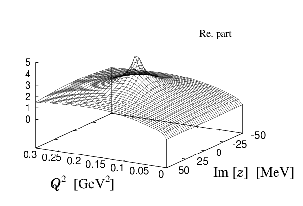 |
 |
Now it is instructive to investigate the behavior of with respect to and . In Fig. 24 we plot as a function of and with conditions and . Here analytic continuation is performed in the same way as for and . From Fig. 24 we can see the real part of contains divergence point at and , whereas the imaginary part of shows discontinuity along the real energy axis above the same value (). These properties are explained by using analytic properties of a logarithm function . Namely, taking limit from any complex energy and any real , we have,
| (109) |
with argument of , , which is finite, hence the divergence appears only in the real part of . Further, in order to see the behavior of the imaginary part of , we first fix the energy with an infinitesimal imaginary part as (). Then, from the divergence point of is fixed as with the square root of the Källen function . Now let us consider with the energy and momentum , where is finite positive value. Since the Källen function gives a relation,
| (110) |
where is an infinitesimal positive value determined by the and and has a property , the numerator and denominator inside the logarithm in Eq. (108) become:
| (111) | ||||
| (112) |
respectively. Therefore, has the limit,
| (113) |
hence the discontinuity appears in the imaginary part of .
As a consequence of the factor in the integrands, , and in the channels with energy above the threshold contains divergence in the imaginary part at and the discontinuity in the real part along the real energy axis above the same value. Here we note that the function (105) is pure imaginary so that the discontinuity (divergence) of the imaginary (real) part of is manifested in the real (imaginary) part of the loop integrals .
 |
 |
These diverging structures in the loop functions eventually lead to the divergences of the effective form factors (21) at , and to the peak structures of the form factors (19) around that . Then, the “peaks” of the (effective) form factors in the momentum space lead to the oscillation components in the density distributions in the coordinate space with period given by through the Fourier transformation. Therefore, for the channel whose threshold is lower than the total energy , we will have an oscillation component of the “decaying part”, which can be interpreted as the decay of the system into the open channels with kicked meson and baryon to the on-shell through the photon coupling.
Here let us show the behaviors of and components of effective form factor and density distribution in electric probe with energy fixed as . The form factor and density distribution on the resonance pole position are shown in Sec. III.1. As you can see, the effective electric form factor in channel shows divergence at , which generates an oscillation behavior in the effective electric density distribution with the period close to .
Finally we note that the oscillation part will be clearly seen only in the case that the probe current couples to the mesons. In this case corresponds to the baryon mass , hence the value appears around typical hadronic scale , which will be important for the dynamics of the hadrons. This is not the case when the probe current couples to baryons, since in this case the value becomes much larger than , due to the light meson masses , especially for pions, , and such a high coupling should be strongly suppressed by form factors of constituent hadrons.
References
- [1] R. H. Dalitz and S. F. Tuan, Annals Phys. 10, 307 (1960).
- [2] R. H. Dalitz, T. C. Wong and G. Rajasekaran, Phys. Rev. 153, 1617 (1967).
- [3] H. W. Wyld, Phys. Rev. 155, 1649 (1967).
- [4] N. Isgur and G. Karl, Phys. Rev. D 18, 4187 (1978).
- [5] N. Kaiser, P. B. Siegel and W. Weise, Nucl. Phys. A 594, 325 (1995) [arXiv:nucl-th/9505043].
- [6] E. Oset and A. Ramos, Nucl. Phys. A 635, 99 (1998) [arXiv:nucl-th/9711022].
- [7] J. A. Oller and U. G. Meissner, Phys. Lett. B 500, 263 (2001) [arXiv:hep-ph/0011146].
- [8] M. F. M. Lutz and E. E. Kolomeitsev, Nucl. Phys. A 700, 193 (2002) [arXiv:nucl-th/0105042].
- [9] T. Hyodo, D. Jido and A. Hosaka, Phys. Rev. C 78, 025203 (2008) [arXiv:0803.2550 [nucl-th]].
- [10] D. Jido, J. A. Oller, E. Oset, A. Ramos and U. G. Meissner, Nucl. Phys. A 725, 181 (2003) [arXiv:nucl-th/0303062].
- [11] E. Oset, A. Ramos and C. Bennhold, Phys. Lett. B 527, 99 (2002) [Erratum-ibid. B 530, 260 (2002)] [arXiv:nucl-th/0109006].
- [12] D. Jido, E. Oset and A. Ramos, Phys. Rev. C 66, 055203 (2002) [arXiv:nucl-th/0208010].
- [13] T. Hyodo, S. I. Nam, D. Jido and A. Hosaka, Phys. Rev. C 68, 018201 (2003) [arXiv:nucl-th/0212026].
- [14] T. Hyodo, S. i. Nam, D. Jido and A. Hosaka, Prog. Theor. Phys. 112, 73 (2004) [arXiv:nucl-th/0305011].
- [15] C. Garcia-Recio, J. Nieves, E. Ruiz Arriola and M. J. Vicente Vacas, Phys. Rev. D 67, 076009 (2003) [arXiv:hep-ph/0210311].
- [16] B. Borasoy, R. Nissler and W. Weise, Phys. Rev. Lett. 94, 213401 (2005) [arXiv:hep-ph/0410305].
- [17] B. Borasoy, R. Nissler and W. Weise, Eur. Phys. J. A 25, 79 (2005) [arXiv:hep-ph/0505239].
- [18] D. Jido, A. Hosaka, J. C. Nacher, E. Oset and A. Ramos, Phys. Rev. C 66, 025203 (2002) [arXiv:hep-ph/0203248].
- [19] P. J. . Fink, G. He, R. H. Landau and J. W. Schnick, Phys. Rev. C 41, 2720 (1990).
- [20] T. Hyodo, A. Hosaka, E. Oset, A. Ramos and M. J. Vicente Vacas, Phys. Rev. C 68, 065203 (2003) [arXiv:nucl-th/0307005].
- [21] S. Prakhov et al. [Crystall Ball Collaboration], Phys. Rev. C 70, 034605 (2004).
- [22] V. K. Magas, E. Oset and A. Ramos, Phys. Rev. Lett. 95, 052301 (2005) [arXiv:hep-ph/0503043].
- [23] D. Jido, E. Oset and T. Sekihara, Eur. Phys. J. A 42, 257 (2009) [arXiv:0904.3410 [nucl-th]].
- [24] D. Jido, E. Oset and T. Sekihara, arXiv:1008.4423 [nucl-th].
- [25] T. Hyodo and W. Weise, Phys. Rev. C 77, 035204 (2008) [arXiv:0712.1613 [nucl-th]].
- [26] T. Hyodo, D. Jido and L. Roca, Phys. Rev. D 77, 056010 (2008) [arXiv:0712.3347 [hep-ph]].
- [27] L. Roca, T. Hyodo and D. Jido, Nucl. Phys. A 809, 65 (2008) [arXiv:0804.1210 [hep-ph]].
- [28] T. Sekihara, T. Hyodo and D. Jido, Phys. Lett. B 669, 133 (2008) [arXiv:0803.4068 [nucl-th]].
- [29] C. L. Schat, N. N. Scoccola and C. Gobbi, Nucl. Phys. A 585, 627 (1995) [arXiv:hep-ph/9408360].
- [30] J. Yamagata-Sekihara, J. Nieves and E. Oset, Phys. Rev. D 83, 014003 (2011) [arXiv:1007.3923 [hep-ph]].
- [31] A. Dote, T. Hyodo and W. Weise, Nucl. Phys. A 804, 197 (2008) [arXiv:0802.0238 [nucl-th]].
- [32] A. Dote, T. Hyodo and W. Weise, Phys. Rev. C 79, 014003 (2009) [arXiv:0806.4917 [nucl-th]].
- [33] Y. Akaishi and T. Yamazaki, Phys. Rev. C 65, 044005 (2002).
- [34] T. Yamazaki and Y. Akaishi, Phys. Rev. C 76, 045201 (2007) [arXiv:0709.0630 [nucl-th]].
- [35] N. V. Shevchenko, A. Gal and J. Mares, Phys. Rev. Lett. 98, 082301 (2007) [arXiv:nucl-th/0610022].
- [36] N. V. Shevchenko, A. Gal, J. Mares and J. Revai, Phys. Rev. C 76, 044004 (2007) [arXiv:0706.4393 [nucl-th]].
- [37] Y. Ikeda and T. Sato, Phys. Rev. C 76, 035203 (2007) [arXiv:0704.1978 [nucl-th]].
- [38] Y. Ikeda and T. Sato, Phys. Rev. C 79, 035201 (2009) [arXiv:0809.1285 [nucl-th]].
- [39] Y. Ikeda, H. Kamano and T. Sato, Prog. Theor. Phys. 124, 533 (2010) [arXiv:1004.4877 [nucl-th]].
- [40] D. Jido and Y. Kanada-En’yo, Phys. Rev. C 78, 035203 (2008) [arXiv:0806.3601 [nucl-th]].
- [41] A. Martinez Torres, K. P. Khemchandani and E. Oset, Phys. Rev. C 79, 065207 (2009) [arXiv:0812.2235 [nucl-th]].
- [42] A. Martinez Torres and D. Jido, Phys. Rev. C 82, 038202 (2010) [arXiv:1008.0457 [nucl-th]].
- [43] Y. Kanada-En’yo and D. Jido, Phys. Rev. C 78, 025212 (2008) [arXiv:0804.3124 [nucl-th]].
- [44] M. Niiyama et al., Phys. Rev. C 78, 035202 (2008) [arXiv:0805.4051 [hep-ex]].
- [45] S. Cho et al. [ExHIC Collaboration], arXiv:1011.0852 [nucl-th].
- [46] N. Kaiser, T. Waas and W. Weise, Nucl. Phys. A 612, 297 (1997) [arXiv:hep-ph/9607459].
- [47] J. C. Nacher, E. Oset, H. Toki and A. Ramos, Phys. Lett. B 455, 55 (1999) [arXiv:nucl-th/9812055].
- [48] J. C. Nacher, E. Oset, H. Toki and A. Ramos, Phys. Lett. B 461, 299 (1999) [arXiv:nucl-th/9902071].
- [49] T. Hyodo, A. Hosaka, M. J. Vicente Vacas and E. Oset, Phys. Lett. B 593, 75 (2004) [arXiv:nucl-th/0401051].
- [50] L. S. Geng, E. Oset and M. Doring, Eur. Phys. J. A 32, 201 (2007) [arXiv:hep-ph/0702093].
- [51] M. Doring, D. Jido and E. Oset, Eur. Phys. J. A 45, 319 (2010) [arXiv:1002.3688 [nucl-th]].
- [52] L. Heller, S. Kumano, J. C. Martinez and E. J. Moniz, Phys. Rev. C 35, 718 (1987).
- [53] S. Kumano, Phys. Lett. B 214, 132 (1988).
- [54] A. Bohm, J. Math. Phys. 22, 2813 (1981).
- [55] A. Bohm, Quantum Mechanics: Foundations and Applications, 3rd ed. (Springer, 2001).
- [56] M. Doring, C. Hanhart, F. Huang, S. Krewald and U. G. Meissner, Phys. Lett. B 681, 26 (2009) [arXiv:0903.1781 [nucl-th]].
- [57] S. Weinberg, Physica A 96, 327 (1979).
- [58] J. Gasser and H. Leutwyler, Nucl. Phys. B 250, 465 (1985).
- [59] A. Pich, Rept. Prog. Phys. 58, 563 (1995) [arXiv:hep-ph/9502366].
- [60] G. F. Chew and S. Mandelstam, Phys. Rev. 119, 467 (1960).
- [61] D. N. Tovee et al., Nucl. Phys. B 33, 493 (1971).
- [62] R. J. Nowak et al., Nucl. Phys. B 139, 61 (1978).
- [63] U. G. Meissner and S. Steininger, Nucl. Phys. B 499, 349 (1997) [arXiv:hep-ph/9701260].
- [64] B. Borasoy, P. C. Bruns, U. G. Meissner and R. Nissler, Phys. Rev. C 72, 065201 (2005) [arXiv:hep-ph/0508307].
- [65] S. Platchkov et al., Nucl. Phys. A 510, 740 (1990).
- [66] J. Lachniet et al. [CLAS Collaboration], Phys. Rev. Lett. 102, 192001 (2009) [arXiv:0811.1716 [nucl-ex]].
- [67] T. Hyodo, D. Jido and A. Hosaka, Phys. Rev. Lett. 97, 192002 (2006) [arXiv:hep-ph/0609014].
- [68] T. Hyodo, D. Jido and A. Hosaka, Phys. Rev. D 75, 034002 (2007) [arXiv:hep-ph/0611004].
- [69] D. Gamermann, J. Nieves, E. Oset and E. Ruiz Arriola, Phys. Rev. D 81, 014029 (2010) [arXiv:0911.4407 [hep-ph]].