跳到论文正文
W Papers独立论文阅读器 arXiv:1012.3053 论文正文 计算阅读时间 · 0%
引用这篇论文根据当前论文元数据生成,正式投稿前建议核对。


License: arXiv.org perpetual non-exclusive license
arXiv:1012.3053v2 [math.CO] 15 Dec 2010

Coarse Types Of Tropical Matroid Polytopes

Katja Kulas Address: Fachbereich Mathematik, TU Darmstadt, 64293 Darmstadt, Germany Email address: kulas@mathematik.tu-darmstadt.de
Abstract.

Describing the combinatorial structure of the tropical complex 𝒞\mathcal{C} of a tropical matroid polytope, we obtain a formula for the coarse types of the maximal cells of 𝒞\mathcal{C}. Due to the connection between tropical complexes and resolutions of monomial ideals, this yields the generators for the corresponding coarse type ideal introduced in [7]. Furthermore, a complete description of the minimal tropical halfspaces of the uniform tropical matroid polytopes, i.e. the tropical hypersimplices, is given.

1. Introduction

Tropical matroid polytopes have been introduced in [4] as the tropical convex hull of the cocircuits, or dually, of the bases of a matroid. The arrangement of finitely many points VV in the tropical torus 𝕋d{\mathbb{T}}^{d} has a natural decomposition 𝒞V\mathcal{C}_{V} of 𝕋d{\mathbb{T}}^{d} into (ordinary) polytopes, the tropical complex, equipped with a (fine) type TT, which encodes the relative position to the generating points. The coarse types only count the cardinalities of TT. In [5], Develin and Sturmfels showed that the bounded cells of 𝒞V\mathcal{C}_{V} yield the tropical convex hull of VV, which is dual to the regular subdivision Σ\Sigma of a product of two simplices (or equivalently—due to the Cayley Trick—to the regular mixed subdivisions of a dilated simplex). The authors of  [3] and [7] use the connection of the cellular structure of 𝒞V\mathcal{C}_{V} or rather of Σ\Sigma to minimal cellular resolutions of certain monomial ideals to provide an algorithm for determining the facial structure of the bounded subcomplex of 𝒞V\mathcal{C}_{V}. A main result of [7] says that the labeled complex 𝒞V\mathcal{C}_{V} supports a minimal cellular resolution of the ideal II generated by monomials corresponding to the set of all (coarse) types.

The main theme of this paper is the study of the tropical complex of tropical convex polytopes associated with matroids arising from graphs—the tropical matroid polytopes. Recall that a matroid MM is a finite collection ℱ\mathcal{F} of subsets of [n]=1,2,…,n[n]={1,2,\ldots,n}, called independent sets, such that three properties are satisfied: (i) ∅∈ℱ\emptyset\in\mathcal{F}, (ii) if X∈ℱX\in\mathcal{F} and Y⊆XY\subseteq X then Y∈ℱY\in\mathcal{F}, (iii) if U,V∈ℱU,V\in\mathcal{F} and |U|=|V|+1\lvert U\rvert=\lvert V\rvert+1 there exists x∈U∖Vx\in U\setminus V such that V∪x∈ℱV\cup x\in\mathcal{F}. The last one is also called the exchange property. The maximal independent sets are the bases of MM. A matroid can also be defined by specifying its non-bases, i.e. the subsets of EE with cardinality kk that are not bases. For more details on matroids see the survey of Oxley  [15] and the books of White([16], [17], [18]). An important class of matroids are the graphic or cycle matroids proven to be regular, that is, they are representable over every field. A graphic matroid is associated with a simple undirected graph GG by letting EE be the set of edges of GG and taking as the bases the edges of the spanning forests. Matroid polytopes were first studied in connection with optimization and linear programming, introduced by Jack Edmonds [8]. A nice polytopal characterization for a matroid polytope was given by Gelfand et al. [10] stating that each of its edges is a parallel translate of ei−eje_{i}-e_{j} for some ii and jj.

In the case of tropical matroid polytopes the coarse types display the number bI,Jb_{I,J} of bases BB of the associated matroid with subsets I,JI,J, where all elements of II but none of JJ are contained in BB.

Theorem 1.

Let 𝒞\mathcal{C} be the tropical complex of a tropical matroid polytope with d+1d+1 elements and rank kk. The set of all coarse types of the maximal cells arising in 𝒞\mathcal{C} is given by the tuples (t1,…,td+1)(t_{1},\ldots,t_{d+1}) with

tj={b{i1},∅+b∅,{i1,i2,…,id′+1}if j=i1,b{il},{i1,…,il−1}if j=il∈{i2,…​id′+1},0otherwise.t_{j}\ =\ \begin{cases}b_{\{i_{1}\},\emptyset}+b_{\,\emptyset,\{i_{1},i_{2},\ldots,i_{d^{\prime}+1}\}}&\text{if $j=i_{1}$}\,,\\ b_{\{i_{l}\},\{i_{1},\ldots,i_{l-1}\}}&\text{if $j=i_{l}\in\{i_{2},\ldots i_{d^{\prime}+1}\}$}\,,\\ 0&\text{otherwise}\,.\end{cases}

where d′∈[d−k+1]d^{\prime}\in[d-k+1] and {i1,i2,…,id′+1}\{i_{1},i_{2},\ldots,i_{d^{\prime}+1}\} is a sequence of elements such that [d+1]∖{i1,i2,…,id′}[d+1]\setminus\{i_{1},i_{2},\ldots,i_{d^{\prime}}\} contains a basis of the associated matroid.

Subsequently, we relate our combinatorial result to commutative algebra. For the coarse type 𝐭⁡(p)\mathbf{t}(p) of pp and x𝐭⁡(p)=x1𝐭​(p)1x2𝐭​(p)2⋯xd+1𝐭​(p)d+1x^{\mathbf{t}(p)}={x_{1}}^{{\mathbf{t}(p)}_{1}}{x_{2}}^{{\mathbf{t}(p)}_{2}}\cdots{x_{d+1}}^{{\mathbf{t}(p)}_{d+1}} the monomial ideal

I=⟨x𝐭⁡(p):p∈𝕋d⟩⊂𝕂[x1,…,xd+1]I=\langle x^{\mathbf{t}(p)}\colon p\in{\mathbb{T}}^{d}\rangle\subset{\mathbb{K}}[x_{1},\ldots,x_{d+1}]

is called the coarse type ideal. In [7], Corollary 3.5, it was shown that II is generated by the monomials, which are assigned to the coarse types of the inclusion-maximal cells of the tropical complex. As a direct consequence of Theorem 3.6 in [7], we obtain the generators of II.

Corollary 2.

The coarse type ideal II for the tropical complex of a tropical matroid polytope with d+1d+1 elements and rank kk is equal to

⟨xi1ti1xi2ti2⋯xid′+1tid′+1:[d+1]∖{i1,…,id′} contains a basis ⟩\langle x_{i_{1}}^{t_{i_{1}}}x_{i_{2}}^{t_{i_{2}}}\cdots x_{i_{d^{\prime}+1}}^{t_{i_{d^{\prime}+1}}}\colon[d+1]\setminus\{i_{1},\ldots,i_{d^{\prime}}\}\text{ contains a basis }\rangle

where (ti1,ti2,…,tid′+1)=(b{i1},∅+b∅,{i1,i2,…,id′+1},b{i2},{i1},…,b{id′+1},{i1,…,id′})(t_{i_{1}},t_{i_{2}},\ldots,t_{i_{d^{\prime}+1}})=\big(b_{\{i_{1}\},\emptyset}+b_{\,\emptyset,\{i_{1},i_{2},\ldots,i_{d^{\prime}+1}\}},b_{\{i_{2}\},\{i_{1}\}},\ldots,b_{\{i_{d^{\prime}+1}\},\{i_{1},\ldots,i_{d^{\prime}}\}}\big).

Furthermore, we apply these results to the special case of uniform matroids, introduced and studied in [11]. We close this work by stating the minimal tropical halfspaces containing a uniform tropical matroid polytope by using the characterization of Proposition 1 in [9].

2. Basics of tropical convexity

We start with collecting basic facts about tropical convexity and fixing the notation. Defining tropical addition by x⊕y:=min⁡(x,y)x\oplus y:=\min(x,y) and tropical multiplication by x⊙y:=x+yx\odot y:=x+y yields the tropical semi-ring (ℝ,⊕,⊙)({\mathbb{R}},\oplus,\odot). Component-wise tropical addition and tropical scalar multiplication

λ⊙(ξ0,…,ξd):=(λ⊙ξ1,…,λ⊙ξd)=(λ+ξ0,…,λ+ξd)\lambda\odot(\xi_{0},\dots,\xi_{d}):=(\lambda\odot\xi_{1},\dots,\lambda\odot\xi_{d})=(\lambda+\xi_{0},\dots,\lambda+\xi_{d})

equips ℝd+1{\mathbb{R}}^{d+1} with a semi-module structure. For x,y∈ℝd+1x,y\in{\mathbb{R}}^{d+1} the set

[x,y]trop:={(λ⊙x)⊕(μ⊙y)∣λ,μ∈ℝ}[x,y]_{\mathrm{trop}}:=\{(\lambda\odot x)\oplus(\mu\odot y)\vphantom{\lambda,\mu\in{\mathbb{R}}}\mid\vphantom{(\lambda\odot x)\oplus(\mu\odot y)}\lambda,\mu\in{\mathbb{R}}\}

defines the tropical line segment between xx and yy. A subset of ℝd+1{\mathbb{R}}^{d+1} is tropically convex if it contains the tropical line segment between any two of its points. A direct computation shows that if S⊂ℝd+1S\subset{\mathbb{R}}^{d+1} is tropically convex then SS is closed under tropical scalar multiplication. This leads to the definition of the tropical torus as the quotient semi-module

𝕋d:=ℝd+1/(ℝ⊙(1,…,1)).{\mathbb{T}}^{d}:={\mathbb{R}}^{d+1}/({\mathbb{R}}\odot(1,\dots,1)).

Note that 𝕋d{\mathbb{T}}^{d} was called “tropical projective space” in [5], [11], [6], and [14]. Tropical convexity gives rise to the hull operator tconv\operatorname{tconv}. A tropical polytope is the tropical convex hull of finitely many points in 𝕋d{\mathbb{T}}^{d}.

Like an ordinary polytope each tropical polytope PP has a unique set of generators which is minimal with respect to inclusion; these are the tropical vertices of PP.

There are several natural ways to choose a representative coordinate vector for a point in 𝕋d{\mathbb{T}}^{d}. For instance, in the coset x+(ℝ⊙(1,…,1))x+({\mathbb{R}}\odot(1,\dots,1)) there is a unique vector c⁡(x)∈ℝd+1c(x)\in{\mathbb{R}}^{d+1} with non-negative coordinates such that at least one of them is zero; we refer to c⁡(x)c(x) as the canonical coordinates of x∈𝕋dx\in{\mathbb{T}}^{d}. Moreover, in the same coset there is also a unique vector (ξ0,…,ξd)(\xi_{0},\dots,\xi_{d}) such that ξ0=0\xi_{0}=0. Hence, the map

c0:𝕋d→ℝd,(ξ1,…,ξd+1)↦(ξ2−ξ1,…,ξd+1−ξ1)c_{0}:{\mathbb{T}}^{d}\to{\mathbb{R}}^{d},(\xi_{1},\dots,\xi_{d+1})\mapsto(\xi_{2}-\xi_{1},\dots,\xi_{d+1}-\xi_{1})

is a bijection. Often we will identify 𝕋d{\mathbb{T}}^{d} with ℝd{\mathbb{R}}^{d} via this map.

The tropical hyperplane ℋa{\mathcal{H}}_{a} defined by the tropical linear form a=(α1,…,αd+1)∈ℝd+1a=(\alpha_{1},\dots,\alpha_{d+1})\in{\mathbb{R}}^{d+1} is the set of points (ξ1,…,ξd+1)∈𝕋d(\xi_{1},\dots,\xi_{d+1})\in{\mathbb{T}}^{d} such that the minimum

(α1⊙ξ1)⊕⋯⊕(αd+1⊙ξd+1)(\alpha_{1}\odot\xi_{1})\oplus\dots\oplus(\alpha_{d+1}\odot\xi_{d+1})

is attained at least twice. For d=3d=3 the tropical hyperplane is shown in Figure 1(b). The complement of a tropical hyperplane in 𝕋d{\mathbb{T}}^{d} has exactly d+1d+1 connected components, each of which is an open sector. A closed sector is the topological closure of an open sector. The set

Sk:={(ξ1,…,ξd+1)∈𝕋d∣ξk=0​ and ​ξi>0​ for ​i≠k},S_{k}:=\bigl\{(\xi_{1},\dots,\xi_{d+1})\in{\mathbb{T}}^{d}\vphantom{\xi_{k}=0\text{ and }\xi_{i}>0\text{ for }i\neq k}\mid\vphantom{(\xi_{1},\dots,\xi_{d+1})\in{\mathbb{T}}^{d}}\xi_{k}=0\text{ and }\xi_{i}>0\text{ for }i\neq k\bigr\},

for 1≤k≤d+11\leq k\leq d+1, is the kk-th open sector of the tropical hyperplane 𝒵{\mathcal{Z}} in 𝕋d{\mathbb{T}}^{d} defined by the zero tropical linear form. Its closure is

S¯k:={(ξ1,…,ξd+1)∈𝕋d∣ξk=0 and ξi≥0 for i≠k}.\bar{S}_{k}:=\bigl\{(\xi_{1},\dots,\xi_{d+1})\in{\mathbb{T}}^{d}\vphantom{\xi_{k}=0\text{ and }\xi_{i}\geq 0\text{ for }i\neq k}\mid\vphantom{(\xi_{1},\dots,\xi_{d+1})\in{\mathbb{T}}^{d}}\xi_{k}=0\text{ and }\xi_{i}\geq 0\text{ for }i\neq k\bigr\}.

We also use the notation S¯I:=⋃{S¯i∣i∈I}\bar{S}_{I}:=\bigcup\{\bar{S}_{i}\vphantom{i\in I}\mid\vphantom{\bar{S}_{i}}i\in I\} for any set I⊂[d+1]:={1,…,d+1}I\subset[d+1]:=\{1,\dots,d+1\}.

If a=(α1,…,αd+1)a=(\alpha_{1},\dots,\alpha_{d+1}) is an arbitrary tropical linear form then the translates −a+Sk-a+S_{k} for 1≤k≤d+11\leq k\leq d+1 are the open sectors of the tropical hyperplane ℋa{\mathcal{H}}_{a}. The point −a-a is the unique point contained in all closed sectors of ℋa{\mathcal{H}}_{a}, and it is called the apex of ℋa{\mathcal{H}}_{a}. For each I⊂[d+1]I\subset[d+1] with 1≤#​I≤d1\leq\#I\leq d the set −a+S¯I-a+\bar{S}_{I} is the closed tropical halfspace of ℋa{\mathcal{H}}_{a} of type II. A tropical halfspace H⁡(−a,I)H(-a,I) can also be written in the form

H⁡(−a,I)\displaystyle H(-a,I) =\displaystyle= {x∈𝕋d∣ the minimum of ⨁i=1d+1αi⊙ξi is attained\displaystyle\{x\in{\mathbb{T}}^{d}\mid\text{ the minimum of }\displaystyle\bigoplus_{i=1}^{d+1}\alpha_{i}\odot\xi_{i}\text{ is attained}
 at a coordinate i∈I}\displaystyle\,\,\text{ at a coordinate }i\in I\}
=\displaystyle= {x∈𝕋d∣⨁i∈I(αi⊙ξi)≤⨁j∈J(αj⊙ξj)}\displaystyle\{x\in{\mathbb{T}}^{d}\mid\displaystyle\bigoplus_{i\in I}(\alpha_{i}\odot\xi_{i})\leq\bigoplus_{j\in J}(\alpha_{j}\odot\xi_{j})\}

where II and JJ are disjoint subsets of [d+1][d+1] and I∪J=[d+1]I\cup J=[d+1]. The tropical polytopes in 𝕋d{\mathbb{T}}^{d} are exactly the bounded intersections of finitely many closed tropical halfspaces; see [9] and [11].

We concentrate on the combinatorial structure of tropical polytopes. Let V:=(v1,…,vn)V:=(v_{1},\dots,v_{n}) be a sequence of points in 𝕋d{\mathbb{T}}^{d}. The (fine) type of x∈𝕋dx\in{\mathbb{T}}^{d} with respect to VV is the ordered (d+1)(d+1)-tuple typeV⁡(x):=(T1,…,Td+1)\operatorname{type}_{V}(x):=(T_{1},\dots,T_{d+1}) where

Tk:={i∈{1,…,n}∣vi∈x+S¯k}.T_{k}:=\{i\in\{1,\dots,n\}\vphantom{v_{i}\in x+\bar{S}_{k}}\mid\vphantom{i\in\{1,\dots,n\}}v_{i}\in x+\bar{S}_{k}\}.

For a given type 𝒯{\mathcal{T}} with respect to VV the set

XV∘​(𝒯):={x∈𝕋d∣typeV⁡(x)=𝒯}X^{\circ}_{V}({\mathcal{T}}):=\bigl\{x\in{\mathbb{T}}^{d}\vphantom{\operatorname{type}_{V}(x)={\mathcal{T}}}\mid\vphantom{x\in{\mathbb{T}}^{d}}\operatorname{type}_{V}(x)={\mathcal{T}}\bigr\}

is a relatively open subset of 𝕋d{\mathbb{T}}^{d} and is called the cell of type 𝒯{\mathcal{T}} with respect to VV. The set XV∘​(𝒯)X^{\circ}_{V}({\mathcal{T}}) as well as its topological closure are tropically and ordinary convex; in [13], these were called polytropes. With respect to inclusion the types with respect to VV form a partially ordered set. The intersection of two cells XV​(𝒮)X_{V}({\mathcal{S}}) and XV​(𝒯)X_{V}({\mathcal{T}}) with type 𝒮{\mathcal{S}} and 𝒯{\mathcal{T}} is equal to the polyhedron XV​(𝒮∪𝒯)X_{V}({\mathcal{S}}\cup{\mathcal{T}}). The collection of all (closed) cells induces a polyhedral subdivision 𝒞V\mathcal{C}_{V} of 𝕋d{\mathbb{T}}^{d}. A min\min-tropical polytope P=tconv⁡(V)P=\operatorname{tconv}(V) is the union of cells in the bounded subcomplex ℬV\mathcal{B}_{V} of 𝒞V\mathcal{C}_{V} induced by the arrangement 𝒜V\mathcal{A}_{V} of max\max-tropical hyperplanes with apices v∈Vv\in V. A cell of 𝒞V\mathcal{C}_{V} is unbounded if and only if one of its type components is the empty set. The type of xx equals the union of the types of the (maximal) cells that contain xx in their closure. The dimension of a cell XTX_{T} can be calculated as the number of the connected components of the undirected graph G=({1,2,…,d+1},{(j,k)∣Tj∩Tk≠∅})G=\big(\{1,2,\ldots,d+1\},\,\{(j,k)\mid T_{j}\cap T_{k}\neq\emptyset\}\big) minus one. The zero-dimensional cells are called pseudovertices of PP.

Replacing the (fine) type entries Tk⊆[n]T_{k}\subseteq[n] for k∈[d+1]k\in[d+1] of a point p∈𝕋dp\in{\mathbb{T}}^{d} by their cardinalities tk:=|Tk|t_{k}:=\left|T_{k}\right| we get the coarse type tV​(p)=(t1,…,td+1)∈ℕd+1t_{V}(p)=(t_{1},\ldots,t_{d+1})\in{\mathbb{N}}^{d+1} of pp. A coarse type entry tkt_{k} displays how many generating points lie in the kk-th closed sector p+Sk¯p+\overline{S_{k}}. In [7], the authors associate the tropical complex of a tropical polytope with a monomial ideal, the coarse type ideal

I:=⟨x1t1x2t2⋯xd+1td+1:p∈𝕋d⟩⊂𝕂[x1,…,xd+1].I:=\langle{x_{1}}^{t_{1}}{x_{2}}^{t_{2}}\cdots{x_{d+1}}^{t_{d+1}}\colon p\in{\mathbb{T}}^{d}\rangle\subset{\mathbb{K}}[x_{1},\ldots,x_{d+1}].

By Corollary 3.5 of [7], II is generated by the monomials assigned to the coarse types of the inclusion-maximal cells of the tropical complex. The tropical complex 𝒞V\mathcal{C}_{V} gives rise to minimal cellular resolutions of II.

Theorem 3 ( [7], Theorem 3.6 ).

The labeled complex 𝒞V\mathcal{C}_{V} supports a minimal cellular resolution of the ideal II generated by monomials corresponding to the set of all (coarse) types.

Considering cellular resolutions of monomial ideals, introduced in [1] and [2], is a natural technique to construct resolutions of monomial ideals using labeled cellular complexes and provide an important interface between topological constructions, combinatorics and algebraic ideas. The authors of [3] and [7] use this to give an algorithm for determining the facial structure of a tropical complex. More precisely, they associate a squarefree monomial ideal II with a tropical polytope and calculate a minimal cellular resolution of II, where the ii-th syzygies of II are encoded by the ii-dimensional faces of a polyhedral complex.

A tropical halfspace is called minimal for a tropical polytope PP if it is minimal with respect to inclusion among all tropical halfspaces containing PP. Consider a tropical halfspace H⁡(a,I)⊂𝕋dH(a,I)\subset{\mathbb{T}}^{d} with I⊂[d+1]I\subset[d+1] and apex a∈𝕋da\in{\mathbb{T}}^{d}, and a tropical polytope P=tconv⁡{v1,…,vn}⊆𝕋dP=\operatorname{tconv}\{v_{1},\ldots,v_{n}\}\subseteq{\mathbb{T}}^{d}. To show that H⁡(a,I)H(a,I) is minimal for PP, it suffices to prove, by Proposition 1 of [9], that the following three criteria hold for the type (T1,T2,…,Td+1)=typeV⁡(a)(T_{1},T_{2},\ldots,T_{d+1})=\operatorname{type}_{V}(a) of the apex aa:

  • (i)

    ⋃i∈ITi=[n]\displaystyle\bigcup_{i\in I}T_{i}=[n],

  • (ii)

    for each j∈ICj\in I^{C} there exists an i∈Ii\in I such that Ti∩Tj≠∅T_{i}\cap T_{j}\neq\emptyset,

  • (iii)

    for each i∈Ii\in I there exists j∈ICj\in I^{C} such that Ti∩Tj⊄⋃k∈I∖{i}Tk\displaystyle T_{i}\cap T_{j}\not\subset\bigcup_{k\in I\setminus\{i\}}T_{k}.

Here, we denote the complement of a set I⊆[d+1]I\subseteq[d+1] as IC=[d+1]∖II^{C}=[d+1]\setminus I.

Obvious minimal tropical halfspaces of a tropical polytope P=tconv⁡(V)⊆𝕋dP=\operatorname{tconv}(V)\subseteq{\mathbb{T}}^{d} are its cornered halfspaces, see [12]. The kk-th corner of PP is defined as

ck​(V):=(−v1,k)⊙v1⊕(−v2,k)⊙v2⊕⋯⊕(−vn,k)⊙vn.c_{k}(V):=(-v_{1,k})\odot v_{1}\oplus(-v_{2,k})\odot v_{2}\oplus\cdots\oplus(-v_{n,k})\odot v_{n}.

The tropical halfspace Hk:=ck​(V)+Sk¯H_{k}:=c_{k}(V)+\overline{S_{k}} is called the kk-th cornered tropical halfspace of PP and the intersection of all d+1d+1 cornered halfspaces is the cornered hull of PP.

3. Tropical Matroid Polytopes

The tropical matroid polytope of a matroid ℳ\mathcal{M} is defined in [4] as the tropical convex hull of the negative incidence vectors of the bases of ℳ\mathcal{M}. In this paper, we restrict ourselves to matroids arising from graphs.

The graphic matroid of a simple undirected graph G=(V,E)G=(V,E) is ℳ⁡(G)=(E,ℐ={F⊆E:F​ is acyclic})\mathcal{M}(G)=(E,\mathcal{I}=\{F\subseteq E\colon F\text{ is acyclic}\}). While the forests of GG form the system of independent sets of ℳ⁡(G)\mathcal{M}(G) its bases are the spanning forests. We will assume that GG is connected, so the bases of ℳ⁡(G)\mathcal{M}(G) are the spanning trees of GG. Furthermore, we exclude bridges, i.e. edges whose deletion increases the number of connected components of GG, leading to elements that are contained in every basis. Let d+1d+1 be the number of elements and nn be the number of bases of ℳ:=ℳ⁡(G)\mathcal{M}:=\mathcal{M}(G) and ℬ:={B1,…,Bn}\mathcal{B}:=\{B_{1},\ldots,B_{n}\} its bases. It follows from the exchange property of matroids that all bases of ℳ\mathcal{M} have the same number of elements, which is called the rank of ℳ\mathcal{M}. Consider the 0/10/1-matrix M∈ℝ(d+1)×nM\in{\mathbb{R}}^{(d+1)\times n} with rows indexed by the elements of the ground set EE and columns indexed by the bases of ℳ\mathcal{M} which has a 00 in entry (i,j)(i,j) if the ii-th element is in the jj-th basis. The tropical matroid polytope PP of ℳ\mathcal{M} is the tropical convex hull of the columns of MM. Let

(1) V={−eB:=∑i∈B−ei|B∈ℬ}V=\left\{-e_{B}:=\sum_{i\in B}-e_{i}\big|B\in\mathcal{B}\right\}

be the set of generators of PP. It turns out that these are just the tropical vertices of PP, see Lemma 8. If the underlying matroid has rank kk, then the canonical coordinate vectors of VV have exactly kk zeros and d+1−kd+1-k ones and will be denoted as vBiv_{B_{i}} or for short viv_{i} if the corresponding basis is Bi∈ℬB_{i}\in\mathcal{B}. Note that with ⊕\oplus as max\max instead of min\min the generators of a tropical matroid polytope are the positive incidence vectors of the bases of the corresponding matroid. Throughout this paper we write 𝒫k,d\mathcal{P}_{k,d} for the set of all tropical matroid polytopes arising from a graphic matroid with d+1d+1 elements and rank kk.

Example 4.

The tropical hypersimplex Δkd\Delta_{k}^{d} in 𝕋d{\mathbb{T}}^{d} studied in [11] is a tropical matroid polytope of a uniform matroid of rank kk with d+1d+1 elements and (d+1k)\binom{d+1}{k} bases. It is defined as the tropical convex hull of all points −eI:=∑i∈I−ei-e_{I}:=\displaystyle\sum_{i\in I}-e_{i} where eie_{i} is the ii-th unit vector of ℝd+1{\mathbb{R}}^{d+1} and II is a kk-element subset of [d+1][d+1]. The tropical vertices of Δkd\Delta_{k}^{d} are

Vert⁡(Δkd)={−eI|I∈([d+1]k)}​ for all ​k>0.\V(\Delta_{k}^{d})=\left\{-e_{I}\big|I\in\binom{[d+1]}{k}\right\}\,\text{ for all }k>0.

In [11], it is shown that Δk+1d⊊Δkd\Delta_{k+1}^{d}\subsetneq\Delta_{k}^{d} implying that the first tropical hypersimplex contains all other tropical hypersimplices in 𝕋d{\mathbb{T}}^{d}. The first tropical hypersimplex Δd=Δ1d\Delta^{d}=\Delta_{1}^{d} in 𝕋d{\mathbb{T}}^{d} is the dd-dimensional tropical standard simplex which is also a polytrope. Clearly, we have for a tropical matroid polytope P∈𝒫k,dP\in\mathcal{P}_{k,d} the chain P⊆Δkd⊊⋯⊊Δ1d=ΔdP\subseteq\Delta_{k}^{d}\subsetneq\cdots\subsetneq\Delta_{1}^{d}=\Delta^{d}. For d=3d=3 the three tropical hypersimplices are shown in Figure 1.

Refer to caption
(a) k=3k=3
Refer to caption
(b) k=2k=2
Refer to caption
(c) k=1k=1
Figure 1. The three 33-dimensional tropical hypersimplices with Δ33⊂Δ23⊂Δ13\Delta_{3}^{3}\subset\Delta_{2}^{3}\subset\Delta_{1}^{3}.

The origin 𝟎∈𝕋d\mathbf{0}\in{\mathbb{T}}^{d} and its fine type are crucial for the calculation of the fine and the coarse types of the maximal cells in the cell complex of PP.

Lemma 5.

A tropical matroid polytope P∈𝒫k,dP\in\mathcal{P}_{k,d} with generators VV contains the origin 𝟎∈𝕋d\mathbf{0}\in{\mathbb{T}}^{d}. Its type is typeV⁡(𝟎)=(T1(0),T2(0),…,Td+1(0))\operatorname{type}_{V}(\mathbf{0})=(T^{(0)}_{1},T^{(0)}_{2},\ldots,T^{(0)}_{d+1}) with Ti(0)={j∣i∈Bj}T^{(0)}_{i}=\{j\mid i\in B_{j}\}.

Proof.

By Proposition 3 of [5] about the shape of a tropical line segment, the only pseudovertex of the tropical line segment between two distinct 00-11-vectors uu and vv in 𝕋d{\mathbb{T}}^{d} is the point ww with wl=0w_{l}=0 if ul=0u_{l}=0 or vl=0v_{l}=0 and wl=1w_{l}=1 otherwise. Since every element of EE is contained in any basis of ℳ⁡(G)\mathcal{M}(G) (apply any spanning-tree-greedy-algorithm for the connected components of GG starting from this element) and by using the previous argument, the origin must be contained in PP.

An index jj is contained in the ii-th type coordinate Ti(0)T^{(0)}_{i} if vj,i=min⁡{vj,1,vj,2,…,vj,d+1}v_{j,i}=\min\{v_{j,1},v_{j,2},\ldots,v_{j,{d+1}}\}, which is satisfied by all indices i∈Bji\in B_{j}. ∎

The ii-th type entry Ti(0)T_{i}^{(0)} of 𝟎\mathbf{0} contains all bases of ℳ\mathcal{M} with element ii, and |Ti(0)||T_{i}^{(0)}| is the number of bases of ℳ\mathcal{M} containing ii.

Now it is time to introduce our running example.

Example 6.

The graphical matroid given by the following graph GG has d+1=5d+1=5 elements (edges with bold indices), rank k=3k=3, n=8n=8 bases B1={𝟏,𝟐,𝟒},B2={𝟏,𝟐,𝟓},B3={𝟏,𝟑,𝟒},B4={𝟏,𝟑,𝟓},B5={𝟏,𝟒,𝟓},B6={𝟐,𝟑,𝟒},B7={𝟐,𝟑,𝟓},B8={𝟑,𝟒,𝟓}B_{1}=\{\mathbf{1},\mathbf{2},\mathbf{4}\},\,B_{2}=\{\mathbf{1},\mathbf{2},\mathbf{5}\},\,B_{3}=\{\mathbf{1},\mathbf{3},\mathbf{4}\},\,B_{4}=\{\mathbf{1},\mathbf{3},\mathbf{5}\},\,B_{5}=\{\mathbf{1},\mathbf{4},\mathbf{5}\},\,B_{6}=\{\mathbf{2},\mathbf{3},\mathbf{4}\},\,B_{7}=\{\mathbf{2},\mathbf{3},\mathbf{5}\},\,B_{8}=\{\mathbf{3},\mathbf{4},\mathbf{5}\} and the non-bases {𝟏,𝟐,𝟑},{𝟐,𝟒,𝟓}\{\mathbf{1},\mathbf{2},\mathbf{3}\},\,\{\mathbf{2},\mathbf{4},\mathbf{5}\}.

[Uncaptioned image]

Let PP be the corresponding tropical matroid polytope with its generators

V\displaystyle V =\displaystyle= {vB1,…,vB8}\displaystyle\{v_{B_{1}},\ldots,v_{B_{8}}\}
=\displaystyle= {(00101),(00110),(01001),(01010),(01100),(10001),(10010),(11000)}.\displaystyle\left\{\scriptsize\begin{pmatrix}0\\ 0\\ 1\\ 0\\ 1\end{pmatrix},\begin{pmatrix}0\\ 0\\ 1\\ 1\\ 0\end{pmatrix},\begin{pmatrix}0\\ 1\\ 0\\ 0\\ 1\end{pmatrix},\begin{pmatrix}0\\ 1\\ 0\\ 1\\ 0\end{pmatrix},\begin{pmatrix}0\\ 1\\ 1\\ 0\\ 0\end{pmatrix},\begin{pmatrix}1\\ 0\\ 0\\ 0\\ 1\end{pmatrix},\begin{pmatrix}1\\ 0\\ 0\\ 1\\ 0\end{pmatrix},\begin{pmatrix}1\\ 1\\ 0\\ 0\\ 0\end{pmatrix}\right\}.

The type of the origin 𝟎\mathbf{0} of PP is (12345,1267,34678,13568,24578)(12345,1267,34678,13568,24578) where the ii-th type entry contains all bases using the edge ii (italic edge attributes).

In the next lemma we will show that the tropical standard simplex Δd\Delta^{d} is the cornered hull of all tropical matroid polytopes in 𝒫k,d\mathcal{P}_{k,d}.

Lemma 7.

The cornered hull of a tropical matroid polytope P∈𝒫k,dP\in\mathcal{P}_{k,d} with generators VV is the dd-dimensional tropical standard simplex Δd\Delta^{d}. The ii-th corner of PP is the vector eie_{i}. The type of eie_{i} with respect to VV is typeV⁡(ei)=(T1,…,Td+1)\operatorname{type}_{V}(e_{i})=(T_{1},\ldots,T_{d+1}) with

Tj={[d+1]if j=i,{l∣j∈Bl​ and ​i∉Bl}otherwise.T_{j}\ =\ \begin{cases}[d+1]&\text{if $j=i$}\,,\\ \{l\mid j\in B_{l}\text{ and }i\notin B_{l}\}&\text{otherwise}\,.\end{cases}
Proof.

For B∈ℬB\in\mathcal{B} the ii-th (canonical) coordinate of vBv_{B} is

vB,i={0if i∈B,1otherwise.v_{B,i}\ =\ \begin{cases}0&\text{if $i\in B$}\,,\\ 1&\text{otherwise}\,.\end{cases}

The jj-th coordinate of the ii-th corner ci​(V)c_{i}(V) of PP is

ci​(V)j=minJ∈ℬ⁡(vJ,j−vJ,i)={0if i=j,−1otherwise.c_{i}(V)_{j}=\displaystyle\min_{J\in\mathcal{B}}(v_{J,j}-v_{J,i})\ =\ \begin{cases}0&\text{if $i=j$}\,,\\ -1&\text{otherwise}\,.\end{cases}

In canonical coordinates we get ci​(V)=eic_{i}(V)=e_{i}, which at the same time is the ii-th apex vertex of the tropical standard simplex Δd\Delta^{d}. The type of eie_{i} is typeV⁡(ei)=(T1,T2,…,Td+1)\operatorname{type}_{V}(e_{i})=(T_{1},T_{2},\ldots,T_{d+1}), where some index ll is contained in the jj-th coordinate TjT_{j} for j≠ij\neq i if vl,j=min⁡{vl,1,vl,2,…,vl,i−1,…,vl,d+1}v_{l,j}=\min\{v_{l,1},v_{l,2},\ldots,v_{l,i}-1,\ldots,v_{l,{d+1}}\}. This is satisfied by all bases Bl∈ℬB_{l}\in\mathcal{B} with j∈Blj\in B_{l} and i∉Bli\notin B_{l}. For j=ij=i all indices l∈[d+1]l\in[d+1] are contained in TiT_{i} since the right hand side of vl,i−1=min⁡{vl,1,vl,2,…,vl,i−1,…,vl,d+1}v_{l,i}-1=\min\{v_{l,1},v_{l,2},\ldots,v_{l,i}-1,\ldots,v_{l,{d+1}}\} is smaller or equal than the left hand side in every case. ∎

Besides the point 𝟎\mathbf{0}, the other pseudovertices of a tropical matroid polytope correspond to unions of its bases.

Lemma 8.

The pseudovertices of P∈𝒫k,dP\in\mathcal{P}_{k,d} are

PV⁡(P)={−eJ|J=⋃i∈IBi​ for some ​I⊆[n]}.\PV(P)=\left\{-e_{J}\big|J=\bigcup_{i\in I}B_{i}\text{ for some }I\subseteq[n]\right\}.

The pseudovertices of the first tropical hypersimplex are

PV⁡(Δd)={−eJ|J∈⋃j=1d([d+1]j)}.\PV(\Delta^{d})=\left\{-e_{J}\big|J\in\bigcup_{j=1}^{d}\binom{[d+1]}{j}\right\}.

Let (T1(0),…,Td+1(0))(T^{(0)}_{1},\ldots,T^{(0)}_{d+1}) be the type of the pseudovertex 𝟎\mathbf{0} with respect to VV and consider a point −eJ∈PV⁡(P)-e_{J}\in\PV(P). If the complement JCJ^{C} of JJ is equal to {i1,…,ir}\{i_{1},\ldots,i_{r}\}, then the type (T1,…,Td+1)(T_{1},\ldots,T_{d+1}) of −eJ-e_{J} with respect to VV is given by

Tj={Tj(0)∖(Ti1(0)∪⋯∪Tir(0))if j∈J,Tj(0)∪(Ti1(0)C∩⋯∩Tir(0)C)otherwise.T_{j}\ =\ \begin{cases}T^{(0)}_{j}\setminus(T^{(0)}_{i_{1}}\cup\cdots\cup T^{(0)}_{i_{r}})&\text{if $j\in J$}\,,\\ T^{(0)}_{j}\cup({T^{(0)}_{i_{1}}}^{C}\cap\cdots\cap{T^{(0)}_{i_{r}}}^{C})&\text{otherwise}\,.\end{cases}
Proof.

Consider the point vJ:=c⁡(−eJ)=eJCv_{J}:=c(-e_{J})=e_{J^{C}} with canonical coordinates

vJ,i={0if i∈J,1otherwise.v_{J,i}=\begin{cases}0&\text{if $i\in J$}\,,\\ 1&\text{otherwise}\,.\end{cases}

and typeV⁡(vJ)=(T1,…,Td+1)\operatorname{type}_{V}(v_{J})=(T_{1},\ldots,T_{d+1}).

Since the union of the elements of one or more bases of ℳ\mathcal{M} consists of at least kk elements, the index set JJ has at least kk elements and thus we have r≤d−k+1r\leq d-k+1 for the cardinality rr of JCJ^{C}. We can assume that JC={1,2,…,r}J^{C}=\{1,2,\ldots,r\}. Then some index ll occurs in the jj-th coordinate TjT_{j} if and only if

(2) vl,j−vJ,j\displaystyle v_{l,j}-v_{J,j} =\displaystyle= min⁡{vl,1−1,…,vl,r−1,vl,r+1,…,vl,d+1}\displaystyle\min\{v_{l,1}-1,\ldots,v_{l,r}-1,v_{l,r+1},\ldots,v_{l,d+1}\}
=\displaystyle= min⁡{vl,1−1,…,vl,r−1}∈{−1,0}.\displaystyle\min\{v_{l,1}-1,\ldots,v_{l,r}-1\}\in\{-1,0\}.

For j∈Jj\in J the left hand side of equation (2) is vl,j−0∈{0,1}v_{l,j}-0\in\{0,1\}. If j∈Blj\in B_{l}, we get vl,j−vJ,j=0−0v_{l,j}-v_{J,j}=0-0 and this is minimal in (2) if the coordinates vl,iv_{l,i} are equal to one for all i∈JCi\in J^{C}, i.e. i∉Bli\notin B_{l}. If j∉Blj\notin B_{l}, we get vl,j−vJ,j=1∉{−1,0}v_{l,j}-v_{J,j}=1\notin\{-1,0\}. Therefore, TjT_{j} is equal to {(l∣j∈Bl)∧(i∉Bl​ for all ​i∈JC)}=Tj(0)∖(Ti1(0)∪⋯∪Tir(0))\{(l\mid j\in B_{l})\,\wedge(i\notin B_{l}\text{ for all }i\in J^{C})\}=T^{(0)}_{j}\setminus(T^{(0)}_{i_{1}}\cup\cdots\cup T^{(0)}_{i_{r}}).

For j∈JCj\in J^{C} the left hand side is vl,j−1∈{0,−1}v_{l,j}-1\in\{0,-1\}. If j∈Blj\in B_{l}, we get vl,j−vJ,j=−1=min⁡{vl,1−1,…,vl,j−1,…,vl,r−1}v_{l,j}-v_{J,j}=-1=\min\{v_{l,1}-1,\ldots,v_{l,j}-1,\ldots,v_{l,r}-1\}. If j∉Blj\notin B_{l}, we get vl,j−vJ,j=1−1=0v_{l,j}-v_{J,j}=1-1=0 and this is minimal in (2) if the coordinates vl,iv_{l,i} are equal to one for all i∈JCi\in J^{C}, i.e. i∉Bli\notin B_{l}. Therefore, TjT_{j} is equal to {l∣j∈Bl​or ​(i∉Bl​ for all ​i∈JC)}=Tj(0)∪(Ti1(0)C∩⋯∩Tir(0)C)\{l\mid j\in B_{l}\,\text{\bf or }(i\notin B_{l}\text{ for all }i\in J^{C})\}=T^{(0)}_{j}\cup({T^{(0)}_{i_{1}}}^{C}\cap\cdots\cap{T^{(0)}_{i_{r}}}^{C}).

If r=d−k+1r=d-k+1, the pseudovertex v:=c⁡(−eJ)v:=c(-e_{J}) is a generator of PP. Each of its type entries contains the index, which is assigned to a basis B∈ℬB\in\mathcal{B}. Since BB is the only basis with i1,…,id−k+1∉Bi_{1},\ldots,i_{d-k+1}\notin B, its index is the only element of Tj=Tj(0)∖(Ti1(0)∪⋯∪Tid−k+1(0))T_{j}=T^{(0)}_{j}\setminus(T^{(0)}_{i_{1}}\cup\cdots\cup T^{(0)}_{i_{d-k+1}}) for j∈Bj\in B. For this reason, the generators as defined in (1) are exactly the tropical vertices of PP.

Now we consider the other points of PV⁡(V)\PV(V), i.e. r<d−k+1r<d-k+1. The intersection of two type entries Tj1∩Tj2T_{j_{1}}\cap T_{j_{2}} is equal to

(3) Tj1∩Tj2={(Tj1(0)∩Tj2(0))∖(Ti1(0)∪⋯∪Tir(0))if j1,j2∈J,(Tj1(0)∩Tj2(0))∪(Ti1(0)C∩⋯∩Tir(0)C)otherwise.T_{j_{1}}\cap T_{j_{2}}\ =\ \begin{cases}(T^{(0)}_{j_{1}}\cap T^{(0)}_{j_{2}})\setminus(T^{(0)}_{i_{1}}\cup\cdots\cup T^{(0)}_{i_{r}})&\text{if $j_{1},j_{2}\in J$}\,,\\ (T^{(0)}_{j_{1}}\cap T^{(0)}_{j_{2}})\cup({T^{(0)}_{i_{1}}}^{C}\cap\cdots\cap{T^{(0)}_{i_{r}}}^{C})&\text{otherwise}\,.\end{cases}

In the first case of 3, Tj1∩Tj2T_{j_{1}}\cap T_{j_{2}} consists of at least one tropical vertex vlv_{l} with vl,j1=vl,j2=0v_{l,j_{1}}=v_{l,j_{2}}=0 and vl,i=1v_{l,i}=1 for all i∈JCi\in J^{C}. In the second case there are even more tropical vertices allowed and Tj1∩Tj2≠∅T_{j_{1}}\cap T_{j_{2}}\neq\emptyset. Hence, Proposition 17 of [5] tells us that the cell XTX_{T} has dimension 00, i.e. the given points really are pseudovertices of PP. For J=⋃i∈IBiJ=\bigcup_{i\in I}B_{i} and J′=⋃i∈I′BiJ^{\prime}=\bigcup_{i\in I^{\prime}}B_{i} with I≠I′⊆[n]I\neq I^{\prime}\subseteq[n] the tropical line segment between vJv_{J} and vJ′v_{J^{\prime}} is the concatenation of the two ordinary line segments [vJ,vJ∪J~][v_{J},v_{J\cup\tilde{J}}] and [vJ∪J~,vJ′][v_{J\cup\tilde{J}},v_{J^{\prime}}]. The point vJ∪J~v_{J\cup\tilde{J}} is again a point of PV⁡(P)\PV(P). Therefore, there are no other pseudovertices as the given points in PV⁡(P)\PV(P).

Now we consider the tropical standard simplex Δd\Delta^{d}. If the tropical vertex vl:=vBlv_{l}:=v_{B_{l}}, Bl∈([d+1]1)B_{l}\in\binom{[d+1]}{1}, of Δd\Delta^{d} is given by the vector vBl=−elv_{B_{l}}=-e_{l} (l=1,…,d+1l=1,\ldots,d+1), then the type of the origin 𝟎\mathbf{0} with respect to Δd\Delta^{d} is T𝟎=(1,2,…,d+1)T^{\mathbf{0}}=(1,2,\ldots,d+1). Therefore, this is an interior point of Δd\Delta^{d}. Let vJv_{J} with J∈⋃j=1d([d+1]j)J\in\bigcup_{j=1}^{d}\binom{[d+1]}{j} be any pseudovertex of Δd\Delta^{d}. Since for i∈Ji\in J and i∉Ji\notin J, we have vi,i−vJ,i=0=min⁡{vl,1−1,…,vl,r−1,vl,r+1,…,vl,i,…,vl,d+1}v_{i,i}-v_{J,i}=0=\displaystyle\min\{v_{l,1}-1,\ldots,v_{l,r}-1,v_{l,r+1},\ldots,v_{l,i},\ldots,v_{l,d+1}\} and
vi,i−vJ,i=−1=min⁡{vl,1−1,…,vl,i−1,…,vl,r−1}v_{i,i}-v_{J,i}=-1=\displaystyle\min\{v_{l,1}-1,\ldots,v_{l,i}-1,\ldots,v_{l,r}-1\}, respectively, it follows that the index ii is contained in the ii-th entry of TT for all i=1,…,d+1i=1,\ldots,d+1, i.e. T𝟎⊂TT^{\mathbf{0}}\subset T. Hence, Δd\Delta^{d} is a polytrope. ∎

Let vJ=∑i∈J−ei=−eJv_{J}=\sum_{i\in J}-e_{i}=-e_{J} be a pseudovertex of PP with J=⋃i∈IBiJ=\bigcup_{i\in I}B_{i} for I⊆[n]I\subseteq[n]. If the complement JCJ^{C} of JJ is equal to {i1,i2,…,ir}\{i_{1},i_{2},\ldots,i_{r}\} with r≤d−k+1r\leq d-k+1, we will denote vJv_{J} as ei1,i2,…,ire_{i_{1},i_{2},\ldots,i_{r}} and its type with respect to PP as

typeV⁡(vJ)=T⁡(vJ)=(T1​(vJ),…,Td+1​(vJ)).\operatorname{type}_{V}(v_{J})=T({v}_{J})=\big(T_{1}({v}_{J}),\ldots,T_{d+1}({v}_{J})\big).

Because of the previous lemma, the ii-th entry of T⁡(vJ)T({v}_{J}) contains all bases using edge i∈Ji\in J that are possible after deleting the edges of JCJ^{C} in the corresponding graph GG or, equivalently, all bases that are possible after (re-)inserting edge i∈JCi\in J^{C} into (V⁡(G),E⁡(G)∖{JC})(V(G),E(G)\setminus\{J^{C}\}).

We call a sequence of pseudovertices e∅,ei1,ei1,i2,…,ei1,i2,…,id−k+1e_{\emptyset},e_{i_{1}},e_{i_{1},i_{2}},\ldots,e_{i_{1},i_{2},\ldots,i_{d-k+1}}, or rather the set
{i1,…,id−k+1}⊂[d+1]\{i_{1},\ldots,i_{d-k+1}\}\subset[d+1], valid if the edge set E∖{i1,…,id−k+1}E\setminus\{i_{1},\ldots,i_{d-k+1}\} contains a spanning tree of the underlying graph GG. The first point e∅=𝟎e_{\emptyset}=\mathbf{0} is assigned to the total edge set EE of GG. Then we delete edge after edge such that the graph is still connected until the edge set forms a connected graph without cycles. So the last point of a valid sequence is the tropical vertex vBv_{B} of PP with B=[d+1]∖{i1,i2,…,id−k+1}B=[d+1]\setminus\{i_{1},i_{2},\ldots,i_{d-k+1}\}.

It turns out that the pseudovertices of the valid sequences and subsequences of them play a major role in the calculation of the maximal bounded und unbounded cells of PP.

Lemma 9.

The maximal bounded cells of P∈𝒫k,dP\in\mathcal{P}_{k,d} are of dimension d−k+1d-k+1. They form the tropical convex hull of the pseudovertices of a valid sequence 𝟎,ei1,ei1,i2,…,ei1,i2,…,id−k+1\mathbf{0},e_{i_{1}},e_{i_{1},i_{2}},\ldots,e_{i_{1},i_{2},\ldots,i_{d-k+1}}, where the last pseudovertex is a tropical vertex vBv_{B} according to the basis B=[d+1]∖{i1,i2,…,id−k+1}∈ℬB=[d+1]\setminus\{i_{1},i_{2},\ldots,i_{d-k+1}\}\in\mathcal{B} of ℳ\mathcal{M}.

Let T(0)=(T1(0),…,Td+1(0))T^{(0)}=(T^{(0)}_{1},\ldots,T^{(0)}_{d+1}) be the type of the pseudovertex 𝟎\mathbf{0} with respect to PP. Then the type T=(T1,…,Td+1)T=(T_{1},\ldots,T_{d+1}) of the interior of the bounded cell XT=tconv⁡(𝟎,ei1,ei1,i2,…,ei1,i2,…,id−k+1)X_{T}=\operatorname{tconv}(\mathbf{0},e_{i_{1}},e_{i_{1},i_{2}},\ldots,e_{i_{1},i_{2},\ldots,i_{d-k+1}}) is given by Ti1=Ti1(0),Ti2=Ti2(0)∖Ti1(0),…,Tid−k+1=Tid−k+1(0)∖(Ti1(0)∪Ti2(0)∪Tid−k(0))T_{i_{1}}=T^{(0)}_{i_{1}},T_{i_{2}}=T^{(0)}_{i_{2}}\setminus T^{(0)}_{i_{1}},\ldots,T_{i_{d-k+1}}=T^{(0)}_{i_{d-k+1}}\setminus(T^{(0)}_{i_{1}}\cup T^{(0)}_{i_{2}}\cup T^{(0)}_{i_{d-k}}) and Tj=Tj(0)∖(Ti1(0)∪Ti2(0)∪Tid−k+1(0))T_{j}=T^{(0)}_{j}\setminus(T^{(0)}_{i_{1}}\cup T^{(0)}_{i_{2}}\cup T^{(0)}_{i_{d-k+1}}) for all j∈Bj\in B.

Proof.

First, we will show that this sequence really defines a bounded cell of PP, i.e. Tj≠∅T_{j}\neq\emptyset for all j∈[d+1]j\in[d+1]. So consider the type entry at some coordinate ij∈BCi_{j}\in B^{C}

Tij\displaystyle T_{i_{j}} =\displaystyle= Tij​(𝟎)∩Tij​(ei1)∩…∩\displaystyle T_{i_{j}}(\mathbf{0})\cap T_{i_{j}}(e_{i_{1}})\cap\ldots\cap
Tij​(ei1,…,ij−1)∩\displaystyle T_{i_{j}}(e_{i_{1},\ldots,i_{j-1}})\cap
Tij​(ei1,…,ij)∩…∩\displaystyle T_{i_{j}}(e_{i_{1},\ldots,i_{j}})\cap\ldots\cap
Tij​(ei1,…,id−k+1)\displaystyle T_{i_{j}}(e_{i_{1},\ldots,i_{d-k+1}})
=\displaystyle= {l∣ij∈Bl}∩{l∣ij∈Bl​ and ​i1∉Bl}∩…∩\displaystyle\{l\mid i_{j}\in B_{l}\}\cap\{l\mid i_{j}\in B_{l}\text{ and }i_{1}\notin B_{l}\}\cap\ldots\cap
{l∣ij∈Bl​ and ​(i1,…,ij−1∉Bl)}∩\displaystyle\{l\mid i_{j}\in B_{l}\text{ and }(i_{1},\ldots,i_{j-1}\notin B_{l})\}\cap
{l∣ij∈Bl​ or ​(i1,…,ij∉Bl)}∩…∩\displaystyle\{l\mid i_{j}\in B_{l}\text{ or }(i_{1},\ldots,i_{j}\notin B_{l})\}\cap\ldots\cap
{l∣ij∈Bl​ or ​(i1,…,id−k+1∉Bl)}\displaystyle\{l\mid i_{j}\in B_{l}\text{ or }(i_{1},\ldots,i_{d-k+1}\notin B_{l})\}
=\displaystyle= {l∣ij∈Bl​ and ​(i1,…,ij−1∉Bl)}\displaystyle\{l\mid i_{j}\in B_{l}\text{ and }(i_{1},\ldots,i_{j-1}\notin B_{l})\}
=\displaystyle= Tij(0)∖(Ti1(0)∪…∪Tij−1(0)).\displaystyle T^{(0)}_{i_{j}}\setminus(T^{(0)}_{i_{1}}\cup\ldots\cup T^{(0)}_{i_{j-1}}).

The cardinality of Tij=Tij(0)∩Ti1(0)C∩…∩Tij−1(0)CT_{i_{j}}=T^{(0)}_{i_{j}}\cap{T^{(0)}_{i_{1}}}^{C}\cap\ldots\cap{T^{(0)}_{i_{j-1}}}^{C} is equal to the number of tropical vertices vv of PP with vij=0v_{i_{j}}=0 and vi1=…=vij−1=1v_{i_{1}}=\ldots=v_{i_{j-1}}=1 (in canonical coordinates) respectively to the number of bases BB with ij∈Bi_{j}\in B and i1,…,ij−1∉Bi_{1},\ldots,i_{j-1}\notin B, which is greater than 00 since we consider only valid sequences. So every type coordinate TijT_{i_{j}} contains at least one entry. In the case of uniform matroids we have the choice of d+1−jd+1-j free coordinates from which k−1k-1 must be equal to 00, i.e. the cardinality of TijT_{i_{j}} is equal to (d+1−jk−1)\binom{d+1-j}{k-1}.

Analogously, the other type entries Tj=Tj(0)∖(Ti1(0)∪Ti2(0)∪Tid−k+1(0))={vB}T_{j}=T^{(0)}_{j}\setminus(T^{(0)}_{i_{1}}\cup T^{(0)}_{i_{2}}\cup T^{(0)}_{i_{d-k+1}})=\{v_{B}\} for j∈Bj\in B and their cardinality |Tj|=1|T_{j}|=1 can be verified. Furthermore, we have T1∪⋯∪Td+1=[n]T_{1}\cup\cdots\cup T_{d+1}=[n], because T1(0)∪⋯∪Td+1(0)=[n]T^{(0)}_{1}\cup\cdots\cup T^{(0)}_{d+1}=[n]. Since no type entry of TT is empty, the cell XTX_{T} is bounded. More precisely, Ti1,…,Tid−k+1T_{i_{1}},\ldots,T_{i_{d-k+1}} is a partition of the indices of Vert⁡(P)∖{vB}\V(P)\setminus\{v_{B}\}, and the other type coordinates each contain the index of the tropical vertex vBv_{B}; we call this a pre-partition. By Proposition 17 in [5], the dimension of XTX_{T} is d−k+1d-k+1.

Removing one pseudovertex ei1,…,ire_{i_{1},\ldots,i_{r}} with r∈[d−k+1]r\in[d-k+1] from a valid sequence, we obtain Tir+1=Tir+1(0)∖(Ti1(0)∪⋯∪Tir−1(0))T_{i_{r+1}}=T^{(0)}_{i_{r+1}}\setminus(T^{(0)}_{i_{1}}\cup\cdots\cup T^{(0)}_{i_{r-1}}) and Tir∩Tir+1≠∅T_{i_{r}}\cap T_{i_{r+1}}\neq\emptyset. This yields a bounded cell with lower dimension than d−k+1d-k+1.

Adding a pseudovertex eJe_{J} to XTX_{T}, J≠BJ\neq B with JC={j1,…,jr}J^{C}=\{j_{1},\ldots,j_{r}\} (1≤r≤d−k+11\leq r\leq d-k+1) and (j1,…,jl)≠(i1,…,il)(j_{1},\ldots,j_{l})\neq(i_{1},\ldots,i_{l}) for all l=1,…,rl=1,\ldots,r, we consider T′=T∩typeP⁡(eJ)T^{\prime}=T\cap\operatorname{type}_{P}(e_{J}). To keep the status of a maximal bounded cell, the type of the cell still has to be a pre-partition of [n][n] without empty type entries. There are three different cases (1)-(3).

(1) For JC⊈BCJ^{C}\not\subseteq B^{C} and J∩B≠∅J\cap B\neq\emptyset, there is an index j∈J∩Bj\in J\cap B. We consider the jj-th type entry of T′T^{\prime} that is equal to Tj∩Tj(0)​(eJ)=Tj(0)∩Ti1(0)C∩⋯∩Tid−k+1(0)C∩Tj1(0)C∩⋯∩Tjr(0)CT_{j}\cap T^{(0)}_{j}(e_{J})=T^{(0)}_{j}\cap{T^{(0)}_{i_{1}}}^{C}\cap\cdots\cap{T^{(0)}_{i_{d-k+1}}}^{C}\cap{T^{(0)}_{j_{1}}}^{C}\cap\cdots\cap{T^{(0)}_{j_{r}}}^{C}. This is an empty set since there are no tropical vertices of PP with d−k+1+rd-k+1+r entries equal to one. The cells with empty type entries are not bounded.

(2) For JC⊈BCJ^{C}\not\subseteq B^{C} and J∩B=∅J\cap B=\emptyset, we consider an index j∈J∩BCj\in J\cap B^{C} that corresponds to a valid sequence with it=ji_{t}=j, t∈{1,…,d−k+1}t\in\{1,\ldots,d-k+1\}. The jj-th type entry of T′T^{\prime} is equal to Tj(0)​(eJ)∩Tj=Tj(0)∩Tj1(0)C∩⋯∩Tjr(0)C∩T(0)i1C∩⋯∩T(0)it−1CT^{(0)}_{j}(e_{J})\cap T_{j}=T^{(0)}_{j}\cap{T^{(0)}_{j_{1}}}^{C}\cap\cdots\cap{T^{(0)}_{j_{r}}}^{C}\cap{T^{(0)}}^{C}_{i_{1}}\cap\cdots\cap{T^{(0)}}^{C}_{i_{t-1}}. Since JC⊈{i1,…,it−1}J^{C}\not\subseteq\{i_{1},\ldots,i_{t-1}\}, the cardinality of Tj′T^{\prime}_{j} is less than |Tj(0)||T^{(0)}_{j}|, and we get no valid partition of [n][n].

(3) For JC⊂BCJ^{C}\subset B^{C} we have r<d+1−kr<d+1-k (otherwise J=BJ=B). We choose the smallest index jj such that ij∈J∩BCi_{j}\in J\cap B^{C}. That means i1,…,ij−1∈JC⊂BCi_{1},\ldots,i_{j-1}\in J^{C}\subset B^{C}. Since we have (i1,…,il)≠(j1,…​jl)(i_{1},\ldots,i_{l})\neq(j_{1},\ldots j_{l}) for all l=1,…,rl=1,\ldots,r, we know that (i1,…,ij−1)≠(j1,…,jr)(i_{1},\ldots,i_{j-1})\neq(j_{1},\ldots,j_{r}) leading to |Tij|=|Tij(0)∩Ti1(0)C∩⋯∩Tij−1(0)C|>|Tij′|=|Tij(0)∩Tj1(0)C∩⋯∩Tjr(0)C||T_{i_{j}}|=|T^{(0)}_{i_{j}}\cap{T^{(0)}_{i_{1}}}^{C}\cap\cdots\cap{T^{(0)}_{i_{j-1}}}^{C}|>|T^{\prime}_{i_{j}}|=|T^{(0)}_{i_{j}}\cap{T^{(0)}_{j_{1}}}^{C}\cap\cdots\cap{T^{(0)}_{j_{r}}}^{C}|. As in the other two cases this is no valid pre-partition of [n][n].

In every case the adding of a pseudovertex from another sequence leads to unfeasible types of bounded cells.

Similarly, it is not difficult to see that removing a pseudovertex and adding a new one from another sequence leads to unfeasible types or lower dimensional bounded cells, i.e. mixing of valid sequences is not possible. Altogether, we get the desired maximal bounded cells of PP. ∎

There are n⋅(d+1−k)!n\cdot(d+1-k)! maximal bounded cells of PP since we have (d+1−k)!(d+1-k)! possibilities to add edges to a spanning tree until we get the whole graph.

Example 10.

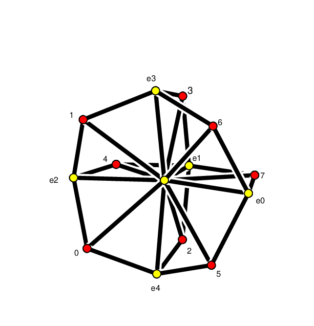
The tropical matroid polytope PP from Example 6 is contained in the 44-dimensional tropical hyperplane with apex 𝟎\mathbf{0}. It is shown in Figure 2 as the abstract graph of the vertices and edges of its bounded subcomplex. Its maximal bounded cells are ordinary simplices of dimension d−k+1=2d-k+1=2, whose pseudovertices are the tropical vertices V={vB1,…,vB8}V=\{v_{B_{1}},\ldots,v_{B_{8}}\} (dark), the origin 𝟎\mathbf{0} (the centered point) and the five corners ci=eic_{i}=e_{i} (light). The four tropical vertices with indices 33, 44, 55 and 88 correspond to the bases that are possible after deleting edge 11 in the underlying graph and therefore adjacent to the point e1e_{1}. One valid sequence i1,i2i_{1},i_{2} leading to a maxim bounded cell is for example the (tropical/ordinary) convex hull of e∅=(0,0,0,0,0),e4=(0,0,0,0,1)e_{\emptyset}=(0,0,0,0,0),\,e_{4}=(0,0,0,0,1) and e4,2=vB1=(0,0,1,0,1)e_{4,2}=v_{B_{1}}=(0,0,1,0,1), i.e. i1=4i_{1}=4 and i2=2i_{2}=2, with interior cell type (1,1,36,1,24578)(1,1,36,1,24578), representing the basis B1={1,2,4}B_{1}=\{1,2,4\}.

Figure 2. The abstract 1-skeleton of the bounded subcomplex of the tropical matroid polytope of Example 6.
Refer to caption

All cells in the tropical complex 𝒞V\mathcal{C}_{V}, bounded or not, are pointed, i.e. they do not contain an affine line. So each cell of 𝒞V\mathcal{C}_{V} must contain a bounded cell as an ordinary face.

We now state the main theorem about the coarse types of maximal cells in the cell complex of a tropical matroid polytope. Let bI,Jb_{I,J} denote the number of bases B∈ℬB\in\mathcal{B} with I⊆BI\subseteq B and J⊆BCJ\subseteq B^{C}.

Theorem 11.

Let 𝒞\mathcal{C} be the tropical complex induced by the tropical vertices of a tropical matroid polytope P∈𝒫k,dP\in\mathcal{P}_{k,d}. The set of all coarse types of the maximal cells arising in 𝒞\mathcal{C} is given by those tuples (t1,…,td+1)(t_{1},\ldots,t_{d+1}) with

(4) tj={b{i1},∅+b∅,{i1,i2,…,id′+1}if j=i1,b{il},{i1,…,il−1}if j=il∈{i2,…​id′+1},0otherwise.t_{j}\ =\ \begin{cases}b_{\{i_{1}\},\emptyset}+b_{\,\emptyset,\{i_{1},i_{2},\ldots,i_{d^{\prime}+1}\}}&\text{if $j=i_{1}$}\,,\\ b_{\{i_{l}\},\{i_{1},\ldots,i_{l-1}\}}&\text{if $j=i_{l}\in\{i_{2},\ldots i_{d^{\prime}+1}\}$}\,,\\ 0&\text{otherwise}\,.\end{cases}

where ei1,…,ei1,i2,…,id′e_{i_{1}},\ldots,e_{i_{1},i_{2},\ldots,i_{d^{\prime}}} form a subsequence of a valid sequence of PP.

Proof.

Depending on the maximal bounded (ordinary) face in the boundary, there are three types of maximal unbounded cells in 𝒞V\mathcal{C}_{V}.

The first one, XTX_{T}, contains a maximal bounded cell of dimension d−k+1d-k+1, which is the tropical convex hull of the pseudovertices of a complete valid sequence 𝟎,ei1,ei1,i2,…,ei1,i2,…,id−k+1\mathbf{0},e_{i_{1}},e_{i_{1},i_{2}},\ldots,e_{i_{1},i_{2},\ldots,i_{d-k+1}} where BC={i1,…,id−k+1}B^{C}=\{i_{1},\ldots,i_{d-k+1}\} is the complement of a basis of ℳ\mathcal{M}. To get full-dimensional we have the choice between k−1k-1 of kk free directions −ei-e_{i}, i∈Bi\in B. So let −ej1∞,…,−ejk−1∞-e^{\infty}_{j_{1}},\ldots,-e^{\infty}_{j_{k-1}} be the extreme rays of XTX_{T}, and (T1(0),…,Td+1(0))(T^{(0)}_{1},\ldots,T^{(0)}_{d+1}) be the type of the pseudovertex 𝟎\mathbf{0} with respect to PP. Then the type T=(T1,…,Td+1)T=(T_{1},\ldots,T_{d+1}) of the interior of this unbounded cell XTX_{T} is given by the intersection of the types of its vertices and therefore Ti1=Ti1(0),Ti2=Ti2(0)∖Ti1(0),…,Tid−k+1=Tid−k+1(0)∖(Ti1(0)∪Ti2(0)∪Tid−k(0))T_{i_{1}}=T^{(0)}_{i_{1}},T_{i_{2}}=T^{(0)}_{i_{2}}\setminus T^{(0)}_{i_{1}},\ldots,T_{i_{d-k+1}}=T^{(0)}_{i_{d-k+1}}\setminus(T^{(0)}_{i_{1}}\cup T^{(0)}_{i_{2}}\cup T^{(0)}_{i_{d-k}}), Ti=Ti(0)∖(Ti1(0)∪Ti2(0)∪Tid−k+1(0))T_{i}=T^{(0)}_{i}\setminus(T^{(0)}_{i_{1}}\cup T^{(0)}_{i_{2}}\cup T^{(0)}_{i_{d-k+1}}) for i∉BC∪{j1,…,jk−1}i\notin B^{C}\cup\{j_{1},\ldots,j_{k-1}\} and Tj1=…=Tjk−1=∅T_{j_{1}}=\ldots=T_{j_{k-1}}=\emptyset. Choosing d′=d−k+1d^{\prime}=d-k+1 and id′+1=ii_{d^{\prime}+1}=i, we get the coarse type entries of equation (4).

The second type, XTX_{T}, of maximal unbounded cells contains a bounded cell of lower dimension d′∈{0,…,d−k}d^{\prime}\in\{0,\ldots,d-k\}, which is the tropical convex hull of the pseudovertices of some subsequence ei1,ei1,i2,…,ei1,i2,…,id′+1e_{i_{1}},e_{i_{1},i_{2}},\ldots,e_{i_{1},i_{2},\ldots,i_{d^{\prime}+1}}. To get full-dimensional we still need the extreme rays ei1,i2,…,id′+1−el∞e_{i_{1},i_{2},\ldots,i_{d^{\prime}+1}}-e^{\infty}_{l} for all directions l∉{i1,…,id′+1}l\notin\{i_{1},\ldots,i_{d^{\prime}+1}\}. Then the type T=(T1,…,Td+1)T=(T_{1},\ldots,T_{d+1}) of the interior of this unbounded cell XTX_{T} is given by Ti1=Ti1(0)∪(Ti1(0)C∩⋯∩Tid′+1(0)C),Ti2=Ti2(0)∖Ti1(0),…,Tid′+1=Tid′+1(0)∖(Ti1(0)∪Ti2(0)∪Tid′(0))T_{i_{1}}=T^{(0)}_{i_{1}}\cup({T^{(0)}_{i_{1}}}^{C}\cap\cdots\cap{T^{(0)}_{i_{d^{\prime}+1}}}^{C}),T_{i_{2}}=T^{(0)}_{i_{2}}\setminus T^{(0)}_{i_{1}},\ldots,T_{i_{d^{\prime}+1}}=T^{(0)}_{i_{d^{\prime}+1}}\setminus(T^{(0)}_{i_{1}}\cup T^{(0)}_{i_{2}}\cup T^{(0)}_{i_{d^{\prime}}}), Tj=∅T_{j}=\emptyset for j∉{i1,…,id′+1}j\notin\{i_{1},\ldots,i_{d^{\prime}+1}\} with the coarse type as given in equation (4).

The third and last type of maximal unbounded cells contains a bounded cell of dimension d−kd-k and is assigned to the non-bases of ℳ\mathcal{M}, i.e. to the subsets of EE with cardinality kk that are not bases. Let i1,…,id−k+1i_{1},\ldots,i_{d-k+1} be the complement of a non-basis NN and i1,…,id−ki_{1},\ldots,i_{d-k} a valid subsequence. Then there is an unbounded cell XTX_{T} that is the tropical convex hull of the pseudovertices 𝟎,ei1,…,eid−k\mathbf{0},e_{i_{1}},\ldots,e_{i_{d-k}} and the extreme rays 𝟎−el∞\mathbf{0}-e^{\infty}_{l} for all directions l∉{i1,…,id−k+1}l\notin\{i_{1},\ldots,i_{d-k+1}\} and with type entries Ti1=Ti1(0),Ti2=Ti2(0)∖Ti1(0),…,Tid−k+1=Tid−k+1(0)∖(Ti1(0)∪Ti2(0)∪Tid−k(0))T_{i_{1}}=T^{(0)}_{i_{1}},T_{i_{2}}=T^{(0)}_{i_{2}}\setminus T^{(0)}_{i_{1}},\ldots,T_{i_{d-k+1}}=T^{(0)}_{i_{d-k+1}}\setminus(T^{(0)}_{i_{1}}\cup T^{(0)}_{i_{2}}\cup T^{(0)}_{i_{d-k}}), Tj=∅T_{j}=\emptyset for j∉{i1,…,id−k+1}j\notin\{i_{1},\ldots,i_{d-k+1}\}. Choosing d′=d−kd^{\prime}=d-k and observing that b∅,{i1,i2,…,id′+1}=0b_{\,\emptyset,\{i_{1},i_{2},\ldots,i_{d^{\prime}+1}\}}=0 for the non-basis {i1,i2,…,id′+1}C\{i_{1},i_{2},\ldots,i_{d^{\prime}+1}\}^{C} we get the desired result. ∎

Restricting ourselves to the uniform case, we get the following result.

Corollary 12.

The coarse types of the maximal cells in the tropical complex induced by the tropical vertices of the tropical hypersimplex Δkd\Delta_{k}^{d} in 𝕋d{\mathbb{T}}^{d} with 2≤k<d+12\leq k<d+1 are up to symmetry of Sym⁡(d+1)\operatorname{Sym}(d+1) given by

((d+1−αk)+(dk−1),(d−1k−1),…,(d−(α−1)k−1),0,…,0⏟d+1−α)\left(\binom{d+1-\alpha}{k}+\binom{d}{k-1},\,\binom{d-1}{k-1},\ldots,\,\binom{d-(\alpha-1)}{k-1},\underbrace{0,\ldots,0}_{d+1-\alpha}\right)

where 0≤α≤d+2−k0\leq\alpha\leq d+2-k correlates to the maximal dimension of a bounded cell of its boundary.

Now we relate the combinatorial properties of the tropical complex 𝒞\mathcal{C} of a tropical matroid polytope to algebraic properties of a monomial ideal which is assigned to 𝒞\mathcal{C}. As a direct consequence of Theorem 3 and Corollary 3.5 in [7], we can state the generators of the coarse type ideal

I=⟨x𝐭⁡(p):p∈𝕋d⟩⊂𝕂[x1,…,xd+1],I=\langle x^{\mathbf{t}(p)}\colon p\in{\mathbb{T}}^{d}\rangle\subset{\mathbb{K}}[x_{1},\ldots,x_{d+1}],

where 𝐭⁡(p)\mathbf{t}(p) is the coarse type of pp and x𝐭⁡(p)=x1𝐭​(p)1x2𝐭​(p)2⋯xd+1𝐭​(p)d+1x^{\mathbf{t}(p)}={x_{1}}^{{\mathbf{t}(p)}_{1}}{x_{2}}^{{\mathbf{t}(p)}_{2}}\cdots{x_{d+1}}^{{\mathbf{t}(p)}_{d+1}}.

Corollary 13.

The coarse type ideal II is equal to

⟨xi1ti1xi2ti2⋯xid′+1tid′+1:[d+1]∖{i1,…,id′} contains a basis ⟩\langle x_{i_{1}}^{t_{i_{1}}}x_{i_{2}}^{t_{i_{2}}}\cdots x_{i_{d^{\prime}+1}}^{t_{i_{d^{\prime}+1}}}\colon[d+1]\setminus\{i_{1},\ldots,i_{d^{\prime}}\}\text{ contains a basis }\rangle

with (ti1,ti2,…,tid′+1)=(b{i1},∅+b∅,{i1,i2,…,id′+1},b{i2},{i1},…,b{id′+1},{i1,…,id′})(t_{i_{1}},t_{i_{2}},\ldots,t_{i_{d^{\prime}+1}})=\big(b_{\{i_{1}\},\emptyset}+b_{\,\emptyset,\{i_{1},i_{2},\ldots,i_{d^{\prime}+1}\}},b_{\{i_{2}\},\{i_{1}\}},\ldots,b_{\{i_{d^{\prime}+1}\},\{i_{1},\ldots,i_{d^{\prime}}\}}\big).

Example 14.

The tropical complex 𝒞\mathcal{C} of the tropical matroid polytope of Example 6 has 73 maximal cells. There are five maximal cells for the case d′=0d^{\prime}=0 with tid′+1=8t_{i_{d^{\prime}+1}}=8 and tj=0t_{j}=0 for j≠id′+1j\neq i_{d^{\prime}+1}, and 48 for the case d′=2d^{\prime}=2 according to the 8 bases. Finally, there are 20 maximal cells for the case d′=1d^{\prime}=1, where [d+1]∖{i1}[d+1]\setminus\{i_{1}\} contains a basis, but [d+1]∖{i1,i2}[d+1]\setminus\{i_{1},i_{2}\} does not necessarily contain a basis.

The coarse type ideal of 𝒞\mathcal{C} is given by

I\displaystyle I =⟨\displaystyle=\langle x11​x22​x35,x11​x25​x32,x12​x21​x35,x14​x21​x33,x14​x23​x31,x12​x25​x31,x22​x36,x26​x32,\displaystyle{x_{1}}^{1}{x_{2}}^{2}{x_{3}}^{5},{x_{1}}^{1}{x_{2}}^{5}{x_{3}}^{2},{x_{1}}^{2}{x_{2}}^{1}{x_{3}}^{5},{x_{1}}^{4}{x_{2}}^{1}{x_{3}}^{3},{x_{1}}^{4}{x_{2}}^{3}{x_{3}}^{1},{x_{1}}^{2}{x_{2}}^{5}{x_{3}}^{1},{x_{2}}^{2}{x_{3}}^{6},{x_{2}}^{6}{x_{3}}^{2},
x22​x35​x41,x25​x32​x41,x12​x36,x15​x33,x12​x35​x41,x14​x33​x41,x38,x35​x43,x18,x15​x23,\displaystyle{x_{2}}^{2}{x_{3}}^{5}{x_{4}}^{1},{x_{2}}^{5}{x_{3}}^{2}{x_{4}}^{1},{x_{1}}^{2}{x_{3}}^{6},{x_{1}}^{5}{x_{3}}^{3},{x_{1}}^{2}{x_{3}}^{5}{x_{4}}^{1},{x_{1}}^{4}{x_{3}}^{3}{x_{4}}^{1},{x_{3}}^{8},{x_{3}}^{5}{x_{4}}^{3},{x_{1}}^{8},{x_{1}}^{5}{x_{2}}^{3},
x15​x43,x14​x31​x43,x14​x23​x41,x14​x21​x43,x02​x46,x48,x02​x11​x45,x01​x12​x45,x12​x46,\displaystyle{x_{1}}^{5}{x_{4}}^{3},{x_{1}}^{4}{x_{3}}^{1}{x_{4}}^{3},{x_{1}}^{4}{x_{2}}^{3}{x_{4}}^{1},{x_{1}}^{4}{x_{2}}^{1}{x_{4}}^{3},{x_{0}}^{2}{x_{4}}^{6},{x_{4}}^{8},{x_{0}}^{2}{x_{1}}^{1}{x_{4}}^{5},{x_{0}}^{1}{x_{1}}^{2}{x_{4}}^{5},{x_{1}}^{2}{x_{4}}^{6},
x01​x22​x45,x22​x46,x02​x21​x45,x11​x22​x45,x12​x21​x45,x02​x31​x45,x33​x45,x22​x31​x45,\displaystyle{x_{0}}^{1}{x_{2}}^{2}{x_{4}}^{5},{x_{2}}^{2}{x_{4}}^{6},{x_{0}}^{2}{x_{2}}^{1}{x_{4}}^{5},{x_{1}}^{1}{x_{2}}^{2}{x_{4}}^{5},{x_{1}}^{2}{x_{2}}^{1}{x_{4}}^{5},{x_{0}}^{2}{x_{3}}^{1}{x_{4}}^{5},{x_{3}}^{3}{x_{4}}^{5},{x_{2}}^{2}{x_{3}}^{1}{x_{4}}^{5},
x12​x31​x45,x01​x25​x42,x26​x42,x25​x31​x42,x11​x25​x42,x02​x36,x01​x22​x35,x02​x21​x35,\displaystyle{x_{1}}^{2}{x_{3}}^{1}{x_{4}}^{5},{x_{0}}^{1}{x_{2}}^{5}{x_{4}}^{2},{x_{2}}^{6}{x_{4}}^{2},{x_{2}}^{5}{x_{3}}^{1}{x_{4}}^{2},{x_{1}}^{1}{x_{2}}^{5}{x_{4}}^{2},{x_{0}}^{2}{x_{3}}^{6},{x_{0}}^{1}{x_{2}}^{2}{x_{3}}^{5},{x_{0}}^{2}{x_{2}}^{1}{x_{3}}^{5},
x02​x11​x35,x01​x12​x35,x02​x35​x41,x01​x25​x32,x03​x25,x28,x01​x12​x25,x12​x26,x12​x25​x41,\displaystyle{x_{0}}^{2}{x_{1}}^{1}{x_{3}}^{5},{x_{0}}^{1}{x_{1}}^{2}{x_{3}}^{5},{x_{0}}^{2}{x_{3}}^{5}{x_{4}}^{1},{x_{0}}^{1}{x_{2}}^{5}{x_{3}}^{2},{x_{0}}^{3}{x_{2}}^{5},{x_{2}}^{8},{x_{0}}^{1}{x_{1}}^{2}{x_{2}}^{5},{x_{1}}^{2}{x_{2}}^{6},{x_{1}}^{2}{x_{2}}^{5}{x_{4}}^{1},
x01​x14​x23,x06​x42,x05​x11​x42,x05​x12​x41,x03​x14​x41,x01​x14​x43,x05​x21​x42,x05​x23,\displaystyle{x_{0}}^{1}{x_{1}}^{4}{x_{2}}^{3},{x_{0}}^{6}{x_{4}}^{2},{x_{0}}^{5}{x_{1}}^{1}{x_{4}}^{2},{x_{0}}^{5}{x_{1}}^{2}{x_{4}}^{1},{x_{0}}^{3}{x_{1}}^{4}{x_{4}}^{1},{x_{0}}^{1}{x_{1}}^{4}{x_{4}}^{3},{x_{0}}^{5}{x_{2}}^{1}{x_{4}}^{2},{x_{0}}^{5}{x_{2}}^{3},
x05​x12​x21,x03​x14​x21,x05​x31​x42,x05​x21​x32,x05​x32​x41,x06​x32,x05​x11​x32,x06​x12,\displaystyle{x_{0}}^{5}{x_{1}}^{2}{x_{2}}^{1},{x_{0}}^{3}{x_{1}}^{4}{x_{2}}^{1},{x_{0}}^{5}{x_{3}}^{1}{x_{4}}^{2},{x_{0}}^{5}{x_{2}}^{1}{x_{3}}^{2},{x_{0}}^{5}{x_{3}}^{2}{x_{4}}^{1},{x_{0}}^{6}{x_{3}}^{2},{x_{0}}^{5}{x_{1}}^{1}{x_{3}}^{2},{x_{0}}^{6}{x_{1}}^{2},
x03x15,x05x12x31,x03x14x31,x08,x01x14x33⟩⊆R:=ℝ[x0,x1,x2,x3,x4]\displaystyle{x_{0}}^{3}{x_{1}}^{5},{x_{0}}^{5}{x_{1}}^{2}{x_{3}}^{1},{x_{0}}^{3}{x_{1}}^{4}{x_{3}}^{1},{x_{0}}^{8},{x_{0}}^{1}{x_{1}}^{4}{x_{3}}^{3}\,\rangle\subseteq R:={\mathbb{R}}[{x_{0}},{x_{1}},{x_{2}},{x_{3}},{x_{4}}]

We obtain its minimal free resolution, which is induced by 𝒞\mathcal{C}

ℱ∙𝒞: 0→R14→R78→R172→R180→R73→I→0,\mathcal{F}_{\bullet}^{\mathcal{C}}\colon\,0\rightarrow R^{14}\rightarrow R^{78}\rightarrow R^{172}\rightarrow R^{180}\rightarrow R^{73}\rightarrow I\rightarrow 0,

where the exponents ii of the free graded RR-modules RiR^{i} correspond to the entries of the ff-vector f⁡(𝒞)=(1,14,78,172,180,73)f(\mathcal{C})=(1,14,78,172,180,73) of 𝒞\mathcal{C}.

In (ordinary) convexity swapping between interior and exterior description of a polytope is a famous problem known as the convex hull problem. For a uniform matroid it is possible to indicate the minimal tropical halfspaces of its tropical matroid polytope.

Theorem 15.

The tropical hypersimplex Δkd\Delta_{k}^{d} in 𝕋d{\mathbb{T}}^{d} is the intersection of its cornered halfspaces and the tropical halfspaces H⁡(𝟎,I)H(\mathbf{0},I), where II is a (d−k+2)(d-k+2)-element subset of [d+1][d+1].

Proof.

For k=1k=1 the tropical standard simplex is a polytrope and coincides with its cornered hull. For k≥2k\geq 2 we want to verify the three conditions of Gaubert and Katz in Proposition 1 of [9].

Let T=(T1,…,Td+1)T=(T_{1},\ldots,T_{d+1}) be the type of the apex 𝟎\mathbf{0} of H⁡(𝟎,I)H(\mathbf{0},I). If a vertex v∈Vert⁡(Δkd)v\in\V(\Delta_{k}^{d}) appears in some type entry TiT_{i}, then the ii-th (canonical) coordinate of vv is equal to zero. Hence, exactly kk entries of TT contain the index of vv. Since the cardinality of IC=[d+1]∖II^{C}=[d+1]\setminus I is only k−1k-1, every tropical vertex of Δkd\Delta_{k}^{d} is contained in some sector Si¯\overline{S_{i}} with i∈Ii\in I, i.e. Δkd⊆H⁡(𝟎,I)\Delta_{k}^{d}\subseteq H(\mathbf{0},I).

Consider the complement ICI^{C} of II. For all i∈ICi\in I^{C} there is a tropical vertex vv with vi=0v_{i}=0, i.e. v∈Tiv\in T_{i}. Since the cardinality of ICI^{C} is equal to k−1k-1 and vv has kk entries equal to zero, there must be an index j∈Ij\in I such that vj=0v_{j}=0. We can conclude that Ti∩Tj≠∅T_{i}\cap T_{j}\neq\emptyset.

The intersection Ti∩TjT_{i}\cap T_{j} is not empty for arbitrary i,j∈[d+1]i,j\in[d+1], because its cardinality is equal to the number of tropical vertices vv with vi=vj=0v_{i}=v_{j}=0, which is (dk−1)\binom{d}{k-1} with k>1k>1. For i∈Ii\in I and j∈ICj\in I^{C}, the set Ti∩TjT_{i}\cap T_{j} consists of all tropical vertices vv with vi=0v_{i}=0 and vj=1v_{j}=1 (in canonical coordinates). On the other hand, the set ⋃k∈I∖{i}Tk\bigcup_{k\in I\setminus\{i\}}T_{k} contains all tropical vertices vv with vi=1v_{i}=1. So we get Ti∩Tj⊄⋃k∈I∖{i}TkT_{i}\cap T_{j}\not\subset\bigcup_{k\in I\setminus\{i\}}T_{k}.

Hence, we obtain that H⁡(𝟎,I)H(\mathbf{0},I) is a minimal tropical halfspace, and Δkd\Delta_{k}^{d} is contained in the intersection of its cornered hull ⋂i∈[d+1]H⁡(ei,{i})\displaystyle\bigcap_{i\in[d+1]}H(e_{i},\{i\}) with ⋂I∈([d+1]d−k+2)H⁡(𝟎,I)\displaystyle\bigcap_{I\in\binom{[d+1]}{d-k+2}}H(\mathbf{0},I).

We still have to prove that the intersection of the given minimal tropical halfspaces is contained in Δkd\Delta_{k}^{d}. Let us assume that there is a point x∈𝕋d∖Δkdx\in{\mathbb{T}}^{d}\setminus\Delta_{k}^{d} with typeΔkd⁡(x)i=∅\operatorname{type}_{\Delta_{k}^{d}}(x)_{i}=\emptyset. Then for any tropical halfspace H⁡(𝟎,I)H(\mathbf{0},I), I∈([d+1]d−k+2)I\in\binom{[d+1]}{d-k+2}, with i∈ICi\in I^{C} we obtain x∉H⁡(𝟎,I)x\notin H(\mathbf{0},I).

Consequently, the tropical hypersimplex Δkd\Delta_{k}^{d} is the set of all points x∈𝕋dx\in{\mathbb{T}}^{d} satisfying

⨁i∈Ixi\displaystyle\displaystyle\bigoplus_{i\in I}x_{i} ≤\displaystyle\leq ⨁j∈ICxj for all I⊆[d+1] with |I|=d−k+2\displaystyle\bigoplus_{j\in I^{C}}x_{j}\text{ for all }I\subseteq[d+1]\text{ with }\lvert I\rvert=d-k+2
and ​(−1)⊙xi\displaystyle\text{and }(-1)\odot x_{i} ≤\displaystyle\leq ⨁j≠ixj​ for all ​i∈[d+1].\displaystyle\bigoplus_{j\neq i}x_{j}\text{ for all }i\in[d+1].

∎

Example 16.

The second tropical hypersimplex Δ23\Delta_{2}^{3} in 𝕋3{\mathbb{T}}^{3} is the intersection of the 44 cornered halfspaces (ci,{i})(c_{i},\{i\}) for i=1,…,4i=1,\ldots,4 and the tropical halfspaces (𝟎,{1,2,3})(\mathbf{0},\{1,2,3\}), (𝟎,{1,2,4})(\mathbf{0},\{1,2,4\}), (𝟎,{1,3,4})(\mathbf{0},\{1,3,4\}) and (𝟎,{2,3,4})(\mathbf{0},\{2,3,4\}) with apex 𝟎∈𝕋d\mathbf{0}\in{\mathbb{T}}^{d}. The second tropical hypersimplex Δ22\Delta_{2}^{2} in 𝕋2{\mathbb{T}}^{2} is the intersection of the three cornered halfspaces (ci,{i})(c_{i},\{i\}) for i=1,…,3i=1,\ldots,3 and the tropical halfspaces (𝟎,{1,2})(\mathbf{0},\{1,2\}), (𝟎,{1,3})(\mathbf{0},\{1,3\}) and (𝟎,{2,3})(\mathbf{0},\{2,3\}) with apex 𝟎∈𝕋2\mathbf{0}\in{\mathbb{T}}^{2}, see Figure 3.

Refer to caption
(a)
Refer to caption
(b)
Figure 3. The tropical hypersimplex Δ22\Delta_{2}^{2} (dark) is given as the intersection of its cornered halfspaces (light coloured in Figure 3(a)) and the minimal tropical halfspaces (𝟎,{1,2})(\mathbf{0},\{1,2\}), (𝟎,{1,3})(\mathbf{0},\{1,3\}) (light coloured in Figure 3(b)).

Acknowledgements. I would like to thank my advisor Michael Joswig for suggesting the problem, and for supporting me writing this article.

References

  • [1] Dave Bayer, Irena Peeva, and Bernd Sturmfels, Monomial resolutions, Math. Res. Lett. 5 (1998), no. 1-2, 31–46.
  • [2] Dave Bayer and Bernd Sturmfels, Cellular resolutions of monomial modules, J. Reine Angew. Math. 502 (1998), 123–140.
  • [3] Florian Block and Josephine Yu, Tropical convexity via cellular resolutions, J. Algebraic Combin. 24 (2006), no. 1, 103–114.
  • [4] Mike Develin, Francisco Santos, and Bernd Sturmfels, On the rank of a tropical matrix, Combinatorial and computational geometry, Math. Sci. Res. Inst. Publ., vol. 52, Cambridge Univ. Press, Cambridge, 2005, pp. 213–242.
  • [5] Mike Develin and Bernd Sturmfels, Tropical convexity, Doc. Math. 9 (2004), 1–27 (electronic), correction: ibid., pp. 205–206.
  • [6] Mike Develin and Josephine Yu, Tropical polytopes and cellular resolutions, Experiment. Math. 16 (2007), no. 3, 277–291.
  • [7] Anton Dochtermann, Michael Joswig, and Raman Sanyal, Tropical types and associated cellular resolutions, 2010, preprint arXiv.org:1001.0237.
  • [8] Jack Edmonds, Submodular functions, matroids, and certain polyhedra, Combinatorial optimization—Eureka, you shrink!, Lecture Notes in Comput. Sci., vol. 2570, Springer, Berlin, 2003, pp. 11–26.
  • [9] Stephane Gaubert and Ricardo D. Katz, Minimal half-spaces and external respresentation of tropical polyhedra, J. Algebraic Combin. (2010), 1–24, 10.1007/s10801-010-0246-4.
  • [10] I. M. Gel′fand, R. M. Goresky, R. D. MacPherson, and V. V. Serganova, Combinatorial geometries, convex polyhedra, and Schubert cells, Adv. in Math. 63 (1987), no. 3, 301–316.
  • [11] Michael Joswig, Tropical halfspaces, Combinatorial and computational geometry, Math. Sci. Res. Inst. Publ., vol. 52, Cambridge Univ. Press, Cambridge, 2005, pp. 409–431.
  • [12] by same author, Tropical convex hull computations, Tropical and idempotent mathematics, Contemp. Math., vol. 495, Amer. Math. Soc., Providence, RI, 2009, pp. 193–212.
  • [13] Michael Joswig and Katja Kulas, Tropical and ordinary convexity combined, Advances in Geometry 10 (2010), 333–352.
  • [14] Michael Joswig, Bernd Sturmfels, and Josephine Yu, Affine buildings and tropical convexity, Albanian J. Math. 1 (2007), no. 4, 187–211.
  • [15] James Oxley, What is a matroid?, Cubo Mat. Educ. 5 (2003), no. 3, 179–218.
  • [16] Neil White (ed.), Theory of matroids, Encyclopedia of Mathematics and its Applications, vol. 26, Cambridge University Press, Cambridge, 1986.
  • [17] by same author, Combinatorial geometries, Encyclopedia of Mathematics and its Applications, vol. 29, Cambridge University Press, Cambridge, 1987.
  • [18] by same author, Matroid applications, Encyclopedia of Mathematics and its Applications, vol. 40, Cambridge University Press, Cambridge, 1992.