Bulk viscous cosmology: unified dark matter
Abstract
The bulk viscosity is introduced to model unified dark matter. The viscous unified model assumes the universe is filled with a single fluid with the bulk viscosity. We review the general framework of the viscous cosmology. The Hubble parameter has a direct connection with the bulk viscosity coefficient. For concrete form of the bulk viscosity, the Hubble parameter which has the scaling relation with the redshift can be obtained. We discuss two viscosity models and the cosmological evolution to which they lead. Using SNe Ia data, the viscosity model can be fitted. We briefly review the fitting method here.
I Introduction
Both dark matter problem and the cosmic acceleration problem challenge physicists’ understanding of the universe. In the standard CDM model, two mixed fluids, dark matter and dark energy fluid, are assumed. These two fluids influence the cosmic evolution separately. However, present gravitational probe does not have the ability to differentiate these two fluids. This is the dark degeneracy problem [1] [2]. It is reasonable to model dark matter and dark energy with single fluid or single field assumption. Some unified models have been proposed to detect the possibility of this unified assumption, like unified dark fluid model [3] [4] [5] [6] [7], which assumes the single fluid equation of state; Chaplygin gas model and generalized Chaplygin gas [9] [10] [11] [12] [13], which discuss the cosmology consequences of an exotic equation of state; scalar field method [14] [15] [16].
The introduction of viscosity into cosmology has been investigated from different view points [17] [18]. There are some recent developments like dark energy model [19] [20] [21] [22], the cosmic singularity [23]. In this review, we give a brief introduction to unify dark matter and dark energy with viscosity medium. In such models, the universe is assumed to be filled with viscous single fluid [24] [25] [26] [27] [28] [29] [30]. The cosmic density is not separated as dark energy part and dark matter part. The bulk viscosity contributes to the cosmic pressure, and plays the role as accelerating the universe. After considering the bulk viscosity, the cosmic pressure can be written as
| (1) |
Where parameterizes the equation of state. Generally the form of bulk viscosity is chosen as a time-dependent function. In [31] [32] [33] [34], a density-dependent viscosity coefficient is investigated extensively. For modeling the unified dark matter and dark energy, it is often assumed that the parameter , that the pressure of the viscosity fluid is zero and the viscosity term contributes an effective pressure. There raises some problems here. From the observational results [35], the cosmic density nearly equals to the cosmic pressure. In the viscosity model, the viscosity term dominates the cosmic pressure, and surpasses the pressure contributions from other cosmic matter constitutions, which contradicts the traditional fluid theory. [36] [37] propose non-standard interaction mechanism to solve this problem. Obviously, it is important to build solid foundation for the research of the viscous cosmology.
Equation of state lies in the phantom region. It is shown that cosmology models with such equation of state possess the so-called the future singularity called the Big Rip [38]. The larger viscosity model parameter space can help to solve the cosmic singularity problem and produces different kinds of evolution mode of the future universe, for more details [29].
The rest of this review is organized as follows: In the next chapter, general framework of the viscosity model will be reviewed. In Sec. III, we discuss the modeling of the unified model with viscosity. In this section, two concrete models are analyzed. In Sec. IV, data fitting method is introduced briefly.
II General framework
We consider the standard Friedmann-Robertson-Walker metric,
| (2) |
For the sake of simplicity, we choose the flat geometry , which is also favored by the update result of the cosmic background radiation measurement.
The general stress-energy-momentum tensor is
| (3) |
where is the bulk viscosity. The expansion factor is defined by , and the projection tensor . In the co-moving coordinates, the four velocity . We do not specify the concrete form of in this section. Generally speaking, is a quantity evolving with time or the scale factor . We will see below that non-trivial and more complicated can produce different results especially useful for the late universe modeling.
From the usual Einstein equation,
| (4) |
we obtain two equations which we call the modified Friedmann equations:
| (5a) | |||||
| (5b) | |||||
where is an effective pressure, .
The covariant conservation equation yields
| (6) |
The existence of a bulk viscosity contributes a modification to the pressure , thus we see the Friedmann equation and the covariant conservation equation are invariant under the transformation
| (7) |
The covariant energy conservation equation becomes
| (8) |
If define the dimensionless Hubble parameter here
| (9) |
where is the critical density now. Using the dimensionless Hubble parameter, Eq. (8) can be transformed as
| (10) |
where the bulk viscosity is redefined as . Through the simple relation between scale factor and the redshift
| (11) |
we transform Eq. (10) into a differential equation with respect to the scale factor
| (12) |
Solving this equation, we obtain a integral form of
| (13) |
Different forms of viscosity can be used here to make this integral calculable, numerically or exactly.
III Unified single fluid
III.1 Redshift-dependent model
In [39], authors assume the bulk viscosity takes the form as an Hubble parameter dependent function. A redshift-dependent viscosity is proposed in [28]. This bulk viscosity is a combination of a constant and a scaling relation term
| (14) |
where is an integer, and are two constants, which will be fitted from the observational data sets.
After taking account of this ansatz, the integration is easily to work out. We get
| (15) |
Since we have assumed the spatial flat of the universe, the consistency condition requires . Thus this sets a constraint on the model parameters as
| (16) |
We remind the readers that we make the single fluid assumption above, and we do not concretely specify the constitutions of the cosmic density . In this single fluid model, values of model parameters , and will be fitted, and their meaning are not explained. But when we compare it with two-fluid model, that the universe is filled with dark matter and dark energy fluid, more constraints can be added. The solution consists terms with different scaling relation. The first term has the form like , which have the same evolution behavior as the cold dark matter. Their simplicity leads us to correspond parameter to dark matter ratio
| (17) |
This identity can help us utilize more data to constrain the viscosity model. The result is also consistent with that obtained from the standard model(CDM). The shift parameter [40] [41] and the distance parameter is defined as
| (18) |
and
| (19) |
respectively. Both of them are dependent on dark matter ratio , and in the joint statistical analysis they provide strong constraint on .
III.2 Effective equation of state model
Another viscosity model reviewed here is proposed in [26], where a general form time-dependent viscosity is discussed
| (20) |
An interesting feature of this model is its effective equivalence to the following equation of state
| (21) |
where , , and are free parameters. The corresponding between two groups of coefficients are
| (22a) | |||||
| (22b) | |||||
| (22c) | |||||
The parameterized bulk viscosity combines terms related to the “velocity” and “acceleration” , which can be seen to describe the dynamics of the cosmic non-perfect fluid. After eliminating and , a differential equation about the scale factor can be obtained
| (23) |
Another feature of this model is that this differential equation can be solved exactly, and the evolution function of the scale factor is definite. This evolution function is especially convenient for discussing the cosmic singularity.
With the initial conditions and , when , the scale factor can be obtained as
| (24) | |||||
where the parameters are redefined as
| (25) |
| (26) |
| (27) |
| (28) |
From Friedmann equation, can be written as
| (29) |
The model parameters leave enough space to produce various evolution behavior, which can be interpreted in different ways. In this review, we emphasis its power to unify dark energy and dark matter with the single fluid assumption. According to the parameters redefined above and the Friedmann equation, the equation of state can be converted to
| (30) |
The case and corresponds to the CDM. With the aim to unify dark energy and dark matter, the case and is especially considered. This case corresponds to a single fluid with constant viscosity. The relation between and can be obtained from the general equation of state above
| (31) |
Therefore, it is straightforward to eliminate from the covariant energy conservation equation, and to work out the solution of . Using Friedmann equation, can be obtained
| (32) |
is the only one model parameter. Its value can be fitted from SNe Ia observational data.
IV data fitting
We review the method to fit the model parameters. More details are illustrated in [42]. The data sets we use are SNe Ia, BAO and CMB. The 397 Constitution sample [43] combines the Union sample [44] and the low redshift () sample [45]. The co-moving distance in FRW coordinate is
| (33) |
The apparent magnitude which is measured is
| (34) |
where the dimensionless luminosity and
| (35) |
where is the absolute magnitude which is believed to be constant for all SNe Ia. In the SNe Ia samples, data are given in terms of the distance modulus . The for this procedure is written as
| (36) |
where means the distance modulus calculated from model with parameters (). Together with the shift parameter and the distance , the total for the joint data analysis is
| (37) |
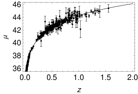
For the redshift-dependent model, the relation between distance modulus and redshift is plotted in FIG.1. The model calculated value and the Constitution data is compared in the figure.
V conclusion
In this review, we discuss three aspects of the viscosity model,
- •
General framework for viscosity modeling. General form of Hubble parameter is presented. This general form is convenient for comparing different scale factor(or redshift) dependent viscosity models.
- •
Two kinds of viscosity models are used to model unified models.
- •
Observation constraint is necessary for model building. We can see the fitting results are consistent with data. It is prospected that more accurate direct measurements of Hubble constant will provide a new constraint on cosmological parameters [46].
Especially we focus on its application on modeling the unified dark energy and dark matter.
In the cosmic background level, dynamical analysis can be performed. The statefinder method is useful for discriminating different models [47] [48] [49] [50] [51]. Compared with CDM model, evolution of the statefinder of the viscosity model is different and can be discriminated easily, more details can be found in [52] [29]. More plentiful and accurate data will improve the power of the statefinder method, which will give enough constraint on the late universe model.
We review the viscosity model which is on the level of zero order. The perturbation analysis and the large scale structure are especially useful for the model building. The model predictions need to be consistent with CMB and LSS data. Some works has investigated the perturbation aspects of the viscosity model [53] [34]. After corresponding the model parameters, the viscosity model has the connection with the Chaplygin gas model. Though the Chaplygin gas model can fit the SNe Ia data well, in the perturbation level it is found the Chaplygin gas model does not behave in a satisfactory way. Whether the viscosity models could behave well needs further investigation.
Acknowledgements
This work is supported in part by the National Science Foundation of China.
References
- [1] W. Hu and D.J. Eisenstein, Phys. Rev. D 59, 083509 (1999), arXiv:astro-ph/9809368.
- [2] M. Kunz, arXiv:astro-ph/0702615.
- [3] A. Balbi, M. Bruni and C. Quercellini, Phys. Rev. D 76 (2007) 103519, arXiv:astro-ph/0702423.
- [4] C. Quercellini, M. Bruni and A. Balbi, Class. Quant. Grav. 24 (2007) 5413, arXiv:0706.3667.
- [5] D. Pietrobon, A. Balbi, M. Bruni and C. Quercellini, Phys. Rev. D 78 (2008) 083510, arXiv:0807.5077.
- [6] M. Kunz, A.R. Liddle, D. Parkinson and C. Gao, Phys. Rev. D 80 (2009) 083533, arXiv:0908.3197.
- [7] A. Arbey, arXiv:astro-ph/0506732.
- [8] I. Brevik, E. Elizalde, O. Gorbunova and A. V. Timoshkin, Eur. Phys. J. C 52 (2007) 223-228, arXiv:0706.2072.
- [9] J.D. Barrow, Phys. Lett. B 235 (1990) 40.
- [10] M.C. Bento, O. Bertolami, A.A. Sen, Phys. Rev. D 66 043507 (2002), arXiv:gr-qc/0202064.
- [11] Zong-Hong Zhu, arXiv:astro-ph/0411039.
- [12] L. Amendola, F. Finelli, C. Burigana and D. Carturan, JCAP 07 (2003) 005, arXiv:astro-ph/0304325.
- [13] Xin-He Meng, Ming-Guang Hu and Jie Ren, arXiv:astro-ph/0510357.
- [14] S. Nojiri and S.D. Odintsov, Phys. Rev. D 72 (2005) 023003, arXiv:hep-th/0505215
- [15] S. Nojiri and S.D. Odintsov, Gen. Rel. Grav. 38 (2006) 1285-1304, arXiv:hep-th/0506212.
- [16] S. Capozziello, S. Nojiri and S.D. Odintsov, Phys. Lett. B 632 (2006) 597-604, arXiv:hep-th/0507182.
- [17] Ø. Grøn, Astrophys. Space Sci. 173 (1990) 191.
- [18] T. Padmanabhan and S. Chitre, Phys. Lett. A 120 (1987) 433.
- [19] I. Brevik and O. Gorbunova, Gen. Rel. Grav. 37 (2005) 2039, arXiv:gr-qc/0504001.
- [20] I. Brevik, arXiv:gr-qc/0404095.
- [21] C.J. Feng and X.Z. Li, Phys. Lett. B 680 (2009) 355-358, arXiv:0905.0527.
- [22] A. Avelino and U. Nucamendi, arXiv:1002.3605v1.
- [23] I. Brevik, arXiv:0811.1129.
- [24] X.H. Meng, J. Ren and M.G. Hu, Commun. Theor. Phys. 47 (2007) 379.
- [25] J. Ren and X.H. Meng, Int. J. Mod. Phys. D 16 (2007) 1341-1348, arXiv:astro-ph/0605010.
- [26] J. Ren and X.H. Meng, Phys. Lett. B 633 (2006) 1-8, arXiv:astro-ph/0511163.
- [27] J. Ren and X.H. Meng, Phys. Lett. B 636 (2006) 5-12, arXiv:astro-ph/0602462.
- [28] X. Dou and X.H. Meng, Commun. Theor. Phys. 52 (2009) 377-382, arXiv:0812.4904.
- [29] X.H. Meng and X. Dou, arXiv:0910.2397.
- [30] A. Avelino and U. Nucamendi, JCAP 0904 (2009) 006, arXiv:0811.3253v2.
- [31] J. Barrow, Phy. Lett. B 180 (1986) 335; J. Barrow, Nucl. Phys. B 310 (1988) 743; J. Barrow, in The Formation and Evolution of Cosmic Strings, eds. G. Gibbons and T. Vasasparti, p449-464, Cambridge University Press, Cambridge,UK.
- [32] B. Li and J.D. Barrow, Phys. Rev. D 79 (2009) 103521, arXiv:0902.3163.
- [33] R. Colistete Jr., J.C. Fabris, J. Tossa and W. Zimdahl, Phys. Rev. D 76 (2007) 103516, arXiv:0706.4086.
- [34] W.S. Hipolito-Ricaldi, H.E.S. Velten and W. Zimdahl, JCAP 0906 (2009) 016, arXiv:0902.4710.
- [35] E. Komatsu et al., arXiv:1001.4538.
- [36] W. Zimdahl, D. J. Schwarz, A. B. Balakin and D. Pavón, Phys. Rev. D 64 (2001) 063501, arXiv:astro-ph/0009353.
- [37] A.B. Balakin, D. Pavón, D.J. Schwarz and W. Zimdahl, NJP 5 (2003) 85.1.
- [38] R.R. Caldwell, M. Kamionkowski, and N.N. Weinberg, Phy. Rev. Lett. 91 (2003) 071301, arXiv:astro-ph/0302506.
- [39] V. Folomeev and V. Gurovich, Phys. Lett. B 661 (2008) 75-77, arXiv:0710.0210.
- [40] J. R. Bond, G. Efstathiou and M. Tegmark, Mon. Not. Roy. Astron. Soc. 291 (1997) L33, arXiv:astro-ph/9702100.
- [41] Y. Wang and P. Mukherjee, Astrophys. J. 650 (2006) 1, arXiv:astro-ph/0604051.
- [42] M.C. Bento, O. Bertolami, N.M.C. Santos and A.A. Sen, Phys. Rev. D 71 (2005) 063501.
- [43] M. Hicken et al., Astrophys. J. 700 (2009) 1097-1140, arXiv:0901.4804.
- [44] M. Kowalski et al. Astrophys. J. 686 (2008) 749-778, arXiv:0804.4142.
- [45] M. Hicken et al., Astrophys. J. 700 (2009) 331-357, arXiv:0901.4787.
- [46] L. Greenhill et al., arXiv:0902.4255.
- [47] V. Sahni, T.D. Saini, A.A. Starobinsky and U. Alam, JETP Lett. 77 (2003) 201, arxiv: astro-ph/0201498.
- [48] U. Alam, V. Sahni, T.D. Saini and A.A. Starobinsky, Mon. Not. R. Astron. Soc. 344 (2003) 1057, arxiv: astro-ph/0303009.
- [49] V. Gorini, A. Kamenshchik and U. Moschella, Phys. Rev. D 67 (2003) 063509, arxiv: astro-ph/0209395.
- [50] W. Zimdahl and D. Pavón, Gen. Relativ. Gravit. 36 (2004) 1483, arxiv: gr-qc/0311067.
- [51] V. Sahni, A. Shafieloo and A.A. Starobinsky, Phys. Rev. D 78 (2008) 103502, arXiv:0807.3548.
- [52] M.G. Hu and X.H. Meng, Phys. Lett. B 635 (2006) 186-194, arXiv:astro-ph/0511615.
- [53] J.C. Fabris, S.V.B. Goncalves and R. de Sa Ribeiro, Gen. Rel. Grav. 38 (2006) 495-506, arXiv:astro-ph/0503362.