跳到论文正文
W Papers独立论文阅读器 arXiv:1012.2958 论文正文 计算阅读时间 · 0%
引用这篇论文根据当前论文元数据生成,正式投稿前建议核对。


License: arXiv.org perpetual non-exclusive license
arXiv:1012.2958v2 [astro-ph.CO] 02 Mar 2011

The seed magnetic field generated during recombination

Elisa Fenu1 Affiliation: 1{}^{1}\,Université de Genève, Département de Physique Théorique, CH-1211 Genève, Switzerland
2{}^{2}\,Institute of Cosmology & Gravitation, University of Portsmouth, Portsmouth PO1 3FX, United Kingdom
3{}^{3}\,Department of Physics, University of Western Cape, Cape Town 7535, South Africa
   Cyril Pitrou2 Affiliation: 1{}^{1}\,Université de Genève, Département de Physique Théorique, CH-1211 Genève, Switzerland
2{}^{2}\,Institute of Cosmology & Gravitation, University of Portsmouth, Portsmouth PO1 3FX, United Kingdom
3{}^{3}\,Department of Physics, University of Western Cape, Cape Town 7535, South Africa
   Roy Maartens2,3 Affiliation: 1{}^{1}\,Université de Genève, Département de Physique Théorique, CH-1211 Genève, Switzerland
2{}^{2}\,Institute of Cosmology & Gravitation, University of Portsmouth, Portsmouth PO1 3FX, United Kingdom
3{}^{3}\,Department of Physics, University of Western Cape, Cape Town 7535, South Africa
August 24, 2026
Abstract

Nonlinear dynamics creates vortical currents when the tight-coupling approximation between photons and baryons breaks down around the time of recombination. This generates a magnetic field at second order in cosmological perturbations, whose power spectrum is fixed by standard physics, without the need for any ad hoc assumptions. We present the fully general relativistic calculation of the magnetic power spectrum, including the effects of metric perturbations, second-order velocity and photon anisotropic stress, thus generalizing and correcting previous results. We also show that significant magnetogenesis continues to occur after recombination. The power spectrum k3​PB\sqrt{k^{3}P_{B}} decays as k4k^{4} on large scales, and grows as k0.5k^{0.5} on small scales, down to the limit of our numerical computations, ∼1\sim 1\,Mpc. On cluster scales, the created field has strength ∼3×10⁻²⁹\sim 3\times 10^{-29}\,Gauss.

pacs
98.80.-k,98.58.Ay

I Introduction

Evidence is growing for magnetic fields on larger and larger scales in the Universe (see e.g. the reviews [1, 2]). In galaxies, the fields have strength of order μ\muGauss, ordered on scales ∼1−10\sim 1-10\,kpc. Fields of strength ∼1−10−2​μ\sim 1-10^{-2}\muG on scales ∼0.1−1\sim 0.1-1\,Mpc have been detected in galaxy clusters, and there is evidence of magnetic fields in superclusters. Recently, new evidence has been presented for intergalactic magnetic fields: high energy gamma-rays from distant sources can initiate electromagnetic pair cascades when interacting with the extragalactic photon background; the charged component of the cascades will be deflected by magnetic fields, affecting the images of the sources. Using observations from FERMI, a lower bound of order 10−1610^{-16}\,G has been claimed for the strength of fields in the filaments and voids of the cosmic web [3, 4, 5, 6].

The origin of these fields is still unclear (see e.g. [7, 8, 9]). They could have been generated via astrophysical processes during the nonlinear collapse stage of structure formation. There remain unresolved difficulties in explaining how these astrophysical seed fields lead to fields of the observed strength and coherence scales. Alternatively, the fields could be primordial seed fields – created in the very early Universe, during inflation, or during subsequent phase transitions. In principle inflation can generate fields on all scales – but unknown physics must be invoked to achieve non-minimal coupling of the electromagnetic field. The electroweak and QCD transitions can only produce fields on very small scales, up to the Hubble radius at magnetogenesis (and their amplitude is strongly constrained by their gravitational wave production before nucleosynthesis [10]).

Primordial magnetogenesis also takes place in the cosmic plasma after particle/anti-particle annihilation. This avoids the problem of exotic physics that faces inflationary magnetogenesis – standard Maxwell theory and standard cosmological perturbations in the cosmic plasma inevitably lead to magnetic fields. It also avoids the small coherence scale problem facing electroweak and QCD fields. However, the problem is the weakness of the fields, since this effect occurs at second and higher order in cosmological perturbations.

The key question is how weak is the field and how does it vary with scale? Differing qualitative estimates of the field strength have been given by [11, 12, 13, 14, 15, 16]. The power spectrum was first numerically computed by [17], which differs significantly from ours. More recently, [18] presented a power spectrum that is closer to our result. We discuss below the differences between previous results and ours. Our analysis is the first complete general relativistic computation of the power spectrum, taking into account all effects.

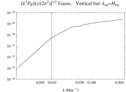
Our result is shown in Fig. 1. The power spectrum behaves as

k3​PB∝{k4k≪keqk0.5k≫keq.\sqrt{k^{3}P_{B}}\propto\left\{\begin{array}[]{ll}k^{4}&k\ll k_{\rm eq}\\ k^{0.5}&k\gg k_{\rm eq}\,.\end{array}\right. (1)

On cluster scales the comoving field strength is

B1​Mpc∼3×10⁻²⁹​G.B_{1\,{\rm Mpc}}\sim 3\times 10^{-29}\,{\rm G}. (2)
Refer to caption
Refer to caption
Figure 1: Left: Magnetic field spectrum today. Right: Comoving magnetic field strength today at a given scale.

Thus the field generated around recombination is too weak to act as a seed for the observed field strength of order μ\muG. Adiabatic contraction of the magnetic flux lines during nonlinear collapse of structures provides an enhancement of ∼103\sim 10^{3}, while the nonlinear dynamo mechanism has an amplification factor ∼108\sim 10^{8} (with many remaining uncertainties). Note that hydrodynamical and turbulence effects during nonlinear collapse themselves generate a field of order 10−2010^{-20}\,G – which is also too small to account for the observed galactic and cluster fields [8].

The field (2) is also too weak to imprint detectable effects on the CMB. Nevertheless it is a real property of the standard cosmological model, and may have some impact on early structure formation during the ‘dark ages’ if it is the only primordial field. (See e.g. [19, 20] for the role of magnetic fields in structure formation during the dark ages.)

As shown below, the magnetic field is given by

(a2​Bi)′\displaystyle\left(a^{2}B^{i}\right)^{\prime} =\displaystyle= −a2ϵi​j​k∂j[(1+Φ−Ψ)Ek],\displaystyle-a^{2}\epsilon^{ijk}\partial_{j}\Big[\left(1+\Phi-\Psi\right)E_{k}\Big], (3)
Ei\displaystyle E^{i} ≈\displaystyle\approx −4​ργ​σT3​e​(Δ​vb​γi+25​Θji​vbj),\displaystyle-\frac{4\rho_{\gamma}\sigma_{\mathrm{T}}}{3e}\Big(\Delta v_{{\mathrm{b}}\gamma}^{i}+\frac{2}{5}\Theta^{i}_{j}v_{{\mathrm{b}}}^{j}\Big), (4)

where Φ,Ψ\Phi,\Psi are first-order metric perturbations, Δ​vb​γi=vbi−vγi\Delta v_{{\mathrm{b}}\gamma}^{i}=v_{{\mathrm{b}}}^{i}-v_{\gamma}^{i} is the photon-baryon velocity difference, and Θji\Theta^{i}_{j} is the photon quadrupole moment, from anisotropic stress. This leads to three types of source terms for magnetogenesis:

(a2​B)′\displaystyle\left(a^{2}B\right)^{\prime} =\displaystyle= S1​[Δ​vb​γ(2)]+S2​[{δγ(1)+Φ(1)−Ψ(1)}​Δ​vb​γ(1)]\displaystyle S_{1}\big[\Delta v_{{\mathrm{b}}\gamma}^{(2)}\big]+S_{2}\big[\big\{\delta_{\gamma}^{(1)}+\Phi^{(1)}-\Psi^{(1)}\big\}\Delta v_{{\mathrm{b}}\gamma}^{(1)}\big] (5)
+S3​[Θγ(1)​vb(1)].\displaystyle~~+S_{3}\big[\Theta_{\gamma}^{(1)}v_{{\mathrm{b}}}^{(1)}\big].

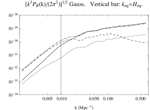
The first source term is second-order, while the other two are quadratic in first-order quantities. The contributions of the source terms to the power spectrum are shown in Fig. 5 (left).

Our paper builds on the physical analysis of nonlinear plasma dynamics presented in [21, 17, 18, 15, 22, 16, 23]. The key features of the dynamics are as follows.

  • •

    The electric field ensures that the proton-electron relative velocity is always strongly suppressed in comparison with the photon-electron relative velocity – even at high energies when the Compton interaction is stronger than the Coulomb interaction.

  • •

    Vorticity induced in the electron fluid is thus transferred almost entirely to the protons, and the baryon vorticity evolution is determined by the two-fluid dynamics of photons and baryons, which is very close to the equations of CMB dynamics. We use the second-order Boltzmann code of [23].

  • •

    The limit ve−vγ→0v_{\rm e}-v_{\rm\gamma}\to 0 and vp−ve→0v_{\rm p}-v_{\rm e}\to 0 is not equivalent to setting vp=ve=vγv_{\rm p}=v_{\rm e}=v_{\rm\gamma} in the momentum exchange equations, and the limit must be taken consistently.

  • •

    At first order, cosmological vector perturbations are zero after inflation, in the standard model. Magnetogenesis requires vortical currents, and these can therefore only be generated at second order, via mode-mode coupling of first-order scalar perturbations. This remains true even in the presence of topological defects, which are active sources for vector perturbations: at first order, the vector perturbations induced by the defects cannot break vorticity conservation in the cosmic plasma [24].

  • •

    On large scales there is some cancellation amongst the source terms in (5) (this is evident from Fig. 5). Neglecting any of the effects can thus lead to unreliable results.

  • •

    The magnetic field continues to be created after recombination, due to the residual nonzero ionization fraction. If the numerical integration is stopped at recombination, then the comoving field is under-estimated by a factor ∼10\sim 10 (see Fig. 5).

The plan of the paper is as follows. In the next section we review and clarify the magnetic and electric field generation beyond the tight-coupling limit. In Sec. III, we detail the numerical integration of the differential evolution equations at second order in cosmological perturbations that we perform in order to solve for the magnetic field spectrum. We also provide analytical insight into the time and scale behaviors of the numerical results. We compare our results with previous work in Sec. IV. Details of some calculations are given in the Appendices.

II Understanding the origin of the magnetic field

II.1 Interactions in the cosmic plasma

The stress-energy tensor of a species s{\mathrm{s}} satisfies

∇νTsμ​ν=∑rCsrμ,∑s∇νTsμ​ν=0,\nabla_{\nu}T_{{\mathrm{s}}}^{\mu\nu}=\sum_{\rm r}C^{\mu}_{{\mathrm{s}}{\rm r}}\,,~~\sum_{\mathrm{s}}\nabla_{\nu}T_{{\mathrm{s}}}^{\mu\nu}=0\,, (6)

where Csrν(=−Crsν)C^{\nu}_{{\mathrm{s}}{\rm r}}(=-C^{\nu}_{{\rm r}{\mathrm{s}}}) encodes all the effects of interactions with species rr. Relative to observers with 44-velocity uμu^{\mu}, the energy density transfer rate is −uμ​Csrμ-u_{\mu}C^{\mu}_{{\mathrm{s}}{\rm r}} and the momentum density transfer rate is Csrμ⟂=hνμ​CsrνC^{\mu\perp}_{{\mathrm{s}}{\rm r}}=h^{\mu}_{\nu}C^{\nu}_{{\mathrm{s}}{\rm r}}, where the projector is hμν≡δμν+uμ​uνh_{\mu}^{\nu}\equiv\delta_{\mu}^{\nu}+u_{\mu}u^{\nu}.

The Euler equation for a species s{\mathrm{s}} is given in general by

∇νTsν​μ⟂=∑rCsrμ⟂.\nabla_{\nu}T_{\mathrm{s}}^{\nu\mu\perp}=\sum_{\mathrm{r}}C^{\mu\perp}_{{\mathrm{s}}{\mathrm{r}}}\,. (7)

The kinematics of uμu^{\mu} are described by decomposing its covariant derivative as [21, 25]

∇μuν=13​θ​hμ​ν+σμ​ν+ωμ​ν−uμ​u˙ν,\nabla_{\mu}u_{\nu}={1\over 3}\theta h_{\mu\nu}+\sigma_{\mu\nu}+\omega_{\mu\nu}-u_{\mu}\dot{u}_{\nu}\,, (8)

where θ\theta is the volume expansion, σμ​ν\sigma_{\mu\nu} is the projected (i.e. orthogonal to uμu^{\mu}), symmetric and tracefree shear, ωμ​ν\omega_{\mu\nu} is the projected antisymmetric vorticity, and u˙μ=uν​∇νuμ\dot{u}_{\mu}=u^{\nu}\nabla_{\nu}u_{\mu} is the projected acceleration. The vorticity vector is defined as

ων≡ϵμ​ν​λ​ων​λ,ϵμ​ν​λ≡uτ​ϵτ​μ​ν​λ,\omega_{\nu}\equiv\epsilon_{\mu\nu\lambda}\omega^{\nu\lambda}\,,~~\epsilon_{\mu\nu\lambda}\equiv u^{\tau}\epsilon_{\tau\mu\nu\lambda}\,, (9)

where the totally antisymmetric tensor is defined by ϵ0123=−g\epsilon_{0123}=\sqrt{-g}. (Note that our sign convention for ωμ​ν\omega_{\mu\nu} and definition of ωμ\omega_{\mu} recover the Newtonian limit, and differ from [21, 25].)

In the period of interest, from the end of particle/anti-particle annihilation up to now (Tγ≲500​keVT_{\gamma}\lesssim 500{\rm keV}, z≲2×10⁹z\lesssim 2\times 10^{9}), the relevant species are protons, electrons, photons, and when recombination occurs, hydrogen atoms. Neutrinos affect only the background dynamics and the gravitational potentials in the Einstein equations. The Faraday tensor of the electromagnetic field defines electric and magnetic fields measured by uμu^{\mu} observers:

Eμ=Fμ​ν​uν,Bμ=12​ϵμ​ν​λ​Fν​λ.E^{\mu}=F^{\mu\nu}u_{\nu},~B^{\mu}=\frac{1}{2}\epsilon^{\mu\nu\lambda}F_{\nu\lambda}\,. (10)

Protons and electrons couple to the electromagnetic field through the term Cs​Fμ=Fνμ​jsνC^{\mu}_{{\mathrm{s}}F}=F^{\mu}_{\phantom{\mu}\nu}j_{\mathrm{s}}^{\nu}, where s=p,es={\mathrm{p}},{\mathrm{e}} and jsνj_{s}^{\nu} is the electric 4-current. Then ∇νTμ​νF=−∑sFμνjsν\nabla_{\nu}T^{\mu\nu}_{F}=-\sum_{\mathrm{s}}F^{\mu}_{\phantom{\mu}\nu}j_{\mathrm{s}}^{\nu}. We have jsμ=qs​ns​usμj_{\mathrm{s}}^{\mu}=q_{\mathrm{s}}n_{\mathrm{s}}u_{\mathrm{s}}^{\mu}, where qsq_{\mathrm{s}} is the particle charge, nsn_{\mathrm{s}} is the number density (in the rest frame) and the 4-velocity of species s{\mathrm{s}} is

usμ=γs(uμ+vsμ),uμvsμ=0,γs=(1−vs2)−1/2.u^{\mu}_{\mathrm{s}}=\gamma_{\mathrm{s}}(u^{\mu}+v_{\mathrm{s}}^{\mu}),~~u_{\mu}v_{\mathrm{s}}^{\mu}=0,~~\gamma_{\mathrm{s}}=\left(1-v_{\mathrm{s}}^{2}\right)^{-1/2}. (11)

Here γs​vsμ\gamma_{\mathrm{s}}v_{\mathrm{s}}^{\mu} is the relative velocity of s{\mathrm{s}} measured by uμu^{\mu}. Maxwell’s equations are given in Appendix A.

The momentum transfer rates are given by

Cpeμ⟂=−e2​ne​np​ηC​Δ​vpeμ,Δ​vpeμ≡γp​vpμ−γe​veμ,\displaystyle C^{\mu\perp}_{{\mathrm{p}}{\mathrm{e}}}=-e^{2}n_{{\mathrm{e}}}n_{{\mathrm{p}}}{\eta_{\rm C}}\Delta v^{\mu}_{{\mathrm{p}}{\mathrm{e}}}\,,~~\Delta v^{\mu}_{{\mathrm{p}}{\mathrm{e}}}\equiv\gamma_{{\mathrm{p}}}v_{{\mathrm{p}}}^{\mu}-\gamma_{{\mathrm{e}}}v_{{\mathrm{e}}}^{\mu}\,, (12)
Ce​γμ⟂=−43​ne​ργ​σT​(Δ​ve​γμ+25​Θνμ​veν),\displaystyle C^{\mu\perp}_{{\mathrm{e}}\gamma}=-\frac{4}{3}n_{{\mathrm{e}}}\rho_{\gamma}\sigma_{\mathrm{T}}\Big(\Delta v_{{\mathrm{e}}\gamma}^{\mu}+\frac{2}{5}\Theta^{\mu}_{\nu}v_{{\mathrm{e}}}^{\nu}\Big), (13)
Cp​γμ⟂=−43​β2​np​ργ​σT​(Δ​vp​γμ+25​Θνμ​vpν),β≡memp,\displaystyle C^{\mu\perp}_{{\mathrm{p}}\gamma}=-\frac{4}{3}\beta^{2}n_{{\mathrm{p}}}\rho_{\gamma}\sigma_{\mathrm{T}}\Big(\Delta v_{{\mathrm{p}}\gamma}^{\mu}+\frac{2}{5}\Theta^{\mu}_{\nu}v_{{\mathrm{p}}}^{\nu}\Big),~\beta\equiv{m_{{\mathrm{e}}}\over m_{{\mathrm{p}}}}, (14)
Cs​Fμ⟂=qsns(Eμ+ϵμ​ν​τvsνBτ),s=e,p.\displaystyle C^{\mu\perp}_{{\mathrm{s}}F}=q_{\mathrm{s}}n_{{\mathrm{s}}}\big(E^{\mu}+\epsilon_{\mu\nu\tau}v_{\mathrm{s}}^{\nu}B^{\tau}\big),~{\mathrm{s}}={\mathrm{e}},{\mathrm{p}}\,. (15)

The radiation energy density ργ\rho_{\gamma}, the quadrupole of the radiation temperature anisotropy Θμ​ν\Theta_{\mu\nu}, and the number densities nsn_{\mathrm{s}}, are as measured by uμu^{\mu} observers. In the rest frame usμu_{\mathrm{s}}^{\mu}, the electrons and protons are well approximated by pressure-free matter, Tsμ​ν=ρsrest​usμ​usνT_{\mathrm{s}}^{\mu\nu}=\rho_{\mathrm{s}}^{\rm rest}u_{\mathrm{s}}^{\mu}u_{\mathrm{s}}^{\nu}, where ρsrest\rho_{\mathrm{s}}^{\rm rest} is the rest-frame density measured by usμu_{\mathrm{s}}^{\mu}. In the uμu^{\mu} frame, there is effective pressure, momentum density and anisotropic stress: Tsμ​ν=ρs​uμ​uν+Ps​hμ​ν+2​qs(μCLOSE​uOPENν)+πsμ​νT_{\mathrm{s}}^{\mu\nu}=\rho_{\mathrm{s}}u^{\mu}u^{\nu}+P_{\mathrm{s}}h^{\mu\nu}+2q_{\mathrm{s}}^{(\mu}u^{\nu)}+\pi_{\mathrm{s}}^{\mu\nu}, where [21],

ρs≡ms​ns=γs2​ρsrest,Ps=13​vs2​ρs,\displaystyle\rho_{\mathrm{s}}\equiv m_{\mathrm{s}}n_{\mathrm{s}}=\gamma_{\mathrm{s}}^{2}\rho_{\mathrm{s}}^{\rm rest}\,,~~P_{\mathrm{s}}={1\over 3}v_{\mathrm{s}}^{2}\rho_{\mathrm{s}}\,, (16)
qsμ=ρs​vsμ,πsμ​ν=ρs​(vsμ​vsν−13​vs2​hμ​ν).\displaystyle q_{\mathrm{s}}^{\mu}=\rho_{\mathrm{s}}v_{\mathrm{s}}^{\mu}\,,~~\pi_{\mathrm{s}}^{\mu\nu}=\rho_{\mathrm{s}}\Big(v_{\mathrm{s}}^{\mu}v_{\mathrm{s}}^{\nu}-{1\over 3}v_{\mathrm{s}}^{2}h^{\mu\nu}\Big). (17)

The Thomson cross-section is σT=8​π​α2/(3​me2)\sigma_{\mathrm{T}}=8\pi\alpha^{2}/(3m_{\mathrm{e}}^{2}), and the Coulomb interaction is governed by the electrical resistivity

ηC\displaystyle{\eta_{\rm C}} =\displaystyle= π​e2​me​ln⁡ΛT3/2\displaystyle\frac{\pi e^{2}\sqrt{m_{\mathrm{e}}}\ln\Lambda}{T^{3/2}} (18)
≃\displaystyle\simeq 10−12sec(1+z103)−3/2(ln⁡Λ10),\displaystyle 10^{-12}{\rm sec}\left(\frac{1+z}{10^{3}}\right)^{-3/2}\left(\frac{\ln\Lambda}{10}\right),

where Λ\Lambda is the Coulomb logarithm. On cosmological time scales the magnetic field diffuses below a length scale ∼ηC/H0∼100\sim\sqrt{{\eta_{\rm C}}/H_{0}}\sim 100\,AU, so that diffusion can safely be ignored [18]. The characteristic time scales for electrons interacting via the Coulomb and Thomson interactions are

τC=mee2​ne​ηC≃20​secxe(1+z103)−3/2,xe≡nene+nH,\displaystyle\tau_{\rm C}=\frac{m_{\mathrm{e}}}{e^{2}n_{\mathrm{e}}{\eta_{\rm C}}}\simeq\frac{20\,{\rm sec}}{x_{\mathrm{e}}}\left(\frac{1+z}{10^{3}}\right)^{\!\!-3/2}\!,x_{\mathrm{e}}\equiv{n_{\mathrm{e}}\over n_{\mathrm{e}}+n_{\rm H}}, (19)
τT=meσT​ργ≃5×10⁸​sec​(1+z103)−4,\displaystyle\tau_{\rm T}=\frac{m_{\mathrm{e}}}{\sigma_{\mathrm{T}}\rho_{\gamma}}\simeq 5\times 10^{8}{\rm sec}\left(\frac{1+z}{10^{3}}\right)^{\!\!-4}\!, (20)

where nen_{\mathrm{e}} is the number density of free electrons and xex_{\mathrm{e}} is the fraction of free electrons. We used ne0+nH0≃3×10⁻⁷n_{{\mathrm{e}}0}+n_{{\rm H}0}\simeq 3\times 10^{-7}\,cm-3 [26]. The time scale which characterizes the evolution of the plasma can be taken as

τevo​(z)\displaystyle\hskip-10.00002pt\tau_{\rm evo}(z) =\displaystyle= min⁡{τS​(z),τ1​Mpc​(z)}\displaystyle{\rm min}\,\{\tau_{\rm S}(z),\,\tau_{1\,{\rm Mpc}}(z)\} (21)
=\displaystyle= min​{1H⁡(z)​σT​ne​(z),1(1+z)​k1​Mpc}.\displaystyle{\rm min}\,\Big\{{1\over\sqrt{H(z)\sigma_{\mathrm{T}}n_{\mathrm{e}}(z)}},\,{1\over(1+z)k_{1\,{\rm Mpc}}}\Big\}.

Here τS\tau_{\rm S} is the Silk damping time and 11\,Mpc is taken as the minimum comoving scale on which we can trust a second-order perturbative analysis up to redshift z=0z=0.

II.2 Electric field

The Euler equation (7) for the proton and electron velocities is given by [21]:

ms​ns​(v˙sμ⟂+u˙μ+Ksμ)=Csrμ⟂+Cs​γμ⟂+Cs​Fμ⟂,m_{\mathrm{s}}n_{\mathrm{s}}\Big(\dot{v}_{\mathrm{s}}^{\mu\perp}+\dot{u}^{\mu}+K_{\mathrm{s}}^{\mu}\Big)=C^{\mu\perp}_{{\mathrm{s}}{\rm r}}+C^{\mu\perp}_{{\mathrm{s}}\gamma}+C^{\mu\perp}_{{\mathrm{s}}F}, (22)

where s,r=p,e{\mathrm{s}},{\rm r}={\mathrm{p}},{\mathrm{e}} and

Ksμ\displaystyle K_{\mathrm{s}}^{\mu} =\displaystyle= (n˙sns+43​θ+u˙ν​vsν+1ns​vsν​Dν​ns+Dν​vsν)​vsμ\displaystyle\Big({\dot{n}_{\mathrm{s}}\over n_{\mathrm{s}}}+{4\over 3}\theta+\dot{u}_{\nu}v_{\mathrm{s}}^{\nu}+{1\over n_{\mathrm{s}}}v_{\mathrm{s}}^{\nu}{\rm D}_{\nu}n_{\mathrm{s}}+{\rm D}_{\nu}v_{\mathrm{s}}^{\nu}\Big)v_{\mathrm{s}}^{\mu} (23)
+(σμ−νωμ)νvsν+vsνDνvsμ.\displaystyle~+\left(\sigma^{\mu}{}_{\nu}-\omega^{\mu}{}_{\nu}\right)v_{\mathrm{s}}^{\nu}+v_{\mathrm{s}}^{\nu}{\rm D}_{\nu}v_{\mathrm{s}}^{\mu}.

The covariant spatial derivative Dμ{\rm D}_{\mu} is defined in (85). The first term on the right of (23) describes not only the evolution due to the expansion of the universe which conserves the particles, but also the evolution of the number density due to recombination which does not conserve the particles when hydrogen atoms are formed around recombination.

From now on we expand in perturbations around a Friedmann background, up to second order. The metric in Poisson gauge is

d​s2=a2​[−(1+2​Φ)​d​η2+2​Si​d​xi​d​η+(1−2​Ψ)​d​𝒙2]\displaystyle{\rm d}s^{2}=a^{2}\left[-(1+2\Phi){\rm d}\eta^{2}+2S_{{\color[rgb]{0,0,0}i}}{\rm d}x^{{\color[rgb]{0,0,0}i}}{\rm d}\eta+(1-2\Psi){\rm d}\bm{x}^{2}\right] (24)

where SiS_{{\color[rgb]{0,0,0}i}} is a vector perturbation (∂iSi=0\partial^{\color[rgb]{0,0,0}i}S_{\color[rgb]{0,0,0}i}=0) and enters only at second order. Perturbed quantities are expanded according to X=X¯+X(1)+X(2)X=\bar{X}+X^{(1)}+X^{(2)}. Only the first order of scalar perturbations Φ\Phi and Ψ\Psi will enter the evolution equation of the magnetic field, so we omit the superscripts for them. The explicit form of the term v˙sμ⟂+u˙μ+Ksμ\dot{v}_{\mathrm{s}}^{\mu\perp}+\dot{u}^{\mu}+K_{\mathrm{s}}^{\mu} in (22) is then given by (96), with ws=0=cs2w_{\mathrm{s}}=0=c_{\mathrm{s}}^{2}.

We set ne=np≡nn_{\mathrm{e}}=n_{\mathrm{p}}\equiv n, since we find that the final expression of the resulting electric field is not affected by ne−npn_{\mathrm{e}}-n_{\mathrm{p}}, in agreement with [22].

In order to obtain a dynamical equation for the velocity difference Δ​vpeμ=vpμ−veμ\Delta v_{{\mathrm{p}}{\mathrm{e}}}^{\mu}=v_{\mathrm{p}}^{\mu}-v_{\mathrm{e}}^{\mu}, we use (22) to obtain

me​n​(Δ​v˙peμ⟂+Δ​Kpeμ)\displaystyle m_{\mathrm{e}}n\Big(\Delta\dot{v}_{{\mathrm{p}}{\mathrm{e}}}^{\mu\perp}+\Delta K_{{\mathrm{p}}{\mathrm{e}}}^{\mu}\Big) =\displaystyle= (1+β)​e​n​Eμ+Cpeμ⟂−Ce​γμ⟂\displaystyle(1+\beta)enE^{\mu}+C^{\mu\perp}_{{\mathrm{p}}{\mathrm{e}}}-C^{\mu\perp}_{{\mathrm{e}}\gamma} (25)
+β⁡(Cpeμ⟂+Cp​γμ⟂).\displaystyle~+\beta\left(C^{\mu\perp}_{{\mathrm{p}}{\mathrm{e}}}+C^{\mu\perp}_{{\mathrm{p}}\gamma}\right)\,.

The Lorentz force term in (15) has been neglected since it is higher order. We define the baryon velocity as the velocity of the centre of mass of the charged particles; then

(mp+me)​vbμ=mp​vpμ+me​veμ,\displaystyle(m_{\mathrm{p}}+m_{\mathrm{e}})v^{\mu}_{\mathrm{b}}=m_{\mathrm{p}}v^{\mu}_{\mathrm{p}}+m_{\mathrm{e}}v^{\mu}_{\mathrm{e}}~, (26)
vpμ=vbμ+β1+β​Δ​vpeμ,veμ=vbμ−11+β​Δ​vpeμ.\displaystyle v^{\mu}_{\mathrm{p}}=v^{\mu}_{\mathrm{b}}+\frac{\beta}{1+\beta}\Delta v_{{\mathrm{p}}{\mathrm{e}}}^{\mu}~,\quad v^{\mu}_{\mathrm{e}}=v^{\mu}_{\mathrm{b}}-\frac{1}{1+\beta}\Delta v_{{\mathrm{p}}{\mathrm{e}}}^{\mu}~. (27)

In principle, the baryon velocity can be different from the velocity of hydrogen, i.e. of electrons and protons recombined, but thermal collision ensure that hydrogen atoms follow closely the electrons and protons.

Using (25)–(27) and the explicit forms (12)–(14) of the collision terms, we obtain

me​(Δ​v˙peμ⟂+Δ​Kpeμ)=(1+β)​e​Eμ−(1+β)​e2​n​ηC​Δ​vpeμ\displaystyle m_{\mathrm{e}}\Big(\Delta\dot{v}_{{\mathrm{p}}{\mathrm{e}}}^{\mu\perp}+\Delta K_{{\mathrm{p}}{\mathrm{e}}}^{\mu}\Big)=(1+\beta)eE^{\mu}-(1+\beta)e^{2}n{\eta_{\rm C}}\Delta v_{{\mathrm{p}}{\mathrm{e}}}^{\mu}
+43σTργ[(1−β3)(Δvb​γμ+25Θνμvbν)\displaystyle~~~~~~~~~~+\frac{4}{3}\sigma_{\mathrm{T}}\rho_{\gamma}\Big[(1-\beta^{3})\Big(\Delta v_{{\mathrm{b}}\gamma}^{\mu}+\frac{2}{5}\Theta^{\mu}_{\nu}v_{{\mathrm{b}}}^{\nu}\Big)
−1+β41+β(Δvpeμ+25ΘνμΔvpeν)].\displaystyle~~~~~~~~~~~~-\frac{1+\beta^{4}}{1+\beta}\Big(\Delta v_{{\mathrm{p}}{\mathrm{e}}}^{\mu}+\frac{2}{5}\Theta^{\mu}_{\nu}\Delta v_{{\mathrm{p}}{\mathrm{e}}}^{\nu}\Big)\Big]. (28)

We show below that the Θνμ​Δ​vpeν\Theta^{\mu}_{\nu}\Delta v_{{\mathrm{p}}{\mathrm{e}}}^{\nu} term can be neglected, since it is higher order.

Equation (28) shows that an electric field can be generated by nonzero velocity differences Δ​vpe\Delta v_{{\mathrm{p}}{\mathrm{e}}} and Δ​vγ​b\Delta v_{\gamma{\mathrm{b}}}. The Maxwell equation (81) shows that then BμB^{\mu} can be generated, provided that EμE^{\mu} is transverse. We will show that the generated electric field keeps electrons and protons more bound together and therefore leads to a decrease in Δ​vpe\Delta v_{{\mathrm{p}}{\mathrm{e}}}, which becomes negligible compared to Δ​vγ​e\Delta v_{\gamma{\mathrm{e}}}.

Neglecting third order terms, the Maxwell equation (82) can be rewritten in terms of the velocity difference Δ​vpeμ\Delta v_{{\mathrm{p}}{\mathrm{e}}}^{\mu} as

Δ​vpeμ=1e​n​(curl​Bμ−E˙μ⟂−23​θ​Eμ+σμ​ν​Eν),\Delta v_{{\mathrm{p}}{\mathrm{e}}}^{\mu}=\frac{1}{en}\Big({\rm curl}\,B^{\mu}-\dot{E}^{\mu\perp}-{2\over 3}\theta E^{\mu}+\sigma^{\mu\nu}E_{\nu}\Big), (29)

where we used (84).

In order to estimate the magnitudes of the various contributions in the stationary regime, we expand all evolving quantities in frequency space:

Mμ​(𝒙,η)=∫0∞d​ω​M^μ​(𝒙,ω)​ei​ω​η,M^{\mu}(\bm{x},\eta)=\int_{0}^{\infty}{\rm d}\omega\hat{M}^{\mu}(\bm{x},\omega){\rm e}^{\mathrm{i}\omega\eta}~, (30)

where the mode M^μ\hat{M}^{\mu} has characteristic oscillation frequency ω≃τevo−1\omega\simeq\tau_{\rm evo}^{-1}. In terms of the characteristic timescales (19) and (20), we find from (28) and (29) that

E^μ​[(1+β)+𝒪⁡(ηC​τCτevo2+i​43​ηCτevo+i​ηC​τCτevo​τT)]\displaystyle\hat{E}^{\mu}\Big[(1+\beta)+{\cal O}\Big(\frac{{\eta_{\rm C}}\tau_{\rm C}}{\tau_{\rm evo}^{2}}+\mathrm{i}\frac{4}{3}\frac{{\eta_{\rm C}}}{\tau_{\rm evo}}+\mathrm{i}\frac{{\eta_{\rm C}}\tau_{\rm C}}{\tau_{\rm evo}\tau_{\rm T}}\Big)\Big]
=ηC,eff​[(1+β)+𝒪⁡(i​ηC​τCηC,eff​τevo)]​curl​B^μ\displaystyle~~~=\eta_{\rm C,eff}\Big[(1+\beta)+{\cal O}\Big(\mathrm{i}\frac{\eta_{\rm C}\tau_{\rm C}}{\eta_{\rm C,eff}\tau_{\rm evo}}\Big)\Big]{\rm curl}\,\hat{B}^{\mu}
−4​me3​e​τT​(1−β3)​[Δ​v^b​γμ+25​Θνμ​v^bν],\displaystyle~~~~~-\frac{4m_{\mathrm{e}}}{3e\tau_{\rm T}}(1-\beta^{3})\Big[{\Delta\hat{v}}_{{\mathrm{b}}\gamma}^{\mu}+\frac{2}{5}\Theta^{\mu}_{\nu}\hat{v}_{{\mathrm{b}}}^{\nu}\Big], (31)

where we used Δ​Kpe=𝒪⁡(Δ​v˙pe)\Delta K_{{\mathrm{p}}{\mathrm{e}}}={\cal O}(\Delta\dot{v}_{{\mathrm{p}}{\mathrm{e}}}), and we defined [18]

ηC,eff≡ηC​[1+4​(1+β4)3​(1+β)2​τCτT].\eta_{\rm C,eff}\equiv{\eta_{\rm C}}\Big[1+\frac{4(1+\beta^{4})}{3(1+\beta)^{2}}\frac{\tau_{\rm C}}{\tau_{\rm T}}\Big]. (32)
Refer to caption
Figure 2: Evolution with redshift of different ratios between characteristic times that arise in (31), compared with unity (thick black line): ηC​τC/(τevo2){\eta_{\rm C}}\tau_{\rm C}/(\tau_{\rm evo}^{2}) (thin solid), ηC/τevo{\eta_{\rm C}}/\tau_{\rm evo} (thin dashed), ηC​τC/(τevo​τT){\eta_{\rm C}}\tau_{\rm C}/(\tau_{\rm evo}\tau_{\rm T}) (dotted), ηC​τC/(ηC,eff​τevo){\eta_{\rm C}}\tau_{\rm C}/(\eta_{\rm C,eff}\tau_{\rm evo}) (dot-dashed) and ηC,eff/τevo\eta_{\rm C,eff}/\tau_{\rm evo} (thick dashed). (The jumps in the curves occur at reionization.)

Given the hierarchy of the different timescales involved in (31), it follows that the largest contribution to the resulting electric field is given by the velocity difference Δ​vb​γμ\Delta v_{{\mathrm{b}}\gamma}^{\mu}. This can be seen in Fig. 2, where we plot the different ratios of typical timescales that enter in (31). Specifically, all the plotted ratios are always well below unity for the period of interest, from very large redshift until today, even accounting for recombination around z≃1080z\simeq 1080. This allows us to write

Eμ\displaystyle E^{\mu} ≃\displaystyle\simeq ηC,eff​curl​Bμ\displaystyle\eta_{\rm C,eff}\,{\rm curl}\,B^{\mu} (33)
−4​me3​e​τT​1−β31+β​(Δ​vb​γμ+25​Θνμ​vbν).\displaystyle{}-\frac{4m_{\mathrm{e}}}{3e\tau_{\rm T}}\frac{1-\beta^{3}}{1+\beta}\Big(\Delta v_{{\mathrm{b}}\gamma}^{\mu}+\frac{2}{5}\Theta^{\mu}_{\phantom{\mu}\nu}v_{{\mathrm{b}}}^{\nu}\Big).

In order to compute the final magnetic field produced by such an electric field, we consider the curl of the electric field, governed by Maxwell’s equation (81). In frequency space

i​B^μτevo\displaystyle\mathrm{i}\frac{\hat{B}^{\mu}}{\tau_{\rm evo}} ≃\displaystyle\simeq −ηC,eff​curl​curl​B^μ\displaystyle-\eta_{\rm C,eff}\,{\rm curl}\,{\rm curl}\,\hat{B}^{\mu} (34)
+4​me3​e​τT​1−β31+β​curl​(Δ​v^b​γμ+25​Θνμ​v^bν).\displaystyle{}+\frac{4m_{\mathrm{e}}}{3e\tau_{\rm T}}\frac{1-\beta^{3}}{1+\beta}{\rm curl}\Big({\Delta\hat{v}}_{{\mathrm{b}}\gamma}^{\mu}+\frac{2}{5}\Theta^{\mu}_{\nu}\hat{v}_{{\mathrm{b}}}^{\nu}\Big).

Remembering that the magnetic field is divergence free, we can compare the first two terms of the above equation. Their ratio in Fourier space is of order (τevo​ηC,eff​k2)−1≃τevo/ηC,eff(\tau_{\rm evo}\eta_{\rm C,eff}k^{2})^{-1}\simeq\tau_{\rm evo}/\eta_{\rm C,eff}. Therefore, on all scales of interest, we can conclude that the contribution of the ηC,eff​curl​B^μ\eta_{\rm C,eff}\,{\rm curl}\,\hat{B}^{\mu} term in (33) is negligible compared to the last term.

The above considerations remain valid once we approach recombination time, as long as the residual fraction of free electrons xex_{\mathrm{e}} is not too small. This is to ensure that the approximations of the ratios of time scales made to obtain (33) remain valid. This is indeed the case, and it can be checked from Fig. 2, since xe∼10−3−10−4x_{\mathrm{e}}\sim 10^{-3}-10^{-4} after last scattering [27, 26] until reionization.

We are therefore left with the following expression for the electric field produced by the tiny velocity difference between electrons and protons:

Eμ\displaystyle E^{\mu} =\displaystyle= −1−β31+β​4​ργ​σT3​e​(Δ​vb​γμ+25​Θνμ​vbν).\displaystyle-\frac{1-\beta^{3}}{1+\beta}\frac{4\rho_{\gamma}\sigma_{\mathrm{T}}}{3e}\Big(\Delta v_{{\mathrm{b}}\gamma}^{\mu}+\frac{2}{5}\Theta^{\mu}_{\nu}v_{{\mathrm{b}}}^{\nu}\Big). (35)

It is important to note that this expression does not contain the number density of free electrons nen_{\mathrm{e}}. Therefore the electric field produced by this mechanism before recombination is still present after last scattering (see also [26]) and can in principle continue to generate a magnetic field after recombination.

We can now also finally prove that

Δ​vpeμ≪Δ​ve​γμ.\Delta v_{{\mathrm{p}}{\mathrm{e}}}^{\mu}\ll\Delta v_{{\mathrm{e}}\gamma}^{\mu}\,. (36)

Using (35) and (34) without the ηC,eff\eta_{\rm C,eff} term, and in the Maxwell equation (29) leads to an estimation of the order of magnitude of velocity differences:

Δ​vpeμ∝ηC​τCτevo​τT​Δ​vb​γμ,Δ​vp​γμ≃Δ​vb​γμ≃Δ​ve​γμ.\displaystyle\Delta v_{{\mathrm{p}}{\mathrm{e}}}^{\mu}\propto\frac{{\eta_{\rm C}}\tau_{\rm C}}{\tau_{\rm evo}\tau_{\rm T}}\Delta v_{{\mathrm{b}}\gamma}^{\mu}\,,~~\Delta v_{{\mathrm{p}}\gamma}^{\mu}\simeq\Delta v_{{\mathrm{b}}\gamma}^{\mu}\simeq\Delta v_{{\mathrm{e}}\gamma}^{\mu}\,. (37)

The order of magnitude of the ratio Δ​vpeμ/Δ​vb​γμ\Delta v_{{\mathrm{p}}{\mathrm{e}}}^{\mu}/\Delta v_{{\mathrm{b}}\gamma}^{\mu} is shown in Fig. 2 and remains well below unity for all relevant times, even when Coulomb scattering becomes less efficient than Compton scattering, that is for z≳106z\gtrsim 10^{6}.

It also follows from (37) and (13) that we can rewrite (35) as

e⁡(ne+nH)​xe​Eμ=Cb​γμ⟂=∇νTbμ​ν⟂,e(n_{\mathrm{e}}+n_{\rm H})x_{\mathrm{e}}E^{\mu}=C^{\mu\perp}_{{\mathrm{b}}\gamma}=\nabla_{\nu}T_{{\mathrm{b}}}^{\mu\nu\perp}, (38)

where we neglect terms of order β\beta and where here the baryon index b{\mathrm{b}} encompasses protons, electrons and hydrogen atoms.

As a conclusion of this section, we stress again that when we assume that electrons and photons are tightly coupled, as was originally considered in [28], then the electrons and protons are even more tightly coupled by the electromagnetic field which is generated, so that the electrons and protons can still be considered, from the point of view of photons, as a single fluid of baryons. As a consequence, taking Δ​ve​γμ→0\Delta v_{{\mathrm{e}}\gamma}^{\mu}\to 0 at early times has to be performed consistently by keeping Δ​vpeμ≪Δ​ve​γμ\Delta v_{{\mathrm{p}}{\mathrm{e}}}^{\mu}\ll\Delta v_{{\mathrm{e}}\gamma}^{\mu} when taking the limit. For the tight-coupled limit, this is crucial, since it corresponds exactly to the limit ve=vγ=vp=0v_{{\mathrm{e}}}=v_{\gamma}=v_{{\mathrm{p}}}=0, and the collision terms cannot be evaluated directly from their expressions (12)–(15).

II.3 Local inertial frame (tetrad)

It is convenient to express all quantities in a local inertial frame, defined by an orthonormal tetrad 𝒆a¯​(a¯=0,1,2,3)\bm{e}_{{\underline{a}}}~({\underline{a}}=0,1,2,3):

ea¯​eb¯μ​gμ​νν=ηa¯​b¯,ea¯​eb¯μ​gμ​νν=ηa¯​b¯.e_{{\underline{a}}}{}^{\mu}e_{{\underline{b}}}{}^{\nu}g_{\mu\nu}=\eta_{{\underline{a}}{\underline{b}}},\quad e^{{\underline{a}}}{}_{\mu}e^{{\underline{b}}}{}_{\nu}g^{\mu\nu}=\eta^{{\underline{a}}{\underline{b}}}. (39)

The tetrad indices are distinguished from general coordinate indices by underlining, and i¯,j¯,k¯​⋯=1,2,3{\underline{i}},{\underline{j}},{\underline{k}}\dots=1,2,3. We choose a comoving tetrad, so that 𝒆0¯\bm{e}_{{\underline{0}}} is the fundamental observer 4-velocity: e0¯μ=uμe_{{\underline{0}}}{}^{\mu}=u^{\mu}. In the background, e¯0¯=μu¯μ=(a−1,0)\bar{e}_{{\underline{0}}}{}^{\mu}=\bar{u}^{\mu}=(a^{-1},0). The perturbed tetrad is given in Appendix B. Derivatives along the tetrad vectors are defined by

∂a¯≡ea¯ν∂ν.\partial_{\underline{a}}\equiv e_{\underline{a}}{}^{{\color[rgb]{0,0,0}\nu}}\partial_{\color[rgb]{0,0,0}\nu}\,. (40)

Covariant derivatives in the tetrad frame are computed using the affine connections given in Appendix B.

Tetrads make the physical meaning of all nonscalar quantities more transparent. In linear perturbation theory, it is common practice to decompose perturbed quantities in a background tetrad. For instance the velocity is often decomposed as u(1)i≡a−1​v(1)iu^{{\color[rgb]{0,0,0}i}}_{(1)}\equiv a^{-1}v^{{\color[rgb]{0,0,0}i}}_{(1)}, together with ui(1)=a​vi(1)u^{(1)}_{{\color[rgb]{0,0,0}i}}=av^{(1)}_{{\color[rgb]{0,0,0}i}}, which means implicitly that vi(1)≡δi​j​v(1)jv^{(1)}_{{\color[rgb]{0,0,0}i}}\equiv\delta_{{\color[rgb]{0,0,0}i}{\color[rgb]{0,0,0}j}}v^{{\color[rgb]{0,0,0}j}}_{(1)}. Thus v(1)iv^{{\color[rgb]{0,0,0}i}}_{(1)} coincides with v(1)i¯=e¯i¯​u(1)jjv^{{\underline{i}}}_{(1)}=\bar{e}^{{\underline{i}}}{}_{{\color[rgb]{0,0,0}j}}u^{{\color[rgb]{0,0,0}j}}_{(1)}. Introducing tetrads is the natural generalization of this standard procedure when considering higher order perturbations, and this has already been used for example to decompose velocities [29, 30]. The nonlinear evolution of the distribution of photons is well suited to computation in a tetrad frame [23].

II.4 Magnetic field

The Maxwell equation (81) becomes in the tetrad basis

∂0¯(a2Bi¯)=−a2ϵi¯​ℓ¯​k¯∂ℓ¯[(1+Φ−Ψ)Ek¯],\partial_{{\underline{0}}}(a^{2}B^{\underline{i}})=-a^{2}\epsilon^{{\underline{i}}{\underline{\ell}}{\underline{k}}}\partial_{{\underline{\ell}}}\left[\left(1+\Phi-\Psi\right)E_{\underline{k}}\right], (41)

Equivalently we can use derivatives in the coordinate basis:

(a2Bi¯)′=−a2ϵi¯​ℓ¯​k¯∂ℓ[(1+Φ−Ψ)Ek¯],\left(a^{2}B^{\underline{i}}\right)^{\prime}=-a^{2}\epsilon^{{\underline{i}}{\underline{\ell}}{\underline{k}}}\partial_{\ell}\left[\left(1+\Phi-\Psi\right)E_{\underline{k}}\right], (42)

where we have used the fact that the electric field is at least a first order quantity, and the magnetic field a second order quantity. The gravitational potentials in this expression occur only at first order. Equation (42) is compatible with [Maeda2008], which can be seen via Ek¯=ek¯​EiiE_{\underline{k}}=e_{\underline{k}}{}^{{\color[rgb]{0,0,0}i}}E_{{\color[rgb]{0,0,0}i}}.

To obtain (41), we need

(curl​E)i¯=ϵi¯​ℓ¯​k¯​∇ℓ¯Ek¯=ϵi¯​ℓ¯​k¯​∂ℓ[(1−Ψ)​Ek¯],({\rm curl}\,E)^{\underline{i}}=\epsilon^{{\underline{i}}{\underline{\ell}}{\underline{k}}}\nabla_{\underline{\ell}}E_{\underline{k}}=\epsilon^{{\underline{i}}{\underline{\ell}}{\underline{k}}}\partial_{\ell}\left[(1-\Psi)E_{{\underline{k}}}\right], (43)

which uses the affine connections up to first order given in Appendix B. Also,

ei¯μϵμ​ν​λu˙νEλ=ϵi¯​ℓ¯​k¯u˙ℓ¯Ek¯=−ϵi¯​ℓ¯​k¯Eℓ¯∂k¯Φ,e^{\underline{i}}{}_{\mu}\epsilon^{\mu\nu\lambda}\dot{u}_{\nu}E_{\lambda}=\epsilon^{{\underline{i}}{\underline{\ell}}{\underline{k}}}\,\dot{u}_{\underline{\ell}}E_{\underline{k}}=-\epsilon^{{\underline{i}}{\underline{\ell}}{\underline{k}}}E_{\underline{\ell}}\partial_{\underline{k}}\Phi\,, (44)

which follows from

u˙i¯=(uμ∇μuν)ei¯=ν(∇0¯e0¯)νei¯=νΩ0¯​i¯0¯=∂i¯Φ.\dot{u}_{\underline{i}}=(u^{\mu}\nabla_{\mu}u_{\nu})e_{\underline{i}}{}^{\nu}=(\nabla_{{\underline{0}}}e^{{\underline{0}}}{}_{\nu})e_{\underline{i}}{}^{\nu}=\Omega_{{{\underline{0}}}\phantom{{{\underline{0}}}}{\underline{i}}}^{\phantom{{{\underline{0}}}}{{\underline{0}}}}=\partial_{\underline{i}}\Phi\,. (45)

In addition, we omitted terms like Φ​ϵi¯​ℓ¯​k¯​∂ℓ¯Ek¯\Phi\epsilon^{{\underline{i}}{\underline{\ell}}{\underline{k}}}\partial_{\underline{\ell}}E_{\underline{k}} and Ψ​ϵi¯​ℓ¯​k¯​∂ℓ¯Ek¯\Psi\epsilon^{{\underline{i}}{\underline{\ell}}{\underline{k}}}\partial_{\underline{\ell}}E_{\underline{k}} in deriving (42), since the electric field contributes only at first order – and at this order, it is curl-free. For the same reason, we can also replace ∂ℓ¯\partial_{\underline{\ell}} by a−1∂ℓa^{-1}\partial_{\ell}.

In summary, magnetogenesis is governed by (42) and (38), i.e.

(a2Bi¯)′=−a2e⁡(ne+nH)​xeϵi¯​ℓ¯​k¯∂ℓ[(1+Φ−Ψ)Cb​γk¯]\displaystyle\left(a^{2}B_{\underline{i}}\right)^{\prime}=-{a^{2}\over e(n_{\mathrm{e}}+n_{\rm H})x_{\mathrm{e}}}\epsilon_{{\underline{i}}{\underline{\ell}}{\underline{k}}}\partial^{\ell}\left[\left(1+\Phi-\Psi\right)C^{{\underline{k}}}_{{\mathrm{b}}\gamma}\right]
=−a2e⁡(ne+nH)​xeϵi¯​ℓ¯​k¯∂ℓ[(1+Φ−Ψ)∇νTbν​k¯],\displaystyle~~=-{a^{2}\over e(n_{\mathrm{e}}+n_{\rm H})x_{\mathrm{e}}}\epsilon_{{\underline{i}}{\underline{\ell}}{\underline{k}}}\partial^{\ell}\left[\left(1+\Phi-\Psi\right)\nabla_{\nu}T_{{\mathrm{b}}}^{\nu{\underline{k}}}\right], (46)

where here, as in (38), the baryon index b{\mathrm{b}} encompasses electrons, protons and hydrogen atoms. Finally, note that the value of the magnetic field depends of course on the observer. Its value in the baryon frame is related to its value (42) in the fundamental frame by

Bbi¯=Bi¯−ϵi¯​ℓ¯​k¯​vb​ℓ¯​Ek¯.B^{\underline{i}}_{\mathrm{b}}=B^{\underline{i}}-\epsilon^{{\underline{i}}{\underline{\ell}}{\underline{k}}}\,v_{{\mathrm{b}}\,{\underline{\ell}}}E_{\underline{k}}\,. (47)

II.5 Numerical computation

In order to solve the evolution equation for the magnetic field, we need to solve the Boltzmann hierarchy for baryons and photons, to compute the source of the electric field in (35). The basic idea is to decompose the directional dependence of radiation in the local inertial frame into multipoles:

Θi¯1⋅⋅i¯ℓ(𝒙)ni¯1⋅⋅ni¯ℓ\displaystyle\hskip-10.00002pt\Theta_{{\underline{i}}_{1}\!\cdot\cdot{{\underline{i}}_{\ell}}}(\bm{x})n^{{\underline{i}}_{1}}\!\cdot\cdot n^{{{\underline{i}}_{\ell}}}\!\! =\displaystyle= ∫d3​𝒌(2​π)3/2​∑mΘℓm​(𝒌)​Gℓ​m​(𝒌,𝒙,𝒏)\displaystyle\!\!\!\!\int\!\!\frac{{\rm d}^{3}\bm{k}}{(2\pi)^{3/2}}\!\sum_{m}\!\Theta_{\ell}^{m}\!(\bm{k})G_{\ell m}(\bm{k},\bm{x},\bm{n}) (48)
Gℓ​m​(𝒌,𝒙,𝒏)\displaystyle G_{\ell m}(\bm{k},\bm{x},\bm{n}) =\displaystyle= i−ℓ​(4​π2​ℓ+1)1/2​ei​ki​xi​Yℓ​m​(ni¯).\displaystyle\mathrm{i}^{-\ell}\Big({4\pi\over 2\ell+1}\Big)^{1/2}{\rm e}^{\mathrm{i}k_{\color[rgb]{0,0,0}i}x^{\color[rgb]{0,0,0}i}}Y^{\ell m}(n^{\underline{i}})\,. (49)

We suppress the time dependence for convenience.

Terms quadratic in first order perturbations appear as convolutions, and we introduce the notation

𝒦​{f1​f2}​(𝒌)≡∫d3​𝒌1​d3​𝒌2(2​π)3/2​δD3​(𝒌1+𝒌2−𝒌)​f1​(𝒌1)​f2​(𝒌2).\mathcal{K}\{f_{1}f_{2}\}(\bm{k})\equiv\int\frac{{\rm d}^{3}\bm{k}_{1}{\rm d}^{3}\bm{k}_{2}}{(2\pi)^{3/2}}\,\delta_{\rm D}^{3}(\bm{k}_{1}+\bm{k}_{2}-\bm{k})f_{1}(\bm{k}_{1})f_{2}(\bm{k}_{2})\,. (50)

A Fourier mode qiq_{\color[rgb]{0,0,0}i} is decomposed on the helicity basis of the background spacetime as

qi\displaystyle q^{{\color[rgb]{0,0,0}i}} =\displaystyle= δi​j​qj=q(+)​e¯(+)i+q(−)​e¯(−)i+q(0)​e¯(0)i,\displaystyle\delta^{{\color[rgb]{0,0,0}i}{\color[rgb]{0,0,0}j}}q_{{\color[rgb]{0,0,0}j}}=q_{(+)}\bar{e}_{(+)}^{{\color[rgb]{0,0,0}i}}+q_{(-)}\bar{e}_{(-)}^{{\color[rgb]{0,0,0}i}}+q_{(0)}\bar{e}_{(0)}^{{\color[rgb]{0,0,0}i}}\,, (51)
q(h)\displaystyle q_{(h)} =\displaystyle= qi​e¯(h)∗i.\displaystyle q_{{\color[rgb]{0,0,0}i}}\bar{e}_{(h)}^{*\,{\color[rgb]{0,0,0}i}}\,. (52)

The background helicity basis vectors 𝒆¯(h)\bar{\bm{e}}_{(h)}, with helicity h=0,±h=0,\pm are defined in [23]. The azimuthal direction h=0h=0 corresponds to scalar perturbations and is aligned with the total Fourier mode, i.e. 𝒆¯(0)=𝒌^\bar{\bm{e}}_{(0)}=\hat{\bm{k}}, while h=±h=\pm correspond to vector perturbations. At first order, when the mode is aligned with the azimuthal direction since 𝒒=𝒌{\bm{q}}={\bm{k}}, there are only scalar perturbations. For vector quantities like the electric field, we need to use a helicity basis 𝒆(h)\bm{e}_{(h)} on the perturbed spacetime, and this is built by the identification of 𝒆¯(h)\bar{\bm{e}}_{(h)} with 𝒆(h)\bm{e}_{(h)}, i.e. e¯(h)i=e(h)i¯\bar{e}_{(h)}^{{\color[rgb]{0,0,0}i}}=e_{(h)}^{\underline{i}}. Vector quantities like the electric field Ei¯E_{\underline{i}} are then expanded as

Xi¯\displaystyle X^{{\underline{i}}} =\displaystyle= X(+)​e(+)i¯+X(−)​e(−)i¯+X(0)​e(0)i¯,\displaystyle X_{(+)}{e}_{(+)}^{{\underline{i}}}+X_{(-)}{e}_{(-)}^{{\underline{i}}}+X_{(0)}{e}_{(0)}^{{\underline{i}}}\,, (53)
X(h)\displaystyle X_{(h)} =\displaystyle= Xi¯​e(h)∗i¯.\displaystyle X_{\underline{i}}{e}^{*{\underline{i}}}_{(h)}\,. (54)

In this basis, the Maxwell equation (42) becomes (explicitly giving the perturbative order of quantities)

[a2​B(±)(2)​(𝒌)]′=\displaystyle\Big[a^{2}B_{(\pm)}^{(2)}(\bm{k})\Big]^{\prime}=
∓k​a2​[E(±)(2)​(𝒌)+𝒦⁡{[Φ(1)−Ψ(1)]​E(±)(1)}​(𝒌)].\displaystyle~~~~~\mp ka^{2}\Big[E_{(\pm)}^{(2)}(\bm{k})+{\cal K}\Big\{\big[\Phi^{(1)}-\Psi^{(1)}\big]E_{(\pm)}^{(1)}\Big\}(\bm{k})\Big]. (55)

We projected (42) along e(h)∗i¯e^{(h)*}_{\underline{i}} and used

iϵi¯​ℓ¯​k¯kℓ¯e(±)k¯=±ke(±)i¯,ie(±)∗i¯ϵi¯​ℓ¯​k¯kℓ¯Xk¯=±kX(±).\mathrm{i}\epsilon^{{\underline{i}}{\underline{\ell}}{\underline{k}}}k_{\underline{\ell}}e^{(\pm)}_{{\underline{k}}}=\pm ke_{(\pm)}^{\underline{i}}\,,~~\mathrm{i}e^{(\pm)*}_{\underline{i}}\epsilon^{{\underline{i}}{\underline{\ell}}{\underline{k}}}k_{\underline{\ell}}X_{{\underline{k}}}=\pm kX_{(\pm)}\,. (56)

Note that there are only contributions from h=±h=\pm and we thus recover that scalar perturbations cannot generate a magnetic field and vortical perturbations are required to source the magnetic field. Using the multipole decomposition of (35), and neglecting β≪1\beta\ll 1, we obtain finally,

[a2B(±)(2)(𝒌)]′=±ka24​σT​ρ¯γ3​e[V(±)(2)(𝒌)\displaystyle\hskip-20.00003pt\Big[a^{2}B_{(\pm)}^{(2)}(\bm{k})\Big]^{\prime}=\pm ka^{2}\frac{4\sigma_{\mathrm{T}}\bar{\rho}_{\gamma}}{3e}\Big[V_{(\pm)}^{(2)}(\bm{k})
+𝒦​{[δγ(1)+Φ(1)−Ψ(1)]​V(±)(1)}​(𝒌)\displaystyle+{\cal K}\Big\{\big[\delta_{\gamma}^{(1)}+\Phi^{(1)}-\Psi^{(1)}\big]V_{(\pm)}^{(1)}\Big\}(\bm{k})
−𝒦{∑hκ⁡(±1,h)5Θ2±1+h⁡(1)vb⁡(−h)(1)}(𝒌)]\displaystyle-{\cal K}\Big\{\sum_{h}\frac{\kappa({\pm 1},h)}{5}\Theta^{\pm 1+h(1)}_{2}v_{{\mathrm{b}}(-h)}^{(1)}\Big\}(\bm{k})\Big]
≡±k​a2​4​σT​ρ¯γ3​e​[S1(±)​(𝒌)+S2(±)​(𝒌)+S3(±)​(𝒌)],\displaystyle\equiv\pm ka^{2}\frac{4\sigma_{\mathrm{T}}\bar{\rho}_{\gamma}}{3e}\left[S^{(\pm)}_{1}(\bm{k})+S^{(\pm)}_{2}(\bm{k})+S^{(\pm)}_{3}(\bm{k})\right], (57)

where

V(h)≡vb⁡(h)−vγ⁡(h),V_{(h)}\equiv v_{{\mathrm{b}}(h)}-v_{\gamma(h)}\,, (58)

and δγ=δ​ργ/ρ¯γ\delta_{\gamma}=\delta\rho_{\gamma}/\bar{\rho}_{\gamma}. Also,

κ⁡(h,0)=(4−h2),κ⁡(h,±1)=−(2±h)​(3±h)2.\displaystyle\hskip-2.84544pt\kappa(h,0)=\sqrt{(4-h^{2})},\,\kappa(h,\pm 1)=-\sqrt{\frac{(2\pm h)(3\pm h)}{2}}\!. (59)

The last equality in (57) defines the contribution of each line above: S1(±)S^{(\pm)}_{1} is the purely second order contribution from V(2)V^{(2)}; S2(±)S^{(\pm)}_{2} is the δγ​V\delta_{\gamma}V contribution and S3(±)S^{(\pm)}_{3} is the Θ2​vb\Theta_{2}v_{\mathrm{b}} contribution.

Although V(±)(1)​(k)V^{(1)}_{(\pm)}(k) vanishes at first order since there are no vector perturbations, V(±)(1)​(𝒌1)V^{(1)}_{(\pm)}(\bm{k}_{1}) and V(±)(1)​(𝒌2)V^{(1)}_{(\pm)}(\bm{k}_{2}) do not vanish in general, since the modes 𝒌1\bm{k}_{1} and 𝒌2\bm{k}_{2} are not necessarily aligned with the azimuthal direction 𝒌^=𝒌/k\hat{\bm{k}}=\bm{k}/k. We first need to obtain their expression when the modes 𝒌1\bm{k}_{1} or 𝒌2\bm{k}_{2} are aligned with the azimuthal direction, and then we perform a rotation of the azimuthal direction [23].

In order to explicitly take into account the symmetry of the convolution products in (57), we can symmetrize the source terms. At first order there are only scalar perturbations, and all first order tensorial quantities are gradients of scalar functions, so that Xi¯1​…​i¯n(1)=Xi1​…​in(1)=∂i1…​∂inX(1)X^{(1)}_{{\underline{i}}_{1}\dots{\underline{i}}_{n}}=X^{(1)}_{{\color[rgb]{0,0,0}i}_{1}\dots{\color[rgb]{0,0,0}i}_{n}}=\partial_{{\color[rgb]{0,0,0}i}_{1}}\dots\partial_{{\color[rgb]{0,0,0}i}_{n}}X^{(1)}. Most of the source terms are of the form ϵi¯​ℓ¯​k¯​∂ℓ(X​Yk)=ϵi¯​ℓ¯​k¯​∂ℓ(X​∂kY)\epsilon^{{\underline{i}}{\underline{\ell}}{\underline{k}}}\partial_{\ell}\left(X\,Y_{\color[rgb]{0,0,0}k}\right)=\epsilon^{{\underline{i}}{\underline{\ell}}{\underline{k}}}\partial_{\ell}\left(X\partial_{\color[rgb]{0,0,0}k}Y\right), and once projected along e(±)∗i¯e^{(\pm)*}_{\underline{i}} they contribute to the generation of the magnetic field proportionally to

e¯(±)∗i​[X​∂iY]​(𝒌)=\displaystyle\bar{e}_{(\pm)}^{*\,\,{\color[rgb]{0,0,0}i}}[X\partial_{\color[rgb]{0,0,0}i}Y](\bm{k})=
i2​∫d3​𝒒(2​π)3/2​q(±)​[X⁡(𝒌−𝒒)​Y​(𝒒)−X⁡(𝒒)​Y​(𝒌−𝒒)].\displaystyle\frac{\mathrm{i}}{2}\!\int\!\frac{{\rm d}^{3}\bm{q}}{(2\pi)^{3/2}}q_{(\pm)}\left[X(\bm{k-q})Y(\bm{q})-X(\bm{q})Y(\bm{k-q})\right]\!. (60)

Here XX and YY denote δγ,V(1),vb,Φ,Ψ\delta_{\gamma},V^{(1)},v_{\rm b},\Phi,\Psi.

This symmetrization, which is always possible, shows that for these types of terms, the configurations of (𝒌,𝒌1,𝒌2)(\bm{k},\bm{k}_{1},\bm{k}_{2}) with k1=k2k_{1}=k_{2} will not contribute in the convolution. Only couplings from a quadrupolar quantity to gradient terms, which are of the type

ϵi¯​ℓ¯​k¯​∂ℓ(Xkj​∂jY)=ϵi¯​ℓ¯​k¯​∂ℓ(∂k∂jX​∂jY),\epsilon^{{\underline{i}}{\underline{\ell}}{\underline{k}}}\partial_{\ell}\left(X_{\color[rgb]{0,0,0}k}^{j}\partial_{j}Y\right)=\epsilon^{{\underline{i}}{\underline{\ell}}{\underline{k}}}\partial_{\ell}\left(\partial_{\color[rgb]{0,0,0}k}\partial^{j}X\partial_{j}Y\right)\,, (61)

as in the last line of (57), can have contributions to the convolution coming from configurations with k1=k2k_{1}=k_{2}. The generated magnetic field is thus severely suppressed at early times for these configurations since the quadrupole of radiation is suppressed in the tight-coupling regime.

III Numerical results

III.1 Transfer functions

In order to obtain the final magnetic field spectrum produced via this mechanism, we integrate numerically the evolution equations for cosmological perturbations up to second order, since we have to take into account even the behavior of the second order velocity difference between baryons and photons V(h)(2)​(k,η)V^{(2)}_{(h)}(k,\eta). We use throughout the cosmological parameters of WMAP7 [31].

For a variable XX, the first order transfer function is X(1)​(𝒌,η)=𝒳(1)​(k,η)​Φin​(𝒌)X^{(1)}(\bm{k},\eta)={\cal X}^{(1)}(k,\eta)\Phi_{\rm in}(\bm{k}), where Φin\Phi_{\rm in} is the gravitational potential deep in the radiation era. Because of statistical isotropy, the first order transfer function depends only on the magnitude of the Fourier mode and not on its direction. This is however only strictly true for multipoles like Θ2m\Theta_{2}^{m} and V(h)V_{(h)} defined from non-scalar quantities if the azimuthal direction is aligned with 𝒌^\hat{\bm{k}}, and considering only scalar perturbations at first order the contributions for h≠0h\neq 0 vanish. However, when using these first order transfer functions in the quadratic terms of the second order equations, we must rotate these multipoles according to the angles between 𝒌^1,𝒌^2\hat{\bm{k}}_{1},\hat{\bm{k}}_{2} and 𝒌^\hat{\bm{k}}. This is to ensure that the multipoles remain defined with respect to the total momentum 𝒌^\hat{\bm{k}} [23].

The second order transfer function 𝒳(2)​(𝒌1,𝒌2,η){\cal X}^{(2)}(\bm{k}_{1},\bm{k}_{2},\eta) is defined by

X(2)​(𝒌,η)=𝒦⁡{𝒳(2)​(𝒌1,𝒌2,η)​Φin​(𝒌1)​Φin​(𝒌2)}​(𝒌).X^{(2)}(\bm{k},\eta)={\cal K}\left\{{\cal X}^{(2)}(\bm{k}_{1},\bm{k}_{2},\eta)\Phi_{\rm in}(\bm{k}_{1})\Phi_{\rm in}(\bm{k}_{2})\right\}(\bm{k}). (62)

Without loss of generality we enforce 𝒳(2)​(𝒌1,𝒌2,η)=𝒳(2)​(𝒌2,𝒌1,η){\cal X}^{(2)}(\bm{k}_{1},\bm{k}_{2},\eta)={\cal X}^{(2)}(\bm{k}_{2},\bm{k}_{1},\eta) in numerical calculations. The transfer functions of the first and second order quantities needed in the source terms are obtained by a joint solution of the Boltzmann equation (for photons and neutrinos), the conservation and Euler equations (for baryons and cold dark matter) and the Einstein equations (for metric perturbations). They are found numerically using the same techniques as in [32].

The transfer function of the magnetic field can be split into the different contributions of the Si(±)S_{i}^{(\pm)} sources defined in (57). The transfer functions of these contributions are related to the transfer functions of the sources through

ℬ(±)Si​(𝒌1,𝒌2,η)=4​σT​k3​e​a2​∫ηd​η′​a2​ρ¯γ​𝒮i(±)​(𝒌1,𝒌2,η′),{\cal B}^{S_{i}}_{(\pm)}(\bm{k}_{1},\bm{k}_{2},\eta)=\frac{4\sigma_{\mathrm{T}}k}{3ea^{2}}\int^{\eta}{\rm d}\eta^{\prime}a^{2}\bar{\rho}_{\gamma}{\cal S}^{(\pm)}_{i}(\bm{k}_{1},\bm{k}_{2},\eta^{\prime})\,, (63)

and this is how we obtain the complete time behavior of the magnetic field. A crucial point that will turn out to have important consequences is that the final redshift for numerical integration should be taken after the recombination epoch. The electric field that results from the small electron-proton velocity difference and that gives rise to a magnetic field is still present after last scattering, when the fraction of free electrons xex_{\mathrm{e}} is tiny but still does not completely vanish (see also [26]).

In order to compute the equal time correlation functions of the magnetic field, we need the power spectrum of the initial potential, defined by

⟨Φin​(𝒌)​Φin∗​(𝒒)⟩≡δ⁡(𝒌−𝒒)​P​(k).\langle\Phi_{\rm in}(\bm{k})\Phi_{\rm in}^{*}(\bm{q})\rangle\equiv\delta(\bm{k}-\bm{q})P(k). (64)

If the source terms are Gaussian random variables, we can apply Wick’s theorem, and the contributions of the two polarizations h=±h=\pm add up quadratically:

⟨𝑩⁡(𝒌,η)​𝑩∗​(𝒌′,η)⟩\displaystyle\hskip-12.80365pt\langle\bm{B}(\bm{k},\eta)\bm{B}^{*}(\bm{k^{\prime}},\eta)\rangle
=2​δD3​(𝒌−𝒌′)(2​π)3∫d3𝒒P(q)P(|𝒌−𝒒|)×\displaystyle\hskip-12.80365pt=\frac{2\delta^{3}_{\rm D}(\bm{k}-\bm{k^{\prime}})}{(2\pi)^{3}}\int{\rm d}^{3}\bm{q}\,P(q)P(|\bm{k-q}|)\times
{|ℬ(+)​(𝒒,𝒌−𝒒,η)|2+ℬ(+)​(𝒒,𝒌−𝒒,η)​ℬ(+)∗​(𝒌−𝒒,𝒒,η)}\displaystyle\hskip-12.80365pt\Big\{|{\cal B}_{(+)}(\bm{q},\bm{k}-\bm{q},\eta)|^{2}+{\cal B}_{(+)}(\bm{q},\bm{k}-\bm{q},\eta){\cal B}^{*}_{(+)}(\bm{k}-\bm{q},\bm{q},\eta)\Big\}
=4​δD3​(𝒌−𝒌′)(2​π)3​∫d3​𝒒​P​(q)​P​(|𝒌−𝒒|)​|ℬ(+)​(𝒒,𝒌−𝒒,η)|2\displaystyle\hskip-12.80365pt=\frac{4\delta^{3}_{\rm D}(\bm{k}-\bm{k^{\prime}})}{(2\pi)^{3}}\int{\rm d}^{3}\bm{q}\,P(q)P(|\bm{k-q}|)|{\cal B}_{(+)}(\bm{q},\bm{k}-\bm{q},\eta)|^{2}
≡δD3​(𝒌−𝒌′)​PB​(k,η),\displaystyle\hskip-12.80365pt\equiv\delta^{3}_{\rm D}(\bm{k}-\bm{k^{\prime}})P_{B}(k,\eta), (65)

where ℬ(±)=∑iℬ(±)Si{\cal B}_{(\pm)}=\sum_{i}{\cal B}_{(\pm)}^{S_{i}}. In the last line we have defined the power spectrum of the magnetic field PBP_{B}. Its value today is plotted in Fig. 5.

In order to have a deeper analytical understanding of the resulting magnetic field spectrum, we study each contribution SiS_{i} independently. There are cross correlations in (65), but our aim is to assess the relative importance of the different contributions; the PBSiP_{B}^{S_{i}} are defined by replacing ℬ(+){\cal B}_{(+)} with ℬ(+)Si{\cal B}_{(+)}^{S_{i}} in (65).

III.2 δγ​Δ​vb​γ\delta_{\gamma}\Delta v_{{\mathrm{b}}\gamma} contribution

The velocity difference between baryons and photons is severely suppressed in the tight-coupling limit relative to other perturbations like δγ\delta_{\gamma}; we expand this tiny velocity difference in terms of the expansion parameter k/τ′≪1k/\tau^{\prime}\ll 1, where τ′=ne​σT​a\tau^{\prime}=n_{\mathrm{e}}\sigma_{\mathrm{T}}a is the derivative of the optical depth for Thomson scattering. At first order in k/τ′k/\tau^{\prime}, in the radiation-dominated background on super-Hubble scales,

V(0)(1)​(k,η)\displaystyle V_{(0)}^{(1)}(k,\eta) ≃\displaystyle\simeq R​kτ′​(δγ4−ℋ​vb⁡(0)k)∝k3​η5ηeq2,\displaystyle R\frac{k}{\tau^{\prime}}\left(\frac{\delta_{\gamma}}{4}-\frac{\mathcal{H}v_{{\mathrm{b}}(0)}}{k}\right)\propto k^{3}\frac{\eta^{5}}{\eta_{\rm eq}^{2}}\,, (66)
δγ​(k,η)\displaystyle\delta_{\gamma}(k,\eta) ≃\displaystyle\simeq const.\displaystyle{\rm const}\,. (67)

Using R=3​ρ¯b/(4​ρ¯γ)∝aR=3\bar{\rho}_{\mathrm{b}}/(4\bar{\rho}_{\gamma})\propto a, 1/τ′∝a−21/\tau^{\prime}\propto a^{-2} and a∝ηa\propto\eta, we get

𝒮2(+)​(|𝒌−𝒒|,q,η)∝q^(+)​(q3−|𝒌−𝒒|3)​η5ηeq2.\displaystyle{\cal S}^{(+)}_{2}(|\bm{k-q}|,q,\eta)\propto\hat{q}_{(+)}\left(q^{3}-|\bm{k}-\bm{q}|^{3}\right)\frac{\eta^{5}}{\eta_{\rm eq}^{2}}~. (68)

Then (63) gives the early-time and large-scale behaviour of ℬ(±)S2{\cal B}_{(\pm)}^{S_{2}}, and the resulting magnetic field power spectrum behaves as

PBS2​(k,η)\displaystyle P^{S_{2}}_{B}(k,\eta) ∝\displaystyle\propto k2​∫d3​q​|q^(+)|2​P​(q)​P​(|𝒌−𝒒|)\displaystyle k^{2}\int{\rm d}^{3}q\,|\hat{q}_{(+)}|^{2}P(q)P(|\bm{k-q}|) (69)
×[q6−q3​|𝒌−𝒒|3]​η4ηeq4.\displaystyle\quad\times\left[q^{6}-q^{3}|\bm{k-q}|^{3}\right]\frac{\eta^{4}}{\eta_{\rm eq}^{4}}\,.

For a scale-invariant initial power spectrum, P⁡(q)∝q−3P(q)\propto q^{-3},

PBS2​(λ​k,η)=λ5​PBS2​(k,η),P^{S_{2}}_{B}(\lambda k,\eta)=\lambda^{5}P^{S_{2}}_{B}(k,\eta), (70)

as can be seen just by a change of variable in the integral of (69). In [18] it is found that PBS2​(λ​k,η)=λ4​PBS2​(k,η)P^{S_{2}}_{B}(\lambda k,\eta)=\lambda^{4}P^{S_{2}}_{B}(k,\eta). The disagreement appears to arise since [18] infer the dependence on kk from the q≫kq\gg k contribution to the integral in (69) – but the main contribution to that integral are also limited to q≲kq\lesssim k given the argument at the end of section II.5. We finally find that for the S2S_{2} source term, the power spectrum of the magnetic field behaves as

k3​PBS2​(k,η)∝k4​η2ηeq2.\sqrt{k^{3}P_{B}^{S_{2}}(k,\eta)}\propto k^{4}\frac{\eta^{2}}{\eta_{\rm eq}^{2}}\,. (71)

This behaviour in kk and η\eta at early times when the mode is still super-Hubble, is confirmed by numerical integration, as is evident from Fig. 3 (left).

Refer to caption
Refer to caption
Figure 3: Left: Magnetic field spectrum PBS2​(k,η)P_{B}^{S_{2}}(k,\eta) from only the S2S_{2} contribution in (57), for different k/keqk/k_{\rm eq}, with values increasing from bottom to top. Right: Magnetic field spectrum PBS3​(k,η)P_{B}^{S_{3}}(k,\eta) from only the S3S_{3} contribution in (57).

III.3 Θ2​vb\Theta_{2}v_{{\mathrm{b}}} contribution

Similar analytical arguments apply to the magnetic field generated by the source S3S_{3}. The tight coupling expansion of the source is

Θ20​(k,η)∝kτ′​v0γ∝k2​η3ηeq,vb⁡(0)​(k,η)∝k​η,\Theta^{0}_{2}(k,\eta)\propto\frac{k}{\tau^{\prime}}v^{\gamma}_{0}\propto k^{2}\frac{\eta^{3}}{\eta_{\rm eq}},~~v_{{\mathrm{b}}(0)}(k,\eta)\propto k\eta, (72)

in a radiation background on super-Hubble scales. This implies that the S3S_{3} contribution to the magnetic field power spectrum behaves as

k3​PBS3​(k,η)∝k4​ηηeq.\sqrt{k^{3}P_{B}^{S_{3}}(k,\eta)}\propto k^{4}\frac{\eta}{\eta_{\rm eq}}\,. (73)

It has the same kk dependence as (71) but a different η\eta dependence. The analytical form is verified by the numerical output shown in Fig. 3 (right).

III.4 Δ​vb​γ(2)\Delta v_{{\mathrm{b}}\gamma}^{(2)} contribution

For the purely second order part S1S_{1}, the only way to assess its contribution is to consider the tight coupling expansion of the evolution equation for the vorticity of baryons. Indeed, we need to evaluate first the total contribution ∑i𝒮i\sum_{i}{\cal S}_{i} at lowest order in tight-coupling, and the detail of this derivation is given in Appendix C.2. It follows that ∑i𝒮i\sum_{i}{\cal S}_{i} behaves as (k/τ′)​(k​η)2∝k3​η5/ηeq2(k/\tau^{\prime})(k\eta)^{2}\propto k^{3}\eta^{5}/\eta^{2}_{\rm eq}, which implies that for the total magnetic field

k3​PB​(k,η)∝k4​η2ηeq2.\sqrt{k^{3}P_{B}(k,\eta)}\propto k^{4}\frac{\eta^{2}}{\eta_{\rm eq}^{2}}\,. (74)

This behaviour is confirmed by numerical integration, as shown in Fig. 4 (right).

Refer to caption
Refer to caption
Figure 4: Left: Magnetic field spectrum PBS1​(k,η)P_{B}^{S_{1}}(k,\eta) from only the S1S_{1} contribution in (57), for different k/keqk/k_{\rm eq}, with values increasing from bottom to top. Right: Magnetic field spectrum PB​(k,η)P_{B}(k,\eta) for all contributions.

Since 𝒮2∝k3​η5/ηeq2{\cal S}_{2}\propto k^{3}\eta^{5}/\eta^{2}_{\rm eq}, 𝒮3∝k3​η4/ηeq{\cal S}_{3}\propto k^{3}\eta^{4}/\eta_{\rm eq}, and ∑i𝒮i∝k3​η5/ηeq2\sum_{i}{\cal S}_{i}\propto k^{3}\eta^{5}/\eta^{2}_{\rm eq}, we obtain that 𝒮1∝k3​η4/ηeq{\cal S}_{1}\propto k^{3}\eta^{4}/\eta_{\rm eq}. Thus S3S_{3} contributes to the magnetic field power spectrum as

k3​PBS1​(k,η)∝k4​ηηeq,\sqrt{k^{3}P_{B}^{S_{1}}(k,\eta)}\propto k^{4}{\eta\over\eta_{\rm eq}}\,, (75)

which is verified in Fig. 4 (left).

III.5 Magnetic power spectrum

From these plots it is evident that the magnetic field is still generated after recombination. This is the reason that it is important, to set the final time of integration after recombination, since the largest contribution comes from this last period of generation. Indeed, before reaching the usual ‘final’ stage where the magnetic field is no longer sourced but only redshifts with time (B∝a−2B\propto a^{-2}), we observe a bump in the resulting magnetic field spectrum, corresponding to the recombination time. This should be interpreted as an increase in magnetic field generation due to decoupling of photons and baryons.

In the decoupling regime the fluid of photons and baryons is no longer equivalent to a perfect fluid. The departure from tight coupling may be interpreted via non-adiabatic pressure perturbations, which can source the total vorticity [15, 33, 34, 35]. It is not a priori evident that this could lead to an increase in the magnetic field generation. On the one hand, the total vorticity is sourced when interactions between baryons and photons are less efficient, but on the other hand, there is less vorticity exchange between photons and baryons since the collisions are less efficient. In the ideal limit where the decoupling is complete, the vorticity of photons and baryons is adiabatically evolving according to (101), whereas the total vorticity is sourced by the gradients in the total non-adiabatic pressure. This is possible because the vorticities of the different fluids do not add up linearly to give the total vorticity as can been seen from (99).

However, when decoupling occurs, we observe that there is in fact an increased generation of magnetic field in that phase, and this essentially comes from the factor xex_{\mathrm{e}} in (46), i.e. from the fact that the magnetic field is generated via the residual ionized fraction. More precisely, the generation of the magnetic field is proportional to ∂[j∇μTμbk¯]/xe\partial_{[{\color[rgb]{0,0,0}j}}\nabla_{\mu}T^{\mu}_{{\mathrm{b}}\,\,{\underline{k}}]}/x_{\mathrm{e}} and not only to ∂[j∇μTμbk¯]\partial_{[{\color[rgb]{0,0,0}j}}\nabla_{\mu}T^{\mu}_{{\mathrm{b}}\,\,{\underline{k}}]}, so even when ∇μTb​k¯μ→0\nabla_{\mu}T^{\mu}_{{\mathrm{b}}\,\,{\underline{k}}}\to 0 around decoupling, ∇μTb​k¯μ/xe\nabla_{\mu}T^{\mu}_{{\mathrm{b}}\,\,{\underline{k}}}/x_{\mathrm{e}} can still have sizeable values. This last significant stage of magnetic field generation is counterbalanced and finally stopped by the redshifting of photon energy density (ρ¯γ∝a−4\bar{\rho}_{\gamma}\propto a^{-4}). It can be seen from (57) that the background radiation energy density controls the efficiency of the total magnetic field production after recombination.

The power spectrum of the magnetic field is shown in Fig. 5 (left). The behaviour on large scales (∝k4\propto k^{4}) is explained above. The behaviour on small scales is complex, since it depends mainly on the generation between horizon crossing time and Silk damping time. During that period, the analysis which we restricted to super-Hubble scales does not apply – and the adiabatic redshifting does not apply either, since the magnetic field continues to be generated. For k≫keqk\gg k_{\rm eq}, a reasonable linear approximation is log⁡(k3​PB)∝0.5​log⁡k\log\left(\sqrt{k^{3}P_{B}}\right)\propto 0.5\log k.

Refer to caption
Refer to caption
Figure 5: Left: Magnetic field spectrum today (solid). Contributions from the different sources in (5) are distinguished: second order velocity term S1S_{1} (dot-dashed), quadratic term S2S_{2} in velocity and density (dashed), quadratic term S3S_{3} in anisotropic stress and velocity (dotted). Right: Comoving magnetic field strength at a given scale at times 1+z=1,10,100,10001+z=1,10,100,1000 corresponding respectively to solid, dashed, dotted and dot-dashed lines. (Dashed and solid lines cannot be distinguished).

III.6 Magnetic amplitude

The magnetic field amplitude smoothed over a comoving scale λ\lambda is

Bλ2\displaystyle B_{\lambda}^{2} =\displaystyle= 1V​∫d3​𝒚​⟨𝑩⁡(𝒙)​𝑩∗​(𝒙+𝒚)⟩​exp⁡(−y22​λ2)\displaystyle\frac{1}{V}\int{\rm d}^{3}\bm{y}\langle\bm{B}(\bm{x})\bm{B}^{*}(\bm{x+y})\rangle\exp\left(-\frac{y^{2}}{2\lambda^{2}}\right) (76)
=\displaystyle= 12​π2​∫0kdampd​k​k2​PB​(k)​exp⁡(−k2​λ22),\displaystyle\frac{1}{2\pi^{2}}\int_{0}^{k_{\rm damp}}{\rm d}k\,k^{2}P_{B}(k)\exp\left(-\frac{k^{2}\lambda^{2}}{2}\right),

where the normalization volume is V=∫d3𝒚exp[−y2/(2λ2)]=λ3(2π)3/2V=\int{\rm d}^{3}\bm{y}\exp[-y^{2}/(2\lambda^{2})]=\lambda^{3}(2\pi)^{3/2}. Note that the integral is insensitive to the upper cutoff, which may be taken to infinity, since λ≫λdamp\lambda\gg\lambda_{\rm damp}. The magnetic field strength is shown in Fig. 5 (right).

The field strength at 1010\,Mpc is approximately 10−2910^{-29} Gauss and three times as much on cluster scales 11\,Mpc. Given the slope of the spectrum, this is expected to grow to larger values for smaller scales. Our numerical integration does not allow us to investigate smaller scales since the numerical integration time increases dramatically with kmaxk_{\rm max}. In addition, the results become unreliable on small scales where density perturbations have become nonlinear by z=0z=0. On the comoving scale of the Hubble radius at equality, the strength is ∼10−30\sim 10^{-30}\,G.

III.7 Frame dependence

At early times when photons and baryons are tightly coupled, the magnetic field measured in the baryon-photon fluid is not generated at lowest order in the tight coupling expansion. This is shown in Appendix D.2. Only higher orders in the tight-coupling expansion contribute to magnetogenesis. However, since most of the magnetic field production occurs when the tight-coupling expansion breaks down around recombination, this suppression is only relevant at early times, before recombination, and for modes which remain for the longest time in the tight-coupled regime, i.e. for large scales. Therefore the difference between the magnetic field in the fundamental frame and in the baryon frame decreases, and they are nearly equal today, as shown in Fig. 6. This shows that at 1+z=10001+z=1000 there is a suppression for large scales in the baryon frame, but today there is no more suppression since most of the magnetic field has been generated around recombination time.

Refer to caption
Figure 6: Magnetic field strength at a given scale as measured in the fundamental frame at 1+z=11+z=1 (continuous) and 1+z=10001+z=1000 (dashed), and as measured in the baryon frame at 1+z=11+z=1 (dotted) and 1+z=10001+z=1000 (dot-dashed). Dotted and continuous lines cannot be distinguished.

IV Discussion and comparison with previous results

Our approach is the first complete analysis of magnetogenesis around recombination, in the sense that it does not neglect any term in the second order equation for the generation of the magnetic field – previous work has omitted at least one of the terms. Therefore our results will necessarily differ from existing partial results and we discuss briefly how some of these differences arise.

Two general points can be highlighted:

  • •

    Numerical computation is essential to obtain the magnetic power spectrum – and even for a reliable estimate of the magnetic field strength. For example, [16, 15] use similar analytical methods and incorporate the same source terms, but the two estimated field strengths on the recombination Hubble scale differ by orders of magnitude. A full numerical integration is needed, especially to take into account all orders in the tight-coupling expansion. This was initiated by [18], and we have built on their work.

  • •

    Neglecting any of the source terms for magnetogenesis not only leads to inaccurate predictions – it also misses the fact the separate source terms do not simply add up linearly. The total of the different contributions is suppressed in the tight-coupling regime on large scales by a factor (k​η)2(k\eta)^{2}: the details are given in Appendix D.1. As a consequence, discarding some terms implies that this suppression in the tight-coupling regime is neglected – which leads to an overestimate of the magnetic field generated. This is especially critical for the largest scales where tight-coupling is valid at the latest times.

In [11, 13, 14] the anisotropic stress contribution, S3S_{3} in (57), and the second-order velocity contribution, S1S_{1}, are neglected. It is apparent from the power spectrum plot in Fig. 5 that both of these contributions are substantial and cannot be neglected for a reliable prediction of the magnetic field. In addition, these references omit the scalar metric perturbations. Metric perturbations and the second order velocity are included in [17, 15, 16], but the anisotropic stress is neglected.

In [18] the anisotropic stress is included, but the second order velocity contribution is neglected. In addition to this difference from our work, we find a different time and momentum dependence for the large-scale and early-time behaviour of the S2S_{2} and S3S_{3} contributions. We then find k3​PB∝k4\sqrt{k^{3}P_{B}}\propto k^{4} while they find ∝k7/2\propto k^{7/2}.

The first numerical prediction of the magnetic power spectrum was given by [17], neglecting anisotropic stress but including second order velocity. However, our power spectrum is significantly different from theirs. Part of the difference is due to anisotropic stress, but there is a further difference arising from the treatment of velocities. The evolution equation for the magnetic field can be given by (46). It is true that in the tight-coupled regime (see Appendix C for details), the velocities of electrons, protons and photons can be approximated to be equal. However, it is erroneous to use ϵi¯​ℓ¯​k¯​∂ℓ∇μTγ​k¯μ=0\epsilon^{{\underline{i}}{\underline{\ell}}{\underline{k}}}\partial_{{\color[rgb]{0,0,0}\ell}}\nabla_{\mu}T^{\mu}_{\gamma\,\,{\underline{k}}}=0 to estimate the vorticity evolution. Indeed, in order to cancel the collision term when taking the tight-coupling limit, we have to consider a combination which uses the action reaction law and for which the collision terms do not appear. It is given by the total fluid vorticity conservation equation:

ϵi¯​ℓ¯​k¯​∂ℓ∇μTγ​k¯μ+ϵi¯​ℓ¯​k¯​∂ℓ∇μTb​k¯μ=0.\epsilon^{{\underline{i}}{\underline{\ell}}{\underline{k}}}\partial_{{\color[rgb]{0,0,0}\ell}}\nabla_{\mu}T^{\mu}_{\gamma\,\,{\underline{k}}}+\epsilon^{{\underline{i}}{\underline{\ell}}{\underline{k}}}\partial_{{\color[rgb]{0,0,0}\ell}}\nabla_{\mu}T^{\mu}_{{\mathrm{b}}\,\,{\underline{k}}}=0\,. (77)

In the tight-coupled limit, the fluid of baryons and the fluid of radiation exchange vorticity, essentially because the dilution of their energy density is different, and this exchange of vorticity is then required to maintain equal velocities at all times. In [17] it is implicitly assumed that Cγ​eμ⟂C_{\gamma{\mathrm{e}}}^{\mu\perp} can be neglected because the velocity of electrons is assumed to be close to that of photons. However, as we discussed in Sec. II, the limit has to be consistent with (37), and this collision term is precisely responsible for the vorticity exchange between photons and electrons, and thus between photons and baryons – and it cannot be ignored. The vorticity evolution in the tight-coupling limit should be computed using (108), i.e. by substituting the tight-coupling solution of velocities and energy densities perturbations in (46).

In [15] it is shown that there can be no generation of magnetic field in the photon frame at strictly less than the first order in tight coupling (if there is no initial vorticity). Note that what we call first order in tight-coupling (see also [36]) is called second order in tight coupling by [15, 16]. In our case, we focus on Cb​γμC_{{\mathrm{b}}\gamma}^{\mu}, whereas they focus on (k/τ′)​Cb​γμ(k/\tau^{\prime})C_{{\mathrm{b}}\gamma}^{\mu} where τ′\tau^{\prime} is the interaction rate and k/τ′k/\tau^{\prime} is the parameter of the tight-coupling expansion. The result of [15] is compatible with our results in Appendix D.2, since in the tight-coupled regime the photon frame is the baryon frame. Thus the magnetic field in the photon frame will be generated only starting from the next order, i.e. at first order in the tight-coupling expansion. Our numerical approach does not rely on a tight-coupling expansion since we integrate the full system of equations, and in that sense we consider necessarily the full tight-coupling expansion in our computation. We checked numerically that at early times, when photon-baryon coupling is efficient, the magnetic field in the baryon frame is severely suppressed compared to the magnetic field in the fundamental frame.

V Conclusion

We have performed for the first time a full numerical computation of the seed magnetic field generated by nonlinear dynamics, taking into account all general relativistic effects and all source terms. We discussed the range of applicability of the mechanism on cosmological scales and concluded that the generation of the magnetic field is directly related to the Compton drag by photons on baryons. Even in the tight coupling regime, photons exchange vorticity with baryons and the magnetic field is created. Since the electric field that sources the magnetic field does not depend on the fraction of free electrons, the magnetic field is still generated after recombination, given that there is a relic fraction of charged particles, and we find that the largest production takes place in this final stage.

Our results are summarized in Fig. 1. The power spectrum (left plot) behaves as

k3​PB∝{k4k≪keqk0.5k≫keq\sqrt{k^{3}P_{B}}\propto\left\{\begin{array}[]{ll}k^{4}&k\ll k_{\rm eq}\\ k^{0.5}&k\gg k_{\rm eq}\end{array}\right. (78)

On cluster scales the comoving field strength is (right plot)

B1​Mpc∼3×10⁻²⁹​G.B_{1\,{\rm Mpc}}\sim 3\times 10^{-29}\,{\rm G}. (79)
Acknowledgements.
EF is supported by the Swiss National Science Foundation. CP is supported by STFC (UK) grant ST/H002774/1. RM is supported by STFC (UK) grants ST/H002774/1 and ST/F002335/1, by a Royal Society (UK)–NRF (South Africa) exchange grant, and by an SKA (South Africa) Research Chair. EF thanks the ICG, Portsmouth for hospitality during part of this work. CP thanks K. Takahashi and K. Ichiki for kind hospitality at the University of Nagoya, and especially for fruitful discussions on magnetic fields. RM thanks the ACGC, University of Cape Town, where part of this work was done, and NITHheP (South Africa) for a grant to support his visit to ACGC.

Appendix A Maxwell’s equations

Maxwell’s equations ∇[λFμν]=0\nabla_{[\lambda}F_{\mu\nu]}=0 and ∇νFμ​ν=jμ\nabla_{\nu}F^{\mu\nu}=j^{\mu} in a general spacetime take the form [15, 25]

Dμ​Bμ=−ωμ​Eμ,Dμ​Eμ=ωμ​Bμ+ϱ,\displaystyle{\rm D}_{\mu}B^{\mu}=-\omega_{\mu}E^{\mu}\,,~~{\rm D}_{\mu}E^{\mu}=\omega_{\mu}B^{\mu}+\varrho\,, (80)
B˙μ⟂+23​θ​Bμ−(σμ​ν−ωμ​ν)​Bν\displaystyle\dot{B}_{\mu}^{\perp}+{2\over 3}\theta B_{\mu}-\big(\sigma_{\mu\nu}-\omega_{\mu\nu}\big)B^{\nu}
=−curl​Eμ−ϵμ​ν​λ​u˙ν​Eλ\displaystyle~~~~~~=-{\rm curl}\,E_{\mu}-\epsilon_{\mu\nu\lambda}\dot{u}^{\nu}E^{\lambda} (81)
E˙μ⟂+23​θ​Eμ−(σμ​ν−ωμ​ν)​Eν\displaystyle\dot{E}_{\mu}^{\perp}+{2\over 3}\theta E_{\mu}-\big(\sigma_{\mu\nu}-\omega_{\mu\nu}\big)E^{\nu}
=curl​Bμ+ϵμ​ν​λ​u˙ν​Bλ−Jμ,\displaystyle~~~~~~={\rm curl}\,B_{\mu}+\epsilon_{\mu\nu\lambda}\dot{u}^{\nu}B^{\lambda}-J_{\mu}\,, (82)

where Eμ,BμE^{\mu},B^{\mu} are defined by (10). Here the total 4-current is jμ=jeμ+jpμj^{\mu}=j^{\mu}_{{\mathrm{e}}}+j^{\mu}_{{\mathrm{p}}} and it is split as

jμ=ϱ​uμ+Jμ,ϱ=−uμ​jμ,Jμ=hνμ​jν,j^{\mu}=\varrho u^{\mu}+J^{\mu}\,,~~\varrho=-u_{\mu}j^{\mu}\,,~~J^{\mu}=h^{\mu}_{\nu}j^{\nu}\,, (83)

where ϱ,Jμ\varrho,J^{\mu} are the charge density and current measured by uμu^{\mu} observers. By (11),

ϱ=e⁡(γp​np−γe​ne),Jμ=e⁡(γp​np​vpμ−γe​ne​veμ).\varrho=e(\gamma_{{\mathrm{p}}}n_{{\mathrm{p}}}-\gamma_{{\mathrm{e}}}n_{{\mathrm{e}}}),~~J^{\mu}=e(\gamma_{{\mathrm{p}}}n_{{\mathrm{p}}}v_{{\mathrm{p}}}^{\mu}-\gamma_{{\mathrm{e}}}n_{{\mathrm{e}}}v_{{\mathrm{e}}}^{\mu}). (84)

The derivative Dμ{\rm D}_{\mu} is the projected covariant derivative and it defines a covariant curl [21, 25]:

Dμ​f\displaystyle{\rm D}_{\mu}f =\displaystyle= hμν​∇νf,Dμ​Sν=hμλ​hτν​∇λSτ,\displaystyle h^{\nu}_{\mu}\nabla_{\nu}f,~~{\rm D}_{\mu}S^{\nu}=h_{\mu}^{\lambda}h^{\nu}_{\tau}\nabla_{\lambda}S^{\tau}, (85)
curl​Sμ\displaystyle{\rm curl}\,S^{\mu} =\displaystyle= ϵμ​ν​λ​Dν​Sλ.\displaystyle\epsilon^{\mu\nu\lambda}{\rm D}_{\nu}S_{\lambda}\,. (86)

We work in Gaussian units so that the fine structure constant is α=e2/(4​π)=1/137.036\alpha=e^{2}/(4\pi)=1/137.036 and the magnetic field strength is measured in Gauss.

Appendix B Tetrads

The tetrad basis is given up to second order in scalar perturbations by

e0¯μ\displaystyle e_{{{\underline{0}}}}{}^{\mu} =\displaystyle= 1a​(1−Φ+32​Φ2)​δ0¯μ−1a​Si​δi¯μ,\displaystyle\frac{1}{a}\Big(1-\Phi+\frac{3}{2}\Phi^{2}\Big)\delta^{\mu}_{{\underline{0}}}-\frac{1}{a}S^{\color[rgb]{0,0,0}i}\delta_{\underline{i}}^{\mu}\,, (87)
ei¯μ\displaystyle e_{{\underline{i}}}{}^{\mu} =\displaystyle= 1a​(1+Ψ+32​Ψ2)​δi¯μ,\displaystyle\frac{1}{a}\Big(1+\Psi+\frac{3}{2}\Psi^{2}\Big)\delta_{\underline{i}}^{\mu}\,, (88)
e0¯μ\displaystyle e^{{\underline{0}}}{}_{\mu} =\displaystyle= a⁡(1+Φ−12​Φ2)​δμ0¯,\displaystyle a\Big(1+\Phi-\frac{1}{2}\Phi^{2}\Big)\delta_{\mu}^{{\underline{0}}}\,, (89)
ei¯μ\displaystyle e^{{\underline{i}}}{}_{\mu} =\displaystyle= a⁡(1−Ψ−12​Ψ2)​δμi¯+1a​Si​δμ0¯.\displaystyle a\Big(1-\Psi-\frac{1}{2}\Psi^{2}\Big)\delta^{\underline{i}}_{\mu}+\frac{1}{a}S^{\color[rgb]{0,0,0}i}\delta_{\mu}^{{\underline{0}}}\,. (90)

This choice of tetrad is discussed in [23] (see also [37, 29, 38]). The covariant derivative of a tensor in the tetrad basis is given by

∇a¯Xb¯c¯=ea¯μ​∂μXb¯c¯−Ωa¯​b¯d¯​Xd¯c¯+Ωa¯​d¯c¯​Xb¯d¯,\nabla_{{\underline{a}}}X_{{\underline{b}}}^{\phantom{{\underline{b}}}{\underline{c}}}=e_{\underline{a}}^{\mu}\partial_{\mu}X_{{\underline{b}}}^{\phantom{{\underline{b}}}{\underline{c}}}-\Omega_{{\underline{a}}\phantom{{\underline{d}}}{\underline{b}}}^{\phantom{{\underline{a}}}{\underline{d}}}X_{{\underline{d}}}^{\phantom{{\underline{b}}}{\underline{c}}}+\Omega_{{\underline{a}}\phantom{{\underline{c}}}{\underline{d}}}^{\phantom{{\underline{a}}}{\underline{c}}}X_{{\underline{b}}}^{\phantom{{\underline{b}}}{\underline{d}}}\,, (91)

where indices are lowered and raised with ηa¯​b¯\eta_{{\underline{a}}{\underline{b}}} and ηa¯​b¯\eta^{{\underline{a}}{\underline{b}}}. The affine connections in the background are

Ω¯i¯​0¯​k¯=−Ω¯i¯​k¯​0¯=−ℋa​δi¯​k¯,ℋ≡a′a,\bar{\Omega}_{{\underline{i}}{\underline{0}}{\underline{k}}}=-\bar{\Omega}_{{\underline{i}}{\underline{k}}{\underline{0}}}=-\frac{\mathcal{H}}{a}\delta_{{\underline{i}}{\underline{k}}}\,,~~\mathcal{H}\equiv{a^{\prime}\over a}\,, (92)

and the perturbed forms are

Ω0¯​0¯​i¯(1)\displaystyle\Omega^{(1)}_{{\underline{0}}{\underline{0}}{\underline{i}}} =\displaystyle= −Ω(1)0¯​i¯​0¯=−1a∂iΦ(1),Ω(1)0¯​i¯​k¯=0,\displaystyle-\Omega^{(1)}_{{\underline{0}}{\underline{i}}{\underline{0}}}=-\frac{1}{a}\partial_{\color[rgb]{0,0,0}i}\Phi^{(1)}\,,~~\Omega^{(1)}_{{\underline{0}}{\underline{i}}{\underline{k}}}=0\,, (93)
Ωi¯​0¯​k¯(1)\displaystyle\Omega^{(1)}_{{\underline{i}}{\underline{0}}{\underline{k}}} =\displaystyle= −Ωi¯​k¯​0¯(1)=1a​[ℋ​Φ(1)+Ψ(1)′]​δi​k,\displaystyle-\Omega^{(1)}_{{\underline{i}}{\underline{k}}{\underline{0}}}=\frac{1}{a}\Big[\mathcal{H}\Phi^{(1)}+\Psi^{(1)^{\prime}}\Big]\delta_{{\color[rgb]{0,0,0}i}{\color[rgb]{0,0,0}k}}\,, (94)
Ωℓ¯​i¯​k¯(1)\displaystyle\Omega^{(1)}_{{\underline{\ell}}{\underline{i}}{\underline{k}}} =\displaystyle= −Ω(1)ℓ¯​k¯​i¯=−2a∂[kΨ(1)δi]ℓ.\displaystyle-\Omega^{(1)}_{{\underline{\ell}}{\underline{k}}{\underline{i}}}=-\frac{2}{a}\partial_{[{\color[rgb]{0,0,0}k}}\Psi^{(1)}\delta_{{\color[rgb]{0,0,0}i}]\ell}\,. (95)

Appendix C Euler and vorticity equations

C.1 Euler equation

For a perfect fluid with equation of state ws≡P¯s/ρ¯sw_{\mathrm{s}}\equiv\bar{P}_{\mathrm{s}}/\bar{\rho}_{\mathrm{s}} and speed of sound cs2≡d​Ps/d​ρsc_{\mathrm{s}}^{2}\equiv{\rm d}P_{\mathrm{s}}/{\rm d}\rho_{\mathrm{s}}, the term on the left of the Euler equation (7) is given to second order in the tetrad basis by [23, 39]:

a​∇μTs​i¯μρ¯s​(1+ws)=ui¯s′+(1−3​cs2)​ℋ​ui¯s+cs21+ws​∂iδs+∂iΦ\displaystyle\frac{a\nabla_{\mu}T^{\mu}_{{\mathrm{s}}\,\,{\underline{i}}}}{\bar{\rho}_{\mathrm{s}}(1+w_{\mathrm{s}})}={u^{{\mathrm{s}}}_{\underline{i}}}^{\prime}+(1-3{c_{\mathrm{s}}^{2}})\mathcal{H}u^{{\mathrm{s}}}_{\underline{i}}+\frac{c_{\mathrm{s}}^{2}}{1+w_{\mathrm{s}}}\partial_{\color[rgb]{0,0,0}i}\delta_{\mathrm{s}}+\partial_{\color[rgb]{0,0,0}i}\Phi
+1+cs21+ws​[(δs​ui¯s)′+ℋ⁡(1−3​ws)​δs​ui¯s+δs​∂iΦ]−4​Ψ′​ui¯s\displaystyle+\frac{1+c_{\mathrm{s}}^{2}}{1+w_{\mathrm{s}}}\left[(\delta_{\mathrm{s}}u^{\mathrm{s}}_{\underline{i}})^{\prime}+\mathcal{H}(1-3w_{\mathrm{s}})\delta_{\mathrm{s}}u^{\mathrm{s}}_{\underline{i}}+\delta_{\mathrm{s}}\partial_{\color[rgb]{0,0,0}i}\Phi\right]-4\Psi^{\prime}u^{\mathrm{s}}_{\underline{i}}
+∂j(ui¯susj¯)−(Φ+Ψ)[ui¯s′+ℋ(1−3cs2)ui¯s]−∂i(Φ2)\displaystyle+\partial_{\color[rgb]{0,0,0}j}(u^{\mathrm{s}}_{\underline{i}}u_{\mathrm{s}}^{\underline{j}})-(\Phi+\Psi)\left[{u^{\mathrm{s}}_{\underline{i}}}^{\prime}+\mathcal{H}(1-3c_{\mathrm{s}}^{2})u^{\mathrm{s}}_{\underline{i}}\right]-\partial_{\color[rgb]{0,0,0}i}(\Phi^{2})
+Ψ⁡[ui¯s′+(1−3​cs2)​ℋ​ui¯s+cs21+ws​∂iδs+∂iΦ]\displaystyle+\Psi\left[{u^{{\mathrm{s}}}_{\underline{i}}}^{\prime}+(1-3c_{\mathrm{s}}^{2})\mathcal{H}u^{{\mathrm{s}}}_{\underline{i}}+\frac{c_{\mathrm{s}}^{2}}{1+w_{\mathrm{s}}}\partial_{\color[rgb]{0,0,0}i}\delta_{\mathrm{s}}+\partial_{\color[rgb]{0,0,0}i}\Phi\right]
+cs2′1+ws​δs​ui¯s−cs2′3​ℋ​(1+ws)2​δs​∂iδs.\displaystyle+\frac{{c_{\mathrm{s}}^{2}}^{\prime}}{1+w_{\mathrm{s}}}\delta_{\mathrm{s}}u^{\mathrm{s}}_{\underline{i}}-\frac{{c_{\mathrm{s}}^{2}}^{\prime}}{3\mathcal{H}(1+w_{\mathrm{s}})^{2}}\,\delta_{\mathrm{s}}\partial_{\color[rgb]{0,0,0}i}\delta_{\mathrm{s}}. (96)

C.2 Vorticity evolution

The vorticity tensor of species s{\mathrm{s}} is

ωsμ​ν=hs​αμhs​βν∇[αusβ],\omega^{\mathrm{s}}_{\mu\nu}=h^{{\mathrm{s}}\,\alpha}_{\mu}h^{{\mathrm{s}}\,\beta}_{\nu}\nabla_{[\alpha}u^{{\mathrm{s}}}_{\beta]}\,, (97)

and the vorticity vector is given by (9). In the tetrad basis, up to second order,

ωi¯s\displaystyle\omega^{\mathrm{s}}_{\underline{i}} =\displaystyle= ϵi¯​k¯​ℓ¯​ωsk¯​ℓ¯\displaystyle\epsilon_{{\underline{i}}{\underline{k}}{\underline{\ell}}}\omega_{\mathrm{s}}^{{\underline{k}}{\underline{\ell}}}\, (98)
a​ωi¯​k¯s\displaystyle a\omega^{\mathrm{s}}_{{\underline{i}}{\underline{k}}} =\displaystyle= ∂[iuk¯]s+u[i¯s∂k](Ψ+Φ)+u[i¯suk¯]s′.\displaystyle\partial_{[{\color[rgb]{0,0,0}i}}u^{\mathrm{s}}_{{\underline{k}}]}+u^{\mathrm{s}}_{[{\underline{i}}}\partial_{{\color[rgb]{0,0,0}k}]}(\Psi+\Phi)+u^{\mathrm{s}}_{[{\underline{i}}}{u^{\mathrm{s}}_{{\underline{k}}]}}^{\prime}\,. (99)

The evolution of the vorticity is deduced from (7) and (96). For a non-interacting perfect fluid, up to second order [34, 33]

1ρ¯s​(1+ws)∂[i∇μTsk¯]μ=ωi¯​k¯s′+(2−3cs2)ℋωi¯​k¯s=0.\frac{1}{\bar{\rho}_{\mathrm{s}}(1+w_{\mathrm{s}})}\partial_{[{\color[rgb]{0,0,0}i}}\nabla_{\mu}T^{\mu}_{{\mathrm{s}}\,\,{\underline{k}}]}={\omega^{\mathrm{s}}_{{\underline{i}}{\underline{k}}}}^{\prime}+(2-3c_{\mathrm{s}}^{2})\mathcal{H}\omega^{\mathrm{s}}_{{\underline{i}}{\underline{k}}}=0\,. (100)

This can be recast as

[ρ¯s​(1+ws)​a5​ωi¯s]′=0.\big[\bar{\rho}_{\mathrm{s}}(1+w_{\mathrm{s}})a^{5}\omega^{\mathrm{s}}_{\underline{i}}\big]^{\prime}=0\,. (101)

For an interacting fluid,

ωi¯​k¯s′+(2−3​cs2)​ℋ​ωi¯​k¯s\displaystyle{\omega^{\mathrm{s}}_{{\underline{i}}{\underline{k}}}}^{\prime}+(2-3c_{\mathrm{s}}^{2})\mathcal{H}\omega^{\mathrm{s}}_{{\underline{i}}{\underline{k}}}
=1a∑r{u[i¯sCk¯]sr′+∂[i(1−Ψ−1+cs21+wsδs)Ck¯]sr}.\displaystyle~~={1\over a}\sum_{\mathrm{r}}\Big\{u^{\mathrm{s}}_{[{\underline{i}}}{C^{{\mathrm{s}}{\mathrm{r}}}_{{\underline{k}}]}}^{\prime}+\partial_{[i}\Big(1-\Psi-{1+c_{\mathrm{s}}^{2}\over 1+w_{\mathrm{s}}}\,\delta_{\mathrm{s}}\Big)C^{{\mathrm{s}}{\mathrm{r}}}_{{\underline{k}}]}\Big\}. (102)

Appendix D Magnetogenesis in tight-coupling

D.1 Magnetic field in fundamental frame

In the case where there are only interactions between baryons and photons, Cb​γμ+Cγ​bμ=0C_{{\mathrm{b}}\gamma}^{\mu}+C_{\gamma{\mathrm{b}}}^{\mu}=0, and

∂[i∇μTμbk¯]+∂[i∇μTμγk¯]=0.\partial_{[{\color[rgb]{0,0,0}i}}\nabla_{\mu}T^{\mu}_{{\mathrm{b}}\,{\underline{k}}]}+\partial_{[{\color[rgb]{0,0,0}i}}\nabla_{\mu}T^{\mu}_{\gamma\,{\underline{k}}]}=0\,. (103)

In the tight-coupled limit where the interaction rate becomes very high, photons and baryons behave like a single fluid, with

wf=13+4​R,cs,f2=13​(1+R),R≡3​ρ¯b4​ρ¯γ.w_{\rm f}=\frac{1}{3+4R}\,,~~c^{2}_{s,{\rm f}}=\frac{1}{3(1+R)}\,,~~R\equiv\frac{3\bar{\rho}_{\mathrm{b}}}{4\bar{\rho}_{\gamma}}\,. (104)

The energy density contrasts at first order are

δf(1)≃(1+wf)​δb(1),δb(1)≃34​δγ(1).\delta^{(1)}_{\rm f}\simeq(1+w_{\rm f})\delta^{(1)}_{\mathrm{b}}\,,\qquad\delta^{(1)}_{\mathrm{b}}\simeq\frac{3}{4}\delta^{(1)}_{\gamma}\,. (105)

The velocities of baryons and photons are the same in this regime

ui¯b≃ui¯γ≃ui¯f⇒ωfi¯≃ωγi¯≃ωbi¯.u^{\mathrm{b}}_{\underline{i}}\simeq u^{\gamma}_{\underline{i}}\simeq u^{\rm f}_{\underline{i}}~\Rightarrow~\omega_{\rm f}^{\underline{i}}\simeq\omega_{\gamma}^{\underline{i}}\simeq\omega_{\mathrm{b}}^{\underline{i}}\,. (106)

By (100) and (103),

0≃ωi¯​k¯f′+ℋ⁡(2−3​cf2)​ωi¯​k¯f=[ρ¯f​(1+wf)​a5​ωi¯​k¯f]′ρ¯f​(1+wf)​a5.0\simeq{\omega^{\rm f}_{{\underline{i}}{\underline{k}}}}^{\prime}+\mathcal{H}(2-3c_{\rm f}^{2}){\omega^{\rm f}_{{\underline{i}}{\underline{k}}}}=\frac{[\bar{\rho}_{\rm f}(1+w_{\rm f})a^{5}\omega^{\rm f}_{{\underline{i}}{\underline{k}}}]^{\prime}}{\bar{\rho}_{\rm f}(1+w_{\rm f})a^{5}}\,. (107)

This can be used to infer the source term for magnetogenesis in (46). In the tight-coupled regime, ∂[i∇μTμbk¯]\partial_{[{\color[rgb]{0,0,0}i}}\nabla_{\mu}T^{\mu}_{{\mathrm{b}}\,{\underline{k}}]} can be estimated by using (106) and (105) in the baryon version of (96). Then, subtracting ∂[i∇μTμfk¯]=0\partial_{[{\color[rgb]{0,0,0}i}}\nabla_{\mu}T^{\mu}_{{\rm f}\,{\underline{k}}]}=0, we obtain

1ρ¯b∂[i∇μTμbk¯]=3cf2ℋωi¯​k¯f\displaystyle\frac{1}{\bar{\rho}_{\mathrm{b}}}\partial_{[{\color[rgb]{0,0,0}i}}\nabla_{\mu}T^{\mu}_{{\mathrm{b}}\,{\underline{k}}]}=3c_{\rm f}^{2}\mathcal{H}\omega_{{\underline{i}}{\underline{k}}}^{\rm f}
+cf2a{3​ℋ1+wf(1−cf2+Rcf2)∂[iδfvk¯]f+3ℋ∂[i(Ψ−Φ)vk¯]f\displaystyle~+\frac{c_{\rm f}^{2}}{a}\Big\{\frac{3\mathcal{H}}{1+w_{\rm f}}(1-c_{\rm f}^{2}+Rc_{\rm f}^{2})\partial_{[{\color[rgb]{0,0,0}i}}\delta_{\rm f}v^{\rm f}_{{\underline{k}}]}+3\mathcal{H}\partial_{[{\color[rgb]{0,0,0}i}}(\Psi-\Phi)v^{\rm f}_{{\underline{k}}]}
+∂[i(−3Ψ′+∂jvfj¯)vk¯]f−11+wf∂[iΨ∂k]δf}.\displaystyle~~~~+\partial_{[{\color[rgb]{0,0,0}i}}\left(-3\Psi^{\prime}+\partial_{\color[rgb]{0,0,0}j}v^{\underline{j}}_{\rm f}\right)v^{\rm f}_{{\underline{k}}]}-\frac{1}{1+w_{\rm f}}\partial_{[{\color[rgb]{0,0,0}i}}\Psi\partial_{{\color[rgb]{0,0,0}k}]}\delta_{\rm f}\Big\}. (108)

From (46) it then follows that in the tight-coupled regime, the evolution of the magnetic field is given by

e​xemp​(a2​Bi¯)′a2=32​cf2​ℋ​ωfi¯\displaystyle\frac{ex_{\mathrm{e}}}{m_{\mathrm{p}}}\frac{\left(a^{2}B^{\underline{i}}\right)^{\prime}}{a^{2}}=\frac{3}{2}c_{\rm f}^{2}\mathcal{H}\omega^{{\underline{i}}}_{\rm f}
−cf2aϵi¯​ℓ¯​k¯{3​ℋ1+wf(1−cf2+Rcf2)∂[ℓδfvk¯]f\displaystyle\qquad-\frac{c_{\rm f}^{2}}{a}\epsilon^{{\underline{i}}{\underline{\ell}}{\underline{k}}}\left\{\frac{3\mathcal{H}}{1+w_{\rm f}}(1-c_{\rm f}^{2}+Rc_{\rm f}^{2})\partial_{[\ell}\delta_{\rm f}v^{\rm f}_{{\underline{k}}]}\right.
+∂[ℓ(−3Ψ′+∂jvfℓ¯)vℓ¯]f−11+wf∂[ℓΦ∂k]δf},\displaystyle\qquad\left.+\partial_{[\ell}\left(-3\Psi^{\prime}+\partial_{\color[rgb]{0,0,0}j}v^{\underline{\ell}}_{\rm f}\right)v^{\rm f}_{{\underline{\ell}}]}-\frac{1}{1+w_{\rm f}}\partial_{[{\color[rgb]{0,0,0}\ell}}\Phi\partial_{{\color[rgb]{0,0,0}k}]}\delta_{\rm f}\right\}, (109)

where we used ρb=(mp+me)​(ne+nH)≃mp​(ne+nH){\rho}_{\mathrm{b}}=(m_{\mathrm{p}}+m_{\mathrm{e}})(n_{\mathrm{e}}+n_{\rm H})\simeq m_{\mathrm{p}}(n_{\mathrm{e}}+n_{\rm H}). Note that 3​cf2​ℋ=d​ln⁡[ρ¯b/(ρ¯b+4/3​ρ¯γ)]/d​η3c_{\rm f}^{2}\mathcal{H}={\rm d}\ln[\bar{\rho}_{{\mathrm{b}}}/(\bar{\rho}_{{\mathrm{b}}}+4/3\bar{\rho}_{\gamma})]/{\rm d}\eta. Since the vorticity in the tight-coupled plasma obeys (107), the first term on the right hand side of (109), which is linear in the vorticity, can only source the magnetic field if there is initially vorticity in the plasma. This is the term responsible for the Harrison mechanism [28, 24]. All other terms which are quadratic can source the magnetic field even if there is no initial vorticity.

However, on large scales in the radiation era there is a suppression of the total contribution of these quadratic terms. From the large-scale radiation era relations at first order,

2​ℋ​∂ivfi¯≃∇2Φ,δf≃−2​Φ,2\mathcal{H}\partial_{\color[rgb]{0,0,0}i}v_{\rm f}^{\underline{i}}\simeq\nabla^{2}\Phi\,,\qquad\delta_{\rm f}\simeq-2\Phi\,, (110)

it follows that at lowest order the quadratic terms are estimated by ∂iX​∂jY∼∂iΦ​∂jΦ\partial_{i}X\partial_{j}Y\sim\partial_{i}\Phi\partial_{j}\Phi. Hence the quadratic source terms are suppressed by a factor (k​η)2(k\eta)^{2}, since at lowest order all contributions are of the type ∼∂[iΦ∂j]Φ=0\sim\partial_{[{\color[rgb]{0,0,0}i}}\Phi\partial_{{\color[rgb]{0,0,0}j}]}\Phi=0. This implies that k3​PB​(k,η)∝k4​η2/ηeq2\sqrt{k^{3}P_{B}(k,\eta)}\propto k^{4}\eta^{2}/\eta_{\rm eq}^{2}, that is ∑i𝒮i∝k3​η5/ηeq2\sum_{i}{\cal S}_{i}\propto k^{3}\eta^{5}/\eta_{\rm eq}^{2}.

D.2 Magnetic field in baryon frame

From (47) we obtain

Bbi¯−Bi¯\displaystyle B^{\underline{i}}_{\mathrm{b}}-B^{\underline{i}} =\displaystyle= −ϵi¯​ℓ¯​k¯​vℓ¯b​Ek¯=−1e⁡(ne+nH)​xe​ϵi¯​ℓ¯​k¯​vℓ¯b​∇μTb​k¯μ\displaystyle-\epsilon^{{\underline{i}}{\underline{\ell}}{\underline{k}}}v^{\mathrm{b}}_{\underline{\ell}}E_{\underline{k}}=-\frac{1}{e(n_{\mathrm{e}}+n_{\rm H})x_{\mathrm{e}}}\epsilon^{{\underline{i}}{\underline{\ell}}{\underline{k}}}v^{\mathrm{b}}_{\underline{\ell}}\nabla_{\mu}T_{{\mathrm{b}}\,{\underline{k}}}^{\mu} (111)
=\displaystyle= mpa​e​xe​cf2(1+wf)​ϵi¯​ℓ¯​k¯​vℓ¯f​∂k¯δf,\displaystyle\frac{m_{\mathrm{p}}}{aex_{\mathrm{e}}}\frac{c_{\rm f}^{2}}{(1+w_{\rm f})}\epsilon^{{\underline{i}}{\underline{\ell}}{\underline{k}}}v^{\rm f}_{\underline{\ell}}\partial_{{\underline{k}}}\delta_{\rm f}\,,

where the second equality holds in the tight-coupled regime. Using the first order version of the Euler equation (96) for the plasma, i.e. with ∇μTfμ​i¯=0\nabla_{\mu}T^{\mu{\underline{i}}}_{\rm f}=0, and using also the first order evolution equation for the plasma density contrast,

(δf1+wf)′=3​Ψ′−∂ivi¯,\Big(\frac{\delta_{\rm f}}{1+w_{\rm f}}\Big)^{\prime}=3\Psi^{\prime}-\partial_{\color[rgb]{0,0,0}i}v^{\underline{i}}\,, (112)

we deduce that in the tight-coupled regime

e​xemp​(a2​Bbi¯)′a2=3​cf2​ℋ​ωfi¯=−(a2​ωfi¯)′a2.\frac{ex_{\mathrm{e}}}{m_{\mathrm{p}}}\frac{\big(a^{2}B^{\underline{i}}_{\mathrm{b}}\big)^{\prime}}{a^{2}}=3c_{\rm f}^{2}\mathcal{H}\omega^{{\underline{i}}}_{\rm f}=-\frac{\big(a^{2}\omega^{{\underline{i}}}_{\rm f}\big)^{\prime}}{a^{2}}\,. (113)

At early times in the radiation era we have xe≃1x_{\mathrm{e}}\simeq 1, and then we obtain a conservation equation up to second order:

[a2​(emp​Bbi¯+ωfi¯)]′≃0.\Big[a^{2}\Big(\frac{e}{m_{\mathrm{p}}}B^{\underline{i}}_{\mathrm{b}}+{\omega^{{\underline{i}}}_{\rm f}}\Big)\Big]^{\prime}\simeq 0\,. (114)

This is precisely the Harrison mechanism, but up to second order.

In the tight-coupled regime, in the plasma frame, the magnetic field can only be generated if there is initial vorticity, i.e. through the Harrison mechanism. We recover here the results in [15, 16]. The magnetic field measured in a different frame is only due to the contribution of the electric field to this change of frame. In the fundamental frame, this contribution in the tight-coupled regime is given by the second and third lines of (109). Note that the electric field is generated at first order in cosmological perturbations even in the lowest order of the tight-coupling approximation and even in the plasma frame.

References

  • [1] M. Giovannini, Int. J. Mod. Phys. D 13 (2004) 391, [arXiv:astro-ph/0312614].
  • [2] K. Subramanian, PoS MRU (2007) 071, [arXiv:0802.2804 [astro-ph]].
  • [3] S. Ando and A. Kusenko, Astrophys. J. 722 (2010) L39, [arXiv:1005.1924 [astro-ph.HE]].
  • [4] A. Neronov and I. Vovk, Science 328 (2010) 73, [arXiv:1006.3504 [astro-ph.HE]].
  • [5] K. Dolag, M. Kachelriess, S. Ostapchenko and R. Tomas, Astrophys. J. 727 (2011) L4, [arXiv:1009.1782 [astro-ph.HE]].
  • [6] W. Essey, S. Ando and A. Kusenko, arXiv:1012.5313 [astro-ph.HE].
  • [7] A. Brandenburg and K. Subramanian, Phys. Rept. 417 (2005) 1, [arXiv:astro-ph/0405052].
  • [8] R. M. Kulsrud and E. G. Zweibel, Rept. Prog. Phys. 71 (2008) 0046091, [arXiv:0707.2783 [astro-ph]].
  • [9] A. Kandus, K. E. Kunze, C. G. Tsagas, [arXiv:1007.3891 [astro-ph.CO]].
  • [10] C. Caprini, R. Durrer and E. Fenu, JCAP 0911 (2009) 001, [arXiv:0906.4976 [astro-ph.CO]].
  • [11] C. J. Hogan, arXiv:astro-ph/0005380.
  • [12] Z. Berezhiani and A. D. Dolgov, Astropart. Phys. 21 (2004) 59, [arXiv:astro-ph/0305595].
  • [13] R. Gopal and S. Sethi, Mon. Not. Roy. Astron. Soc. 363 (2005) 521, [arXiv:astro-ph/0411170].
  • [14] E. R. Siegel and J. N. Fry, Astrophys. J. 651 (2006) 627, [arXiv:astro-ph/0604526].
  • [15] T. Kobayashi, R. Maartens, T. Shiromizu et al., Phys. Rev. D75, 103501 (2007), [astro-ph/0701596].
  • [16] S. Maeda, S. Kitagawa, T. Kobayashi et al., Class. Quant. Grav. 26 (2009) 135014, [arXiv:0805.0169 [astro-ph]].
  • [17] S. Matarrese, S. Mollerach, A. Notari et al., Phys. Rev. D71 (2005) 043502, [astro-ph/0410687].
  • [18] K. Ichiki, K. Takahashi, N. Sugiyama et al., [astro-ph/0701329].
  • [19] S. K. Sethi, K. Subramanian, JCAP 0911 (2009) 021, [arXiv:0911.0244 [astro-ph.CO]].
  • [20] D. R. G. Schleicher, R. Banerjee, S. Sur et al., [arXiv:1003.1135 [astro-ph.CO]].
  • [21] R. Maartens, T. Gebbie, G. F. R. Ellis, Phys. Rev. D59 (1999) 083506, [astro-ph/9808163].
  • [22] K. Takahashi, K. Ichiki, N. Sugiyama, Phys. Rev. D77 (2008) 124028, [arXiv:0710.4620 [astro-ph]].
  • [23] C. Pitrou, Class. Quant. Grav. 26 (2009) 065006, [arXiv:0809.3036 [gr-qc]].
  • [24] L. Hollenstein, C. Caprini, R. Crittenden et al., Phys. Rev. D77 (2008) 063517, [arXiv:0712.1667 [astro-ph]].
  • [25] C. G. Tsagas, A. Challinor, R. Maartens, Phys. Rept. 465 (2008) 61-147, [arXiv:0705.4397 [astro-ph]].
  • [26] K. Takahashi, [arXiv:0804.3578 [astro-ph]].
  • [27] S. Seager, D. D. Sasselov, D. Scott, Astrophys. J. 523 (1999) L1-L5, [astro-ph/9909275].
  • [28] E. R. Harrison, Mon. Not. Roy. Astron. Soc. 147, 279 (1970).
  • [29] L. Senatore, S. Tassev, M. Zaldarriaga, JCAP 0908 (2009) 031, [arXiv:0812.3652 [astro-ph]].
  • [30] A. L. Fitzpatrick, L. Senatore, M. Zaldarriaga, JCAP 1005 (2010) 004, [arXiv:0902.2814 [astro-ph.CO]].
  • [31] E. Komatsu et al. [ WMAP Collaboration ], [arXiv:1001.4538 [astro-ph.CO]].
  • [32] C. Pitrou, J. -P. Uzan, F. Bernardeau, JCAP 1007 (2010) 003, [arXiv:1003.0481 [astro-ph.CO]].
  • [33] T. H. -C. Lu, K. Ananda, C. Clarkson et al., JCAP 0902 (2009) 023, [arXiv:0812.1349 [astro-ph]].
  • [34] A. J. Christopherson, K. A. Malik, D. R. Matravers, Phys. Rev. D79 (2009) 123523, [arXiv:0904.0940 [astro-ph.CO]].
  • [35] A. J. Christopherson, K. A. Malik, [arXiv:1010.4885 [gr-qc]].
  • [36] C. Pitrou, [arXiv:1012.0546 [astro-ph.CO]].
  • [37] C. Pitrou, Class. Quant. Grav. 24 (2007) 6127-6158, [arXiv:0706.4383 [gr-qc]].
  • [38] R. Durrer, Fund. Cosmic Phys. 15 (1994) 209, [astro-ph/9311041].
  • [39] C. Pitrou, J. -P. Uzan, F. Bernardeau, Phys. Rev. D78 (2008) 063526, [arXiv:0807.0341 [astro-ph]].