Efficient Implementations of Molecular Dynamics Simulations for Lennard-Jones Systems
Abstract
Efficient implementations of the classical molecular dynamics (MD) method for Lennard-Jones particle systems are considered. Not only general algorithms but also techniques that are efficient for some specific CPU architectures are also explained. A simple spatial-decomposition-based strategy is adopted for parallelization. By utilizing the developed code, benchmark simulations are performed on a HITACHI SR16000/J2 system consisting of IBM POWER6 processors which are 4.7 GHz at the National Institute for Fusion Science (NIFS) and an SGI Altix ICE 8400EX system consisting of Intel Xeon processors which are 2.93 GHz at the Institute for Solid State Physics (ISSP), the University of Tokyo. The parallelization efficiency of the largest run, consisting of 4.1 billion particles with 8192 MPI processes, is about 73% relative to that of the smallest run with 128 MPI processes at NIFS, and it is about 66% relative to that of the smallest run with 4 MPI processes at ISSP. The factors causing the parallel overhead are investigated. It is found that fluctuations of the execution time of each process degrade the parallel efficiency. These fluctuations may be due to the interference of the operating system, which is known as OS Jitter.
1 Introduction
The classical molecular dynamics (MD) simulation was first performed by Alder and Wainwright [1]. The original MD was used to investigate the hard-particle system, and an event-driven algorithm was adopted for the time evolution, which was soon followed by a time-step-driven algorithm [2]. Owing to the recent increase in computational power, MD is now a powerful tool for studying not only the equilibrium properties but also the nonequilibrium transportation phenomena of molecular systems [3, 4, 5, 6] as well as biomolecular systems [7, 8]. Electronic degrees of freedom can also be considered by ab initio methods on the basis of quantum mechanics [9]. The increase in computational power also allows us not only to use more realistic and complex interactions but also to treat a larger number of particles. The recent increase in computational power has mainly been achieved by increasing the number of processing cores. This paradigm is called massively parallel processing (MPP), and most recent high-end computers have been built on the basis of this paradigm [10]. The number of cores is typically from several thousand to several hundred thousand. In an MPP system, a single task is performed by a huge number of microprocessors, which operate simultaneously and communicate with each other as needed. Therefore, parallelization is now unavoidable in order to utilize the computational power of such machines effectively. While parallelization itself is of course important, the tunings for a single core have become more important for huge-scale and long-time simulations, since the overall performance of MD mainly depends on the performance on the single cores. In particular, optimizing memory access is important. The latency and bandwidth of memory access are sometimes slow compared with the execution speed of processors, and the data supply often cannot keep up with the requests by the processors. Therefore, data must be suitably arranged so that necessary data is located near a processor. Tuning for specific architectures is also important to achieve high performance. Since design concepts differ from one processor to another, it is necessary to prepare codes for each architecture, at least for the hot spot of the simulation where most time is spent during the execution, which is usually force calculation in MD.
The Next-Generation Supercomputer project is currently being carried out by RIKEN [11]. The system is designed on the basis of the MPP paradigm and will use scalar CPUs with 128 GFlops, will consist of over 80 000 nodes, and is expected to achieve a total computational power of 10 petaflops. This supercomputer is now under development and will be ready in 2012. Therefore, we must prepare parallelized codes that can utilize the full performance of this system by then. The parallelization of MD has been discussed over several decades with the aims of treating larger systems and performing simulations for longer timescales [12], and a huge MD simulation involving one trillion particles has been performed on BlueGene/L, which consists of 212 992 processors [13]. Despite this success, it will not easy to obtain a satisfactory performance on the Next-Generation Supercomputer since the properties of the systems are considerably different from those of BlueGene. BlueGene has relatively slow processors with a 700 MHz clock speed for BlueGene/L, and consequently, it achieves a good balance between the processor speed and the memory bandwidth. In comparison, the Next-Generation Supercomputer will have a relatively high peak performance of 128 GFlops per CPU (16 GFlops for each core and each CPU consists of eight cores). Therefore, the memory bandwidth and latency may be a significant bottleneck.
The purpose of the present article is to describe efficient algorithms and their implementation for the MD method, particularly focusing on the memory efficiency and the parallel overheads. We also provide some tuning techniques for a couple of the specific architectures. While the Lennard-Jones potential is considered throughout the manuscript, the techniques described here are generally applicable to other simulations with more complicated potentials. This manuscript is organized as follows. In Sec. 2, algorithms for finding interacting particle pairs are described. Some further optimization techniques whose efficiency depends on architecture of the computer are explained in Sec. 3. Parallelization schemes and the results of benchmark simulations are described in Sec. 4. The factors causing the parallel overhead for the developed MD code are discussed in Sec. 5, and a summary and a discussion of further issues are given in Sec. 6.

2 Pair List Construction
2.1 Truncation of Potential Function
The common expression for the Lennard-Jones potential is
| (1) |
for the particle distance , well depth , and atomic diameter . In the following, we will use the physical quantities reduced by , , and , for example., the length scale is measured in the unit of , and so forth. The first term of the right-hand side of Eq. (1) describes the repulsive force, and the other term describes the attractive force. This potential form has been widely used for a standard particle model involving phase transitions since this system exhibits three phases: solid, liquid, and gas. While the original form of the Lennard-Jones potential spans infinite range, it is wasteful to consider an interaction between two particles at a long distance since the potential decays rapidly as the distance increases. To reduce computation time, truncated potentials are usually used instead of the original potential[3]. There are several ways of introducing truncation. One way is to use cubic spline interpolation for the region from some distance to the cutoff length[14, 15] as shown in Fig. 1 (b). In this scheme, there are two special distances, the interpolating distance and the truncation distance . The potential is expressed by a piecewise-defined function that switches from given in Eq. (1) to an interpolating function at . The interpolation function is chosen so that values and the derivatives of the potential are continuous at the interpolation and the truncation points. These conditions require four adjustable parameters, and therefore, a third-order polynomial is usually chosen as the interpolating function. While this interpolation scheme was formerly popular, it is now outdated since it involves a conditional branch, which is sometimes expensive for current CPU architectures.
Nowadays, truncation is usually introduced by adding some extra terms to the potential. At the truncation point, both the potential and the force should become continuous, and therefore, at least two additional terms are necessary. One such potential is given by [16]
| (2) |
with two additional coefficients and , which are determined so that for the cutoff length . Here, we use a quadratic term instead of a linear term such as , since the latter involves a square-root operation in the force calculation, which is sometimes expensive. While the computational cost of the force computation is more expensive than that for the interpolating method, this method is usually faster than the interpolating method since conditional branches can be hazards in the pipeline that obstruct the instruction stream. If accuracy is less crucial, one can truncate the potential by adding one constant, i.e., and is determined by . In this case, the calculation of force is identical to that using the original potential and the modification only appears in the calculation of the potential energy. Note that this scheme sometimes involves some problems regarding the conservation of energy since the force is not continuous at the truncation point. The truncation changes the phase diagram. One should check the phase diagram and compute phase boundaries for each truncated potential before performing production runs. In particular, the gas-liquid coexistence phase becomes drastically narrower as the cutoff length decreases. To investigate phenomena involving the gas-liquid phase transition, the cutoff length should be made longer than .
2.2 Grid Search Method


To perform the time evolution of a system, we first have to find particle pairs such that the distance between the particles is less than the cutoff length. Since the trivial computation leads to computation, where is the number of particles, we adopt a grid algorithm, which is also called the linked-list method [17, 18], to reduce the complexity of the computation to . The algorithm finds interacting pairs with in a grid by the following three steps: (i) divide a system into small cells. (ii) register the indices of particles on cells to which they belong, and (iii) search for interacting particle pairs using the registered information. There are two types of grid, one is exclusive and the other is inexclusive (see Fig. 2). An exclusive grid allows only one particle to occupy a cell [19], and the inexclusive grid allows more than one particle to occupy one cell simultaneously [3, 20, 21, 15]. Generally, an exclusive grid is efficient for a system with short-range interactions such as hard particles, and an inexclusive grid is suitable for a system with relatively long interactions such as Lennard-Jones particles. However, the efficiency strongly depends not only on the physical properties such as density, polydispersity, and interaction length but also on the hardware architecture such as the cache size and memory bandwidth. Therefore, it is difficult to determine which is better before implementation. We have found that an inexclusive grid is more efficient than an exclusive grid for the region in which a Lennard-Jones system involves a gas-liquid phase transition. Therefore, we adopt an inexclusive grid in the following. Note that the length of each cell should be larger than the search length , which is longer than the cutoff length as described later, so that there are no interactions occurring through three or more cells, in other words, interacting particle pairs are always in the same cell or adjacent cells.
A simple way to express the grid information is to use multidimensional arrays. Two types of array are necessary, one is for the number of particles in each cell, and the other is for the indices of the particles in each cell. Suppose the total number of cells is , then the arrays can be expressed by
| (3) |
where is the capacity of one cell. The number of particles in a cell at is stored as and the index of the -th particle at the cell is sotred as . Although this scheme is simple, the required memory can be dozens of times larger than the total number of particles in the system, and therefore, the indices of the particles are stored sparsely, which causes a decrease in cache efficiency. To improve the efficiency of memory usage, the indices of particles should be stored sequentially in an array. This method is proposed by Kadau et al. and implemented in SPaSM [22]. An algorithm to construct grid information using an array whose size is the total number of particles is as follows.
The details of the implementation are shown in Fig. 3. Suppose that -cell denotes the cell labeled with and the grid information is stored in the linear array GridList. Then GridParticleNumber[] denotes the number of particles in -cell and GridPointer[] denotes the position of which the first particle of -cell should be stored in GridList. The complexity of this sorting process is instead of for usual Quicksort since it does not perform a complete sorting. The memory usage is effective since the indices of particles in each grid are stored contiguously in the array.


2.3 Bookkeeping Method
After constructing GridList, we have to find interacting particle pairs using the grid information. Suppose the particle pairs whose distance is less than the cutoff length are stored in PairList. PairList is an array of pairs which hold two indicies of interacting particles. All particles are registered in cells and labeled by the serial numbers of the cells. There are two cases, interacting particles share or do not share the same label, which correspond to inner-cell interaction and cell-crossing interaction. Let GridList[] denote a subarray of GridList whose range is from to with the data of the pair list stored in PairList. The pseudocodes used to find interacting pairs are shown in Algorithm 1. Only 13 of the 26 neighbors should be checked for each cell because of Newton’s third law.
As the number of particles increases, the cost of constructing the pair list increases drastically since it involves frequent access to memory. While it depends on the details of the system, constructing a pair list is sometimes dozens of times more expensive than the force calculation. In order to reduce the cost of constructing a pair list, a well-known bookkeeping method was proposed [23]. The main idea of the bookkeeping method is to reuse the same pair list for several time steps by registering pairs within a search length which is set at longer than the cutoff (interaction) length (see Fig. 4). The margin determines the lifetime of a pair list. While a longer margin gives a longer lifetime, the length of the pair list also increases, and consequently, the computational time for the force calculation becomes longer. Therefore, there is an optimal length for the margin that depends on the details of the system, such as its density and temperature. Several steps after the construction of the pair list, the list can become invalid, i.e., some particle pair that is not registered in the list may be at a distance shorter than the interaction length . Therefore, we have to calculate the expiration time of the list and can check the validity of the pair list for each step as the following simple method. The expiration time of a pair list constructed at time is given by
| (4) |
where is the absolute value of the velocity of the fastest particle in the system. The factor in the denominator corresponds to the condition that two particles undergo a head-on collision. It is necessary to update the expiration time when the maximum velocity changes to
| (5) |
where and denote the previous and current maximum speeds, respectively. Obviously, the expiration time will be brought forward in the case of a faster particle, and vice versa. This technique for calculating the expiration time is called the dynamical upper time cutoff (DUTC) method and was proposed by Isobe [24].
Although the validity check by considering the maximum velocity is simple, the expiration time determined by the velocities of the particles is shorter than the actual expiration time of the pair list, since the pair list is valid as long as the particles migrate short distances. Therefore, we propose a method which extends the lifetime of a pair list by utilizing the displacements of the particles. The strict condition for the expiration of a pair list is that there exists a particle pair such that
| (6) |
where is the position of the -particle when the pair list was constructed and is the current position of the -particle. The lifetime of a pair list can be extended if we use the strict condition for the validity check, but the computational cost of checking this the condition is . We therefore extend the lifetime of the pair list by using a less strict condition. The main idea is to prepare a list of particles that have moved by large amounts and check the distance between all pairs in the list. The algorithm is as follows: (i) Calculate the displacements of the particles from their position when the pair list was constructed and find the largest displacement . (ii) If there exists a particle such that , then append the particle to the list of large displacement which size is denoted by . If the list is longer than the predetermined maximum length of the list , that is, ,then the pair list is invalidated. (iii) If the old distance is longer than the search length and the current distance is shoter than the cutoff length, it means that there are interacting particles which are not registered in a pair list. Therefore, the pair list is invalidated if there exists a pair in the list of large displacement such that and . We call this method the large displacement check (LDC) method. See Fig. 5 for a schematic description of the LDC method.

Although the lifetime of the pair list increases with , the computational cost also increases as . Therefore, there is an optimal value for . Since the LDC method is more expensive than DUTC method, we adopt a hybrid algorithm involving both methods, that is, first we use the DUTC method for the validity check, and then we use LDC method after the DUTC method decides that the pairlist is expired. The full procedure of the validity check is shown in Algorithm 2.
- 1.
When a pair list is constructed
1: for all -particle do2: {Keep the positions}3: end for4: buffer_length - 2.
Validity check by DUTC method
1: the maximum velocity of the particle2: buffer_length buffer_length3: if buffer_length then4: the pair list is valid.5: else6: Check the validity by considering displacements.7: end if - 3.
Validity check by LDC method
1: for all -particle do2:3: end for4:5: Prepare a list6: for all -particle do7: if then8: Append -particle to9: if then10: the pair list is invalidated.11: end if12: end if13: end for14: for all in do15: if and then16: the pair list is invalidated.17: end if18: end for19: the pair list is invalidated.
2.4 Sorting of pair list
After constructing a pair list, we can calculate the forces between interacting pairs of particles. Hereafter, we call the particle of index the -particle for convenience. Suppose the positions of particles are stored in . A simple method for calculating the force using the pair list is shown in Algorithm 3.
This simple algorithm is, however, usually inefficient since it involves random access to the memory. Additionally, it fetches and stores the data of both particles of each pair, which is wasteful. Therefore, we construct a sorted list to improve the efficiency of memory usage by calculating particles together that interact with the same particles. For convenience, we call the lower-numbered particle in a pair the key particle and the other the partner particle. The partner particles with the same key particle are grouped together. The detail of the implementation is shown in Fig. 6.

Suppose the data of the sorted list and the position of the first partner particle of the -particle in the list are stored in SortedList and KeyPointer[], respectively. Then the algorithm used to calculate the force using the sorted pair list is shown in Algorithm 4.
The variables and are intended to be stored in CPU registers. The amount of memory access decreases compared with that for Algorithm 3, since the fetching and storing are performed only for the data of partner particles in the inner loop. The amount of memory access becomes half when the key particles has an enough number of partner particles. The force acting on the key particle is accumulated during the inner loop, and the momentum of the key particle is updated at the end of the inner loop. Note that the loop variable takes values from to , instead of to , since this is the loop for the key particle, and the -particle cannot be a particle. The value of KeyPointer[] should be , where is the number of pairs stored in PairList.
3 Further Optimization
3.1 Elimination of Conditional Branch
Since we adopt the bookkeeping method, a pair list contains particle pairs whose distances are longer than the interaction length. Therefore, it is necessary to check whether or not the distance between each pair is less than the interaction length before the force calculation (Algorithm 3). These conditional branches (so-called, ”if then else” of ”case” in the high-level language statement) can sometimes be expensive for RISC(Reduced Instruction Set Computer)-based processors such as IBM POWER6, and it causes a significant decrease in execution speed. To prevent the decrease in speed due to conditional branches, we calculate the forces without checking the distance and assign zero to the calculated value for the particle pairs whose distances are longer than the interaction length. This method is shown in Algorithm 5.
While it appears to be wasteful, it can be faster than the original algorithm when
the penalty due to the conditional branches is more expensive than the additional cost of calculating forces.
Additionally, this loop can be performed for all pairs, which makes it easy for a compiler to optimize codes,
such as that for prefetching data. Note that, some CPU architectures prepare the instruction for
the conditional substitution.
For example, PowerPC architecture has fsel (Floating-Point Select) instruction
which syntax is fsel FRT, FRA, FTC, FRB where FRT, FRA, FTC, and FRB are registers.
If FRA then , otherwise .
We found that this optimization provides us with more than double the execution speed on IBM POWER6
in the benchmark simulation whose details are described in Sec. 4.5.
3.2 Reduction of Divisions
The explicit expression of Algorithm 3 is shown in Algorithm 6, where is the coefficient for the truncation defined in Eq. (2) and is the time step. For simplicity, the diamiter of the particle is set to unity and only the force calculations are shown.
As shown in Algorithm 6, the force calculation of the Lennard-Jones potential involves at least one division operation for each pair. Divisions are sometimes expensive compared with multiplications. Therefore, computations can be made faster by reducing the number of divisions. Suppose there are two independent divisions as follows;
We can reduce the number of divisions by transforming them into
Here, the number of divisions decreases from two to one, while three multiplications appear. This optimization can be effective for architecture in which the penalty for divisions is large. We apply this optimization technique to the force calculation of the Lennard-Jones system by utilizing loop unrolling, that is, we first obtain two independent divisions by unrolling and then we apply this method of reducing the number of divisions to the unwound loop. Although one can apply this optimization technique to Algorithm 6, it is more efficient to use it together with the sorted array described in Sec. 2.4. The algorithm for the force calculation with a reduced number of divisions is shown in Algorithm 7. The term denotes the largest integer less than or equal to and subscriptions and correspond to the loop unrolled twice. This optimization achieves 10% speedup in the condition described in Sec. 4.5.
3.3 Cache Efficiency
As particles move, the indices of the partner particles of each key-particle become random. Then the data of the interacting particles, which are spatially close, may be widely separated in memory. This severely decreases the computational efficiency since the data of particles that are not stored in the cache are frequently required. To improve the situation, reconstruction of the order of the particle indices in arrays is proposed [25]. This involves sorting so that the indices of interacting particles are as close together as possible. This can be implemented by using the grid information described in Sec. 2.2. After an array of grid information is constructed, the particles are arranged in the order in the array. The sorting algorithm is shown in Fig. 7. After sorting, the indices of the particles in the same cell become sequential, which improves the cache efficiency. Note that the pair list is made invalid by this procedure; therefore, the pair list construction and the sorting should be performed at the same time.
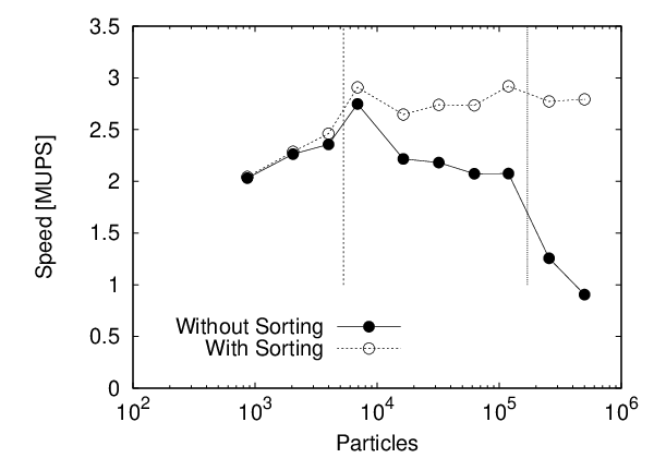
A comparison between the computational speed with and without sorting is shown in Fig. 8. The simulations were performed on a Xeon 2.93 GHz machine with 256 KB for an L2 cache and 8 MB for an L3 cache. We performed the sorting every ten constructions of a pair list, which is typically every few hundred time steps, since the computational cost of sorting is not expensive but not negligible. To mimic a configuration after a very long time evolution without sorting, the indices of the particles were completely shuffled at the beginning of the simulation, that is, the labels of the particles were exchanged randomly while keeping their positions and momenta. The computational speed is measured in the unit of MUPS (millions update per second), which is unity when one million particles are updated in one second. As the number of particles increased, the computational efficiency was greatly improved by sorting. The stepwise behavior of the data without sorting reflected the cache hierarchy. Since the system is three dimensional, amount of memory required to store information of one particle is 48 bytes. Therefore, L2 cache (256) KB corresponds to 256 KB/48 bytes and L3 cache (8MB) corresponds 8 MB/48 bytes . When the number of particles was smaller than , the difference in speed between the data with and without sorting was moderate. While the number of particles was larger than , we found that the efficiency was improved by 30 to 40% by sorting. When the number of particles was larger than , the computational speed without sorting became much lower than that with sorting. We found that the effect of the sorting in efficiency was about a factor of 3 in the case of particles.

3.4 Software Pipelining

The elimination of the conditional branch can be inefficient in some types of CPU architectures such as Intel or AMD,
since the cost of the conditional branch is not expensive. In such CPU architectures, software pipelining is
effective in improving the computational speed.
Recent CPUs can handle four or more floating-point operations simultaneously if they are independent.
The force calculation of one pair, however, consists of a sequence of instructions that are dependent on each other.
Therefore, CPU sometimes has to wait for the previous instruction to be completed, which decreases the computational speed.
Software pipelining is a technique to reduce such dependencies between instructions
in order to increase the efficiency of the calculation.
The purpose of the software pipening is increasing a number of instructions which can be
executed simultaneously, and consequently, increasing the instruction throughputs
in a hardware pipepine.
While the software-pipelining technique is often used in combination with loop unrolling,
the simple loop unrolling can cause a shortage of registers
leading to access to the memory which can be expensive.
The main idea of software pipelining is to calculate independent parts of the force calculation simultaneously by shifting the order of the instructions.
The calculation of force can be broken into the following five stages;
DIS calculate distance between two particles.
SQR calculate the square of the distance.
CMP compare the distance and the cutoff length.
CFD calculate the force using the distance.
UMP update the momentum of the particle.
The schematic image of the software pipelining is shown in Fig. 9.
The number after a stage denotes the index of the pair (the value of the loop counter), e. g.,
DIS1 denotes the calculation of the distance of the first particle pair.
Figure 9 (a) denotes the calculation without software pipelining.
Suppose the distances between third and fifth pairs are longer than the cutoff length.
Then the calculation of the force and the update the momentum are unnecessary.
We refer this to NOP (no operation).
All calculations are performed sequentially. For instance, SQR1 is performed after
DIS1 is completed, CMP1 is performed after SQR1 is completed, and so on.
Figure 9 (a) denotes the calculation with software pipelining.
The order of the calculations are shifted so that the number of independent calculations
are increased. For instance, DIS4, SQR3, and UMP1 can be performed simultaneously
since there are no dependencies between them (see the column where the value of the loop counter is three).
Increase of independent instructions increases the efficiency of the hardware pipeline,
and consequently, impoves the computational speed
The pseudo code corresponding to Fig. 9 is shown in Algorithm 8.
As far as we know in our experience, the software pipelining without loop unrolling described
here is the best choice for recent architecture such as Intel Xeon processors.
4 Parallelization
4.1 Parallelization Scheme
Since the size of the system or computational steps are limited on the single process job, parallel computation is required in order to simulate large systems or long time steps. Parallel computation is executed on a parallel environment such as a supercomputer. A total system of a supercomputer has hierarchic structure, i.e., a total system consists of nodes, a node consists of CPUs, a CPU consists of cores (see Fig. 10). One or two processes is usually executed on a single core, and a set of processes work concertedly on the same task.

There has been considerable effort devoted to the parallelization of MD simulations. The parallel algorithms used for MD can be classified into three strategies, domain decomposition, particle decomposition, and force decomposition [12]. In domain decomposition (also called spatial decomposition) the simulation box is subdivided into small domains, and each domain is assigned to each process. In particle decomposition, the computational workload is divided and distributed on the basis of the particles. Different processes have different particles. In force decomposition the computational workload is divided and distributed on the basis of the force calculation. Consider a matrix that denotes the force between - and -particles. Force decomposition is based on the block decomposition of this force matrix. Each block of the force matrix is assigned to each process. Generally, domain decomposition is suitable for systems with short-range interactions and simulations with a large number of particles [26, 27], and force decomposition is suitable for systems with long-range interactions such as electrostatic force and simulations with a large number of steps. In the present paper, we adopt a simple domain decomposition method for parallelization, i.e., we divide a system into small cubes of identical size. We use a Message Passing Interface (MPI) for all communication. To perform the computation, three types of communication are necessary: (i) exchanging particles that stray from the originally associated process, (ii) exchanging information of particles near boundaries to consider the cross-border interactions, and (iii) synchronization of the validity check of pair lists.
4.2 Exchanging Particles
Although all particles are initially in the domains to which they are placed, they tend to stray from their original domains as a simulation progresses. Therefore, each process should pass the migrated particles to an appropriate process at an appropriate time. There is no need for exchanging particles each step since it will not cause problems while migration distances are short. Therefore, migrated particles are exchanged simultaneously with a reconstruction of pair list.
4.3 Cross-Border Interactions

To calculate forces between particle pairs which are assigned to different processes, communication between neighboring processes is necessary. While a naive implementation involves communication in 26 directions since each process has 26 neighbors, the number of communications can be reduced to six by forwarding information of particles sent by other processes. Suppose a process is assigned the cuboidal domain , and , and the search length is denoted by , which is defined in Sec. 2.3. The procedures to send and receive positions of particles on the boundaries are as follows.
After the above six communications, exchanging positions of particles close to boundaries are completed including between diagonal processes. The details are illustrated in Fig. 11. Note that the simple implementation of the communication may cause deadlock which is a situation that two or more processes will wait responce forever. Suppose there are two processes, A and B. If A tries to send a message to B, and B also tries to send to A with MPI blocking communications, then the communication will not be completed. Similarly, suppose there are three processes, A, B, and C. If the communication path are A B, B C, and C A, then the system is getting into a deadlock. In the domain decomposition parallelism with periodic boundary condition, it is possible that a deadlock occurs. There are several techniques to avoid this problem, such as reversing the order of sending and receiving and using nonblocking operations. A simple way to avoid such a deadlock problem is to use the MPI_Sendrecv function. This function does not cause deadlock for closed-path communications. The pseudocode using MPI_Sendrecv is shown in Algorithm 9. and denote the direction that the process should send to or recieve from. There are six directions to complete the communication. The number of particles to be sent in each direction is fixed until the expiration of a pair list. Suppose is a number of particles to send. Then the number of data sent is , since only coordinates are required to calculate forces. The message tag denoted by , which is an arbitrary non-negative integer but it should be the same for sender and receiver.
4.4 Synchronization of pair list Constructions
Each process maintains its own pair list and has to reconstruct it when it expires. If each process checks the validity of the pair list and reconstructs it independently, since it causes idle time, and the calculation effiency dicreases. To solve this problem, we synchronize the validity check of pair lists for all processes, that is, we reconstruct all the pair lists even when one of the pair lists has expired. While this reduces the average lifetime of the pair lists, the overall speed of the simulation is greatly improved since the idle time is eliminated (see Fig. 12). This synchronization process can be implemented with MPI_Allreduce, which is a global-reduction function of the MPI. Note that the global synchronization of pair lists can have a serious effect on the parallel efficiency when a system is highly inhomogeneous such as a system involving phase transitions or a heat-conducting system. In such cases, further advanced treatment that manages pair lists locally at each location of grid would be required.

4.5 Results of Benchmark Simulations
To measure the efficiency of the developed code, we perform benchmark simulations on two different parallel computers located at the different facilities, which are NIFS and ISSP. The details of the computers are listed in Table 1. In the actual analysis we used the so-called week scaling analysis, which is the dependence of the execution time in terms of node number under the condition of the number of particle per process keeping constant. The conditions for the benchmark simulations are as follows. Note that, all quantities are normarized by well depth and atomic diameter of the Lennards-Jones potential defined in Sec. 2.1.
- •
System size: for each process.
- •
Number of particles: 500,000 for each process (number density is 0.5).
- •
Initial condition: Face-centered-cubic lattice.
- •
Boundary condition: Periodic for all axes.
- •
Integration scheme: Second-order symplectic integration.
- •
Time step: 0.001.
- •
Cutoff length: 2.5.
- •
Search length: 2.8.
- •
Cutoff scheme: Add constant and quadratic terms to potential as shown in Eq. (2).
- •
Initial velocity: The absolute value of the velocities of all particles are set to be 0.9 and the directions of the velocities are given randomly.
- •
After 150 steps, we measure the calculation (elapsed) time for the next 1000 steps.
When a system with particles is simulated for steps in seconds, then the number of MUPS is given by . At NIFS, we placed cubes at each node, and assigned one cube to each process (see Fig. 13), since each node has 32 cores, and we placed 64 processes on each node utilizing simultaneous multithreading (SMT). At ISSP, we placed cubes at each node, and assigned one cube to each process, since one node consists of two CPUs (8 cores) at ISSP.
| Facility | Name | CPU | Cores | Processes | Memory |
|---|---|---|---|---|---|
| NIFS | HITACHI SR16000/J2 | IBM POWER6 (4.7 GHz) | 32 | 64 (*) | 128GB |
| ISSP | SGI Altix ICE 8400EX | Intel Xeon X5570 (2.93 GHz) | 8 | 4 or 8 (**) | 24GB |

The results obtained at NIFS and ISSP are summarized in Table 2 and Table 3, respectively. Both results are shown in Fig. 14. While the elapsed time of the 2-node calculation at NIFS is 302.6 s, that of the 128-node calculation is 412.7 s. Similarly, while the elapsed time of the single node calculation at ISSP is 183.13 s, that of the 1024-node calculation is 272.478 s. Since we perform weak scaling, the elapsed time should be independent of the number of processes provided the computations are perfectly parallelized. Therefore, the increase in elapsed time of the calculation with larger nodes is regarded as being due to the parallel overhead.
| Nodes | Processes | Particles | Elapsed Time [s] | Speed [MUPS] | Efficiency |
|---|---|---|---|---|---|
| 2 | 128 | 64,000,000 | 302.623 | 211.484 | 1.00 |
| 4 | 256 | 128,000,000 | 305.469 | 419.027 | 0.99 |
| 8 | 512 | 256,000,000 | 309.688 | 826.638 | 0.98 |
| 16 | 1024 | 512,000,000 | 325.744 | 1571.79 | 0.93 |
| 32 | 2048 | 1,024,000,000 | 333.140 | 3073.78 | 0.91 |
| 64 | 4096 | 2,048,000,000 | 385.765 | 5308.93 | 0.78 |
| 128 | 8192 | 4,096,000,000 | 412.717 | 9924.48 | 0.73 |
| Nodes | Processes | Particles | Elapsed Time [s] | Speed [MUPS] | Efficiency |
|---|---|---|---|---|---|
| 1 | 2000000 | 183.13 | 10.9212 | 1.00 | |
| 2 | 8000000 | 186.296 | 42.9424 | 0.98 | |
| 4 | 16000000 | 187.751 | 85.2194 | 0.98 | |
| 8 | 32000000 | 190.325 | 168.133 | 0.96 | |
| 16 | 64000000 | 194.932 | 328.32 | 0.94 | |
| 32 | 128000000 | 203.838 | 627.95 | 0.90 | |
| 64 | 256000000 | 224.028 | 1142.71 | 0.82 | |
| 128 | 512000000 | 228.485 | 2240.84 | 0.80 | |
| 1024 | 4096000000 | 272.478 | 15032.4 | 0.66 |

5 Parallel Overhead
The benchmark results described in the previous section show that the parallelization efficiency decreases as a number of processes increases, while the ammount of communication in one step seems to be negligible compared with the computations. In the present section, we investigate the cause of the parallel overhead of our codes in order to identify the factor of the decrease in parallelization efficiency. All simulations presented here are performed under the same condition as that used for the benchmarks in Sec. 4.5.
5.1 Granularity
In parallel computing, the ratio of computation to communication is important. This ratio is called the granularity. Fine-grain parallelism refers to the situation that data are transferred frequently and computational tasks are relatively light compared with communication. Coarse-grained parallelism, on the other hand, refers to the situation that computational tasks are relatively heavy compared with communication. In general, a program having coarse granularity exhibits better performance for a large number of processes. Here, we estimate the granularity of our code. Although the interaction length is set to , each process has to send and receive information of particles whose distances from boundaries are less than , since we adopt the DUTC method and the search length is set to . Each process is assigned to a cube of length and the number density is set to . The communications are performed along the -, -, and -directions, and two communications are involved for each direction. The amount of transmitting data increases in order of the -, -, and - directions, since the received data of particles are forwarded. The position of each particle is expressed by three double-precision floating-point numbers, requiring bytes. The amount of communication along -axis is larger than that along -axis, since the information of particles recieved along -axis are transfered to -axis (see Fig. 11). The number of particles transmitted along the -axis is . Therefore, 336 KB are transmitted along the -axis. Similarly, = 355 KB of data are transmitted along the -axis and 375 KB of data are transmitted along the -axis. Since inner-node communication is performed on shared memory and should be sufficiently faster than internode communication, we only consider the internode communication. Each node at NIFS has cubes, and therefore, 16 processes involve internode communication. The largest amount of communication is along the -axis, which is about 375 KB 6 MB. The bandwidth between each node at NIFS is about 5 GB/s. The total amount of internode communication is at most 36 MB, and therefore, the time spent on communication will be about 7.2 ms for each step. The computational time without communication is about 0.3 s, which is 500 times longer than the estimated communication time. This implies that this code has coarse-grained parallelism and should be less affected by increasing the number of processes. The benchmark results, however, show a significant decrease in parallel efficiency for large-scale runs.
We have also investigated the communication set up time at Kyushu University. The supercomputer at Kyushu University is HITACHI SR16000/J2 which is same as that at NIFS. But it is 42 nodes while NIFS has 128 nodes. We observed the communication set up time for MPI_Barrier and MPI_Allreduce over full of nodes, and found that the set up times are at most 50 us and 130 us, respectively. Therefore, communication cannot be a main factor of the parallel overhead.
| Nodes | Total [s] | Force [s] | pair list [s] | Communication [s] |
|---|---|---|---|---|
| 2 | 304.609 | 217.403 | 38.26566 | 12.54 |
| 128 | 404.335 | 217.733 | 41.85143 | 14.39 |
| Nodes | Total [s] | Force [s] | pair list [s] | Communication [s] |
|---|---|---|---|---|
| 1 | 180.945 | 144.92 | 14.388425 | 4.12 |
| 256 | 228.614 | 144.638 | 16.299467 | 7.92 |

5.2 Lifetime of Pair Lists
Since we perform weak scaling analysis, the size of the system increases as the number of nodes increases. This can decrease the lifetime of pair lists, since the maximum speed of the particles increases in a larger system and faster particles reduce the lifetime of pair lists [28]. The construction of a pair list takes much longer time than the force comutation takes, and therefore, the simulation run time is strongly affected if the number of pair lists being constructed increases. This increases the simulation run time even if the simulation is perfectly parallelized, and therefore, it is inappropriate to regard this cost as the parallelization cost. Therefore, we investigate the system-size dependence on the time required for construction of pair lists. At NIFS, the pair list was reconstructed 20 times for the 2-node run while it was reconstructed 21 times for the 128-node run. The average life time is 51.2 steps for 2-node and 53.8 steps for 128-node caluclations. Therefore, the computational cost to construct pair lists increases for larger number of nodes, but the difference is small. The breakdowns of the computational time for the smallest and the largest runs are listed in Table 4 and 5 and are also shown in Fig. 15. The additional cost of the pair list construction at NIFS is only 4 [s] which cannot explain the parallel overhead, which is over 100 [s]. Therefore, the lifetime of pair lists is not the main factor causing the reduced parallel performance.
5.3 Communication Management
Each simulation involves two types of communication at each step. One is point-to-point communication for sending and receiving data of particles, the other is collective communication for the synchronization of pair lists. The point-to-point communication is implemented in a simple way, that is, all processes send data in one direction and receive data from the opposite direction. All processes send and receive data simultaneously in the same direction using MPI_Sendrecv (see Fig. 16 (a)). While the simple implementation of the communication may cause deadlock for the system with THE periodic boundary condition, the function MPI_Sendrecv avoid the deadlock implicitly by reordering of communication, which may cause some overhead in parallel efficiency for a large number of processes. Therefore, we examine different ways of communication which avoid the deadlock explicitly in order to investigate whether the communication management by MPI_Sendrecv is the factor of the parallel overhead. Here we performed three methods. The first method, referred to as ‘Oneway’, is the simple implementation described in Sec. 4.3. The second method, referred to as ‘Two-step Oneway’, involves communications in 2 stages (see Fig. 16 (b)). All processes are classified into two groups, even and odd. In the first of the two stages, even processes send data and odd processes receive data. In the second stage, data are transmitted in the reverse direction. The communications are implemented by the blocking functions MPI_Send and MPI_Recv. The third method, referred to as ‘Pairwise’, arranges the order of communication explicitly. All processes are classified into two groups, even and odd, similarly to in the previous method. When the even processes exchange data with their right neighbors, the other processes exchange data with their left neighbors, and vice versa (see Fig. 16 (c)). The communications are implemented by MPI_Sendrecv. Note that, the behavior of ‘Pairwise’ at ISSP is not monotonic, i.e., the data of 128-node run is much faster than those of 8-, 16-, 32-, and 64-node runs. This may be due to the network topology at ISSP which is hypercube, however, the details should be investigated later.

A comparison of benchmark test for above the three methods is shown in Fig. 17. Figure 17 (a) shows the results at NIFS. The results of Pairwise only slightly differ from those of Oneway. While the results of Two-step Oneway show similar performance up to 32 nodes, those for larger nodes are significantly slower than the other methods. Figure 17 (b) shows the results at ISSP. There are major differences between the performances of the three methods even though the amounts of communication are identical, and Two-step Oneway considerably slower than the other methods. The reason why Two-step Oneway is the slowest method in both cases may be that double threads are executed by separating the sending and receiving processes instead of using MPI_Sendrecv. While it is unclear why the results of the three methods are almost the same for the largest number of nodes at ISSP, we can conclude that the overhead of communications strongly depends on the hardware environment. Considering the above results at NIFS and ISSP, the simple Oneway scheme is found to be less affected by the architecture of parallel machine and consistently has relatively good performance.


5.4 Synchronicity Problem
Parallel programs adopting the single program multiple data (SPMD) model usually require synchronicity, and the parallel MD described here is one such example. The slowest process determines the overall performance, since other processes must wait for the slowest process owing to the synchronization. Therefore, the parallel efficiency is strongly affected by the fluctuation of the computation time of each process. One of the factors causing the fluctuation is load imbalance. Load imbalance refers to the inhomogeneity of workload among processes. Unequally assigned tasks cause the fluctuation of the computational time of each step and they decrease the parallel efficiency. The workload of parallel MD mainly depends on the number of interacting pairs in each process. To clarify this problem quantitatively, the number of interacting pairs is counted at the final state of the 128-node run. The parallel efficiency is determined by the slowest process which should be with the largest number of interacting pairs.
In our calculation, we found that the largest and the smallest number of pairs were and , respectively. The difference is about , which cannot be responsible for the reduction in parallel efficiency. Note that this small fluctuation originates from the fact that the initial condition is homogeneous. The load imbalance can be serious for inhomogeneous systems such as systems involving phase transitions. However, our benchmark results show that the parallel efficiency decreases as the number of processes increases, even for a homogeneous system with a uniform workload for each process. Therefore, we assumed that there are other factors that affect the parallel efficiency.
Next, we investigate the fluctuation of the computational time of force for each process. Suppose is the computational time spent for force calculation of -th process at -th step. The average of the force calculation at -th step is defined as
| (7) |
with the number of processes . The time evolutions of at NIFS and ISSP are shown in Fig. 18. The data of the smallest and the largest runs are presented. Note that, we observe the time spent only for force calculation which dose not involve communication. We found that the computational time for force show almost same values and independent of the number of nodes. However, the compuational time for each step itself might fluctuate, which cause the one of candidate of reduction of parallel efficiency. Therefore, we focus on the calculation time of force for each step. To investigate the fluctuation of the computational time for each step, we define the relative difference as
| (8) |
where is the maximum time, and is the minimum time spent on the force calculation among all processes at th step [29]. denotes the difference between the times spent on the slowest and fastest processes normalized by the average time at th step. The time evolutions of the average and relative difference for force calculations at NIFS are shown in Fig. 19 (a). While the average times for force calculations are identical for 2- and 128-node runs, the relative differences of the large run are significantly larger than those of the small run. The relative difference of the large run sometimes fluctuates by 100% ( becomes 1.0), which implies that the computational time is doubled at the step. The same plots for ISSP are shown in Fig. 19 (b). Similar phenomena are observed, although the relative differences of the large run are at most 40%. The relative differences of the small run at ISSP are almost zero, since the run has only four processes, which is the reason why the fluctuation is relatively small.
From the above, we can conclude that the main factor degrading the parallel efficiency is the fluctuation of the computational time at each step. Although the average time varies only slightly, the fluctuation of the computational time between processes increases as the number of processes increases. Then the delays of the slowest process accumulate as the overhead. There are several possible factors causing this fluctuation. One possible source is noise from an operating system (OS). An OS has several background processes called daemons, which interfere with the user execution time and decreases its efficiency [30]. This noise from OS is referred to as OS jitter or OS detour. Interruptions by an operating system occur randomly, and they cause the fluctuation of the execution time of each process. Not only interruptions themselves, but also side effects caused by the interruptions, such as pollution of the CPU cache, are also a source of noise.


6 Summary and Further Issues
We have developed an MD code that is not only suitable for massively parallel processors but also exhibits good single-processor performance for IBM Power and Intel Xeon architectures. Most of all algorithms presented in this paper can be applied to other particle systems with short-range interactions including many-body interactions. There are three levels of optimization. At the highest level, we attempt to reduce the computational cost by developing or choosing appropriate algorithms such as the bookkeeping method. Next, we have to manage memory access. All data required by cores should be in the cache so that the cores make the best use of its computational power. Finally, we have to perform architecture-dependent tuning, since the development paradigms are considerably different between different CPUs.
MD is suitable for MPP-type simulations since the computation-communication ratio is generally small. However, we have observed a significant degradation in parallel efficiency despite the use of conditions under which the communication cost should be negligible. We have found that the fluctuation of the execution time of processes reduces the parallel efficiency. The fluctuations become serious when the number of process becomes over one thousand. The OS jitter, which is the interference by the operating system, can be a source of the fluctuation. There are many attempts to handle the OS jitter, but it is difficult to be settled by user programs. One possibility is to adopt hybrid parallelization, i.e., use OpenMP for inner-node communications and use MPI for internode communications. Hybrid parallelization not only reduces the number of total MPI processes, but also averages out the fluctuations which can improve the parallel efficiency. Note that the affect due to the OS jitter is generally order of nanoseconds or shorter, and the time required to perform one step of MD simulations is order of millisecond. Therefore, there may be other sources of noise, such as translation lookaside buffer (TLB) miss. TLB is a kind of cache, which translate the address from virtual to real [31]. While it makes computation faster, it takes long time to fetch the data if the required address is not cached in the buffer. The translation tables are somtimes swapped out into other storage such as hard-disk, then the penalty of TLB miss can be expensive. Investigation of the source of the fluctuation in execution time is one of the further issues.
In this paper, the load imbalance problem is not considered. Load balancing is important for parallelization with a huge number of processes since the fluctuation of the timing of each process greatly degrades the parallel efficiency as shown in Sec. 5.4. There are two approaches to load balancing, one is based on force decomposition and the other is based on domain decomposition. The load balancing in NAMD (Not Another Molecular Dynamics program) [7] is essentially achieved by the force decomposition, while NAMD adopts a hybrid strategy of parallelization. The processes of NAMD are under the control of a dynamic load balancer. The simulation box is divided into subdomains (called patches), and the total computational task is divided into subtasks (called compute objects). The load balancer measures the load on each process and reassigns compute objects to processors if necessary. GROMACS (Groningen Machine for Chemical Simulations) [8] adopts a domain-decomposition-based strategy for load balancing, that is, it changes the volume of domains assigned to processors to improve the load balance. The simulation box is divided into staggered grids whose volume are different. A load balancer changes the volume of each grid by moving the boundaries of cells to reduce load imbalance. There is also a method of non-box-type space decomposition that utilizes the Voronoi construction. Reference points are placed in a simulation box and each Voronoi cell is assigned to a process. Load balancing is performed by changing the positions of the reference points [32, 33]. Generally speaking, force-decomposition-based load balancing is a better choice if a system contains long-range interactions such as electrostatic force, and domain-decomposition-based load balancing is better for a system with short-range interactions. However, the choice strongly depends on the phenomenon to be simulated, and therefore, both strategies or some hybrid of them should be considered.
The source codes used in this paper has been published online [34]. We hope that the present paper and our source codes will help researchers to develop their own parallel MD codes that can utilize the computational power of petaflop, and eventually exaflop machines.
Acknowledgements
The authors would like to thank Y. Kanada, S. Takagi, and T. Boku for fruitful discussions. Some parts of the implementation techniques are owing to N. Soda and M. Itakura. HW thanks M. Isobe for useful information of past studies. This work was supported by KAUST GRP (KUK-I1-005-04), Grants-in-Aid for Scientific Research (Contracts No. 19740235), and the NIFS Collaboration Research program (NIFS10KTBS006). The computations were carried out using the facilities of National Institute for Fusion Science; the Information Technology Center, the University of Tokyo; the Supercomputer Center, Institute for Solid State Physics, University of Tokyo; and the Research Institute for Information Technology, Kyushu University.
References
- [1] B. J. Alder and T. E. Wainwright, J. Chem. Phys. 27 (1957), 1208.
- [2] A. Rahman, \PR136,1964,405.
- [3] M. P. Allen and D. J. Tildesley, Computer Simulation of Liquids, (Clarendon Press, Oxford 1987).
- [4] D. Frenkel and B. Smit, Understanding Molecular Simulation – From Algorithms to Applications, (Academic Press, NewYork, 2001)
- [5] D. Rapaport, The art of molecular dynamics simulation, (Cambridge University Press, 2004).
- [6] W. G. Hoover, Molecular Dynamics, Lecture Notes in Physics 258 (Springer-Verlag, Berlin, 1986).
- [7] L. Kalé, R. Skeel, M. Bhandarkar, R. Brunner, A. Gursoy, N. Krawetz, J. Phillips, A. Shinozaki, K. Varadarajan, and K. Schulten, J. Comput. Phys. 151, (1999), 283.
- [8] B. Hess, C. Kutzner, D. van der Spoel, and E. Lindahl, J. Chem. Theory Comput. 4 (2008) 435.
- [9] R. Car and M. Parrinello, \PRL55,1985,2471.
- [10]
http://www.top500.org/ - [11]
http://www.nsc.riken.jp/ - [12] S. Plimpton, J. Comput. Phys. 117 (1995), 117.
- [13] T. C. Germann and K. Kadau, \IJMPC19,2008,1315.
- [14] B. L. Holian, A. F. Voter, N. J. Wagner, R. J. Ravelo, and S. P. Chen, \PRA43,1991,2655.
- [15] D. M. Beazley and P. S. Lomdahl, Parallel Comput. 20 (1994), 173.
- [16] S. D. Stoddard and J. Ford, \PRA8,1973,1504.
- [17] B. Quentrec and C. Brot, J. Comput. Phys. 13 (1975), 430.
- [18] R. W. Hockney and J. W. Eastwood, Computer Simulation Using Particles (McGraw-Hill, New York, 1981).
- [19] W. Form, N, Ito, and G. A. Kohring, \IJMPC4,1993,1085.
- [20] D. E. Knuth, The Art of Computer Programming (Addison–Wesley, Reading, MA, 1973).
- [21] G. S. Grest and B. Dünweg, Comput. Phys. Commun. 55 (1989) 269.
- [22] K. Kadau, T. C. Germann, and P. S. Lomdahl, \IJMPC17,2006,1755.
- [23] L. Verlet, \PR195,1967,98.
- [24] M. Isobe, \IJMPC10,1999,1281.
- [25] S. Meloni, M. Rosati, and L. Colombo, J. Chem. Phys. 126 (2007), 121102.
- [26] R. Hayashi, K. Tanaka, S. Horiguchi, and Y. Hiwatari, Parallel Processing Letters, 15, (2005) 481.
- [27] D.M. Beazley, P.S. Lomdahl, N.G. Jensen, R. Giles, and P. Tamayo, Parallel Algorithms for Short-Range Molecular Dynamics., World Scientific’s Annual Reviews in Computational Physics, 3, (1995) 119.
- [28] In equilibrium, a distribution for the velocity obeys the Maxwell–Boltzmann type. While there can be an infinitely fast particle in an infinite-size system, the exectation value of the maximum velocity is finite in the finite-size system and the value increases as the system size increases.
- [29] We investigated the difference between the maximum and the minimum time spent for force calculation amoung processes instead of the standard deviation, since the slowest process determine the global speed of the calculation and the quantity observed in the present manuscript is directly associated with the parallel overhead. It is also worth to be noted that the probability distribution function of is not the Gaussian type. Therefore, the standard deviation is not an appropriate index to characterize the fluctuation of the calculation time.
- [30] P. Beckman, K. Iskra, K. Yoshii, and S. Coghlan, ACM SIGOPS Operating Systems Review 40, (2006) 29.
- [31] A. S. Tanenbaum, Modern Operating Systems, (Prentice Hall, 2001).
- [32] H. Yahagi, M. Mori, and Y. Yoshii, ApJS, 124 (1999), 1.
- [33] R. Koradi, M. Billeter, and P. Guinter, Comput. Phys. Comm. 124 (2000), 139.
- [34]
http://mdacp.sourceforge.net/