Real-time Visual Tracking Using Sparse Representation

From a Bayesian perspective, the tracking problem is to calculate the posterior probability $p(\mathbf{s}_{k}|{\mathbf{y}}_{k})$ of state $\mathbf{s}_{k}$ at time $k$, where ${\mathbf{y}}_{k}$ is the observed measurement at time $k$ [13]. In principle, the posterior PDF is obtained recursively via two stages: prediction and update. The prediction stage involves the calculation of prior PDF:

In the update stage, the prior is updated using Bayes’ rule

The recurrence relations (1) and (2) form the basis for the optimal Bayesian solution. Nonetheless, the solution of above problem can not be analytically solved without further simplification or approximation. Particle Filter (PF) is a Bayesian sequential importance sampling technique for estimating the posterior distribution $p(\mathbf{s}_{k}|{\mathbf{y}}_{k})$. By introducing the so-called importance sampling distribution [8]:

the posterior density is estimated by a weighted approximation,

Here

For the sake of convenience, $q(\cdot)$ is commonly formed as

Therefore, (5) is simplified into

The posterior then could be updated only depending on its previous value and observation likelihood $p(\mathbf{s}_{k}|\mathbf{s}_{k-1}^{i})$. Plus, in order to reducing the effect of particle degeneracy [8], a resampling scheme is usually implemented as

where the set $\{\mathbf{s}_{k}^{i*}\}_{i=1}^{N_{s}}$ is the particles after re-sampling.

Like the $\ell_{1}$ tracker, both RTCST and RTCST-B trackers use PF framework. However, they differ in how to seek a sparse representation which consequently lead to different observation likelihood $p(\mathbf{s}_{k}|\mathbf{s}_{k-1}^{i})$ estimtation.

The underlying conception behind SRC is that in many circumstances, an observation belonging to a certain class lies in the subspace that is spanned by the samples belong to this class, and the linear representation is assumed to be sparse. Hence, reconstructing the sparse coefficients associated with the representation is crucial to identify the observation. The coefficients recovery could be accomplished by solving a relaxed version of (13)

where ${\mathbf{x}}\in\mathbb{R}^{n}$ is the coefficient vector of interest; $A=[\mathbf{a}_{1},$ $\mathbf{a}_{2},\dots,$ $\mathbf{a}_{n}]\in\mathbb{R}^{d\times n}$ is sometimes dubbed as dictionary and composed of pre-obtained pattern samples $a_{i}\in\mathbb{R}^{d}~\forall i$; and ${\mathbf{y}}\in\mathbb{R}^{d}$ is the query/test observation. $\varepsilon$ is error tolerance. Then, the class identity $l({\mathbf{y}})$ is retrieved as

where $r_{j}({\mathbf{y}})\doteq\|{\mathbf{y}}-A\delta_{j}({\mathbf{x}})\|_{2}$ is the reconstruction residual associated with class $i$, $C$ is the number of classes and the function $\delta_{j}({\mathbf{x}})$ sets all the coefficients of ${\mathbf{x}}$ to $0$ except those corresponding to $j$th class [17].

Given a target template set $T=[{\mathbf{t}}_{1},\cdots,{\mathbf{t}}_{N_{t}}]\in\mathbb{R}^{d_{0}\times N_{t}}$ and a noise template set $E=[I,\;-I]\in\mathbb{R}^{d_{0}\times 2d_{0}}$, the $\ell_{1}$ tracker adopts a positive-restricted version of (14) for recovering the sparse coefficients ${\mathbf{x}}$, i.e.,

Here $A\doteq[T,E]\in\mathbb{R}^{d_{0}\times(N_{t}+2d_{0})}$ is the combination of target templates and noise templates while ${\mathbf{x}}\doteq[{\mathbf{x}}_{t}^{\!\top},~{\mathbf{x}}_{e}^{\!\top}]^{\!\top}\in\mathbb{R}^{N_{t}+2d_{0}}$ denotes the associated target coefficients and noise coefficients. Note that $N_{t}$ denotes the number of target templates and $d_{0}$ is the original dimensionality of feature space which equals to the pixel number of the initial target. The $\ell_{1}$ tracker tracks the target by integrating (11) and a template-update strategy into the PF framework. Algorithm 1 illustrates the tracking procedure. In addition, there is a heuristic approach for updating the target templates and their weights in the $\ell_{1}$ tracker. Refer to [1] for more details.

CS states that a $\eta$-sparse¹¹ 1 a signal ${\mathbf{x}}$ is said $\eta$-sparse if there are at most $\eta$ nonzero entries in ${\mathbf{x}}$. signal ${\mathbf{x}}\in\mathbb{R}^{n}$ can be exactly recovered with overwhelming probability via few measurements

Intuitively, one would achieve ${\mathbf{x}}$ via

where $\Phi\in\mathbb{R}^{m\times n}$ is the measurement matrix, of which rows are the measurement vectors $\Phi_{i}$ and ${\mathbf{y}}=(y_{1},\dots,y_{m})^{T}$. $\|{\mathbf{x}}\|_{0}$ is the number of non-zero elements of ${\mathbf{x}}$. Since (12) is NP-hard [22], it is commonly relaxed to

which can be casted into a linear programming problem.

As regards CS-based pattern recognition, to deal with noise, one could alternatively solve a Second Order Cone Program:

where $\varepsilon$ is a pre specified tolerance.

The biggest problem of $\ell_{1}$ tracking is the extremely high dimensionality of the feature space, which leads to heavy computation. More precisely, suppose that the cropped image of observation is $I\in\mathbb{R}^{h\times w}$, the dimensionality $d_{0}=h\cdot w$ is typically in the order of $10^{3}\sim 10^{5}$, which prevents tracking from real-time.

Fortunately, in the context of compressed sensing (ignoring the non-negativity constraint on ${\mathbf{x}}$ for now), it is well known that if the measurement matrix $\Phi$ has Restricted Isometry Property (RIP) [19], then a sparse signal ${\mathbf{x}}$ can be recovered from

A typical choice of such measurement matrix is random gaussian matrix

Besides random projection, there are other means that guarantee RIP. Shi et al. [23] proposed a hash kernel to deal with the issue of computational efficiency. Let $h_{s}(j,d)$ denotes a hash function (i.e., the hash kernel) $h_{s}:\mathbb{N}\to\{1,\dots,d\}$ drawn from a distribution of pairwise independent hash functions, where $s\in\{1,\dots,S\}$ is the seed. Different seed gives different hash function. Given $h_{s}(j,d)$, the hash matrix $H$ is defined as

Obviously, $H_{ij}\in\{0,\pm 1\}$. The hash kernel generates hash matrices more efficiently than conventional random matrices while maintains the similar random characteristics, which implies good RIP.

In this work, the dimensionality of feature space is reduced by matrix $\Phi\in\mathbb{R}^{d\times d_{0}}$ (which could be either random matrix $R$ or hash matrix $H$) from $d_{0}$ to $d$ where $d\ll d_{0}$. This significantly speeds up solving equation (14), for its complexity depends on $d$ polynomially.

Besides the dimension reduction methods and OMP, modifications to the original $\ell_{1}$ tracker are proposed in this section to achieve a even higher tracking accuracy.

In a nutshell, for each observation, we utilize Algorithm 2 to recover the coefficient vector ${\mathbf{x}}$ by solving the problem

where ${\mathbf{x}}=[{\mathbf{x}}_{t},~{\mathbf{x}}_{e}]$, $A=[T,~E]$. The residual is then obtained by

Finally the likelihood of this observation is updated as

The procedure of Real-Time Compressed Sensing Tracking algorithm is summarized in Algorithm 3. Our template update scheme is demonstrated in Algorithm 4. As can be seen, the proposed update scheme is much conciser than that in the $\ell_{1}$ tracker [1] thanks to the abandonment of template weight. The empirical performance of RTCST is verified in Section V.

A good CSBM should only constitute “pure” backgrounds and contain sufficiently large appearance variation, e.g., illumination changes. Ideally, we could simply select certain number of foreground-absent frames from video sequence to build a CSBM. However, the “pure” background is usually difficult to find and it is even harder to obtain the ones cover the main distribution of background appearance.

An intuitive way to obtain a clean background is replacing the foreground of one frame with a background patch cropped from another frame. More precisely, let $F\in\mathbb{R}^{h\times w}$ denote the frame based on which the background is retrieved, and $F^{\prime}\in\mathbb{R}^{h\times w}$ stand for the frame where the background patch is cropped, suppose that the foreground region in $F$ is $F(t:b,l:r)$⁴⁴ 4 In this paper, all the target or foreground is represented as a rectangle region, the patching operation could be described as

where $\Gamma$ is the retrieved background. An illustration of (29) is also available in Figure 3.

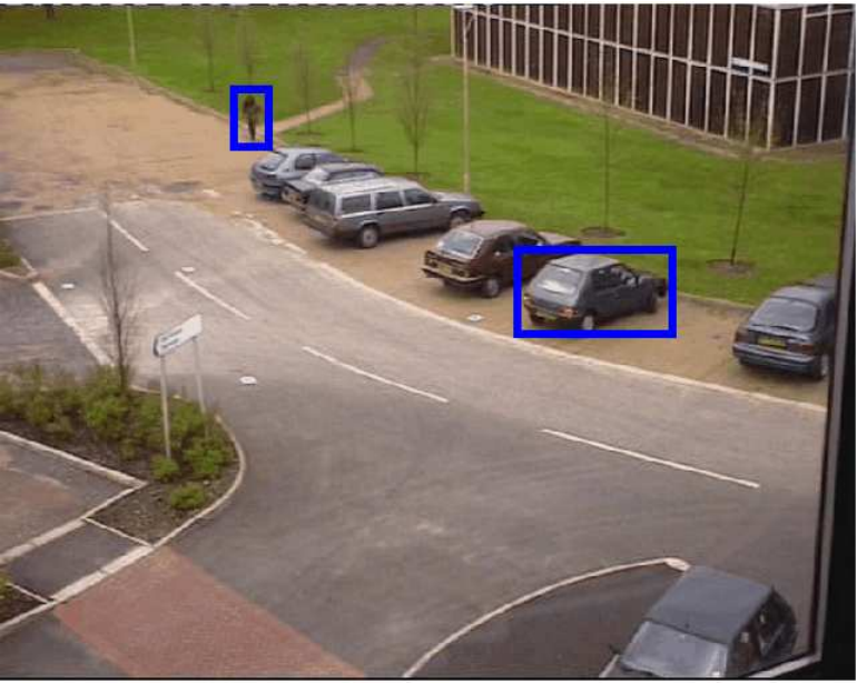
In practice, multiple foreground regions need to be mended for each “impure” background candidate. Furthermore, a selection approach should be conducted to form the optimal combination of the retrieved backgrounds over all the candidates. To achieve this goal, we first randomly capture $N^{\prime}>N_{b}$ frames from the concerned video sequence. Afterwards, every foreground region of the frames are located manually. The foreground is then replaced by a clean background region cropped from the nearest frame (in terms of frame index). Finally, a $k$-median clustering algorithm is carried out for selecting $N_{b}$ most comprehensive backgrounds.

It is nontrivial to notice that even some backgrounds are not perfectly retrieved, i.e., with minor foreground remains, CSBM can still work well considering that CS is robust to the noise in measurements [19].

We equip the RTCST with CSBM to build a novel visual tracker, a.k.a Real-Time CS-based Tracker with Background Model (RTCST-B). In RTCST-B, original noise templates are replaced by background templates which are generated from CSBM. In the context of PF tracking, given a observation position $\Xi$ with $d_{0}$ pixels and a CSBM $\mathbb{G}$ defined in (28), the background templates set $B$ is obtained by:

where function $\text{CV}(\cdot)$ is called crop-vectorize operation which first crops the region indicated by $\Xi$ from background $\Gamma_{i}$ and then vectorize it into $I_{i}\in\mathbb{R}^{d_{0}}$. Eventually, the optimization problem for RTCST-B writes:

where ${\mathbf{x}}$ is comprised of ${\mathbf{x}}_{t}$ and ${\mathbf{x}}_{b}$, i.e., the coefficient vectors for target and background, $A=[T,~B]\in\mathbb{R}^{d\times(N_{t}+N_{b})}$.

Despite the diverse optimization problem, the calculation for the likelihood remains the same as in (27). To understand this, let ${\mathbf{x}}_{t}$ and ${\mathbf{x}}_{b}$ denote the coefficients associated with target templates and background templates respectively, $p({\mathbf{y}}_{k}|{\mathbf{s}})=p({\mathbf{y}}_{k}|{\mathbf{x}}_{t})=\exp(-\lambda r)$ be the observation likelihood⁵⁵ 5 It is trivial to prove that the relationship between particle ${\mathbf{s}}$ and ${\mathbf{x}}_{t}$ is deterministic given a specific frame image, where $r$ is defined in (26), then we have:

with the assumption that ${\mathbf{x}}_{t}$ and ${\mathbf{x}}_{b}$ are deterministic by each other, i.e.,

or in other words, the solution of CS procedure is unique. [19].

In addition, the template update scheme should be changed slightly considering a new class is involved in. More precisely, target templates are updated only when

Finally, the positive constraint for ${\mathbf{x}}$ is removed in 31 because background subtraction implies minus coefficients for background templates. It is reasonable to not curb the coefficients in RTCST-B.

In summary, one just needs to impose following minor modifications on RTCST to transfer it into RTCST-B.

1. 1.

   Substitute the background templates for noise templates.

2. 2.

   Eliminate the positive constraint.

3. 3.

   Conduct the CV operation for each observation.

4. 4.

   Utilize the new SCI measurement.

Apparently, the diversity between RTCST and RTCST-B is not significant with respect to formulation. Nevertheless, the seemingly small change makes RTCST-B much more superior to its prototypes.

Compared with the $\ell_{1}$ tracker and RTCST, RTCST-B enjoys three main advantages which are described as follows.

To verify the proposed tracking algorithms, we design a series of experiments for examining the tracking algorithm in terms of accuracy, efficiency and robustness. The proffered algorithms are conducted on $10$ video sequences comparing with $\ell_{1}$ tracker, Kernel-Mean-Shift (KMS) tracker [14] and color-based PF tracker[13]. The details of selected video sequences are list in Table II. Note that we only conduct $\ell_{1}$ tracker on $5$ videos which are cubicle, dp, car11, pets2001_c1 and pets2004-2_p1 respectively. It is because for other videos, the convex optimization problem is too slow to be solved (above $5$ minutes per frame).

There are two alternative dimension-reduction manners for RTCST and RTCST-B, namely, random projection and hash matrix projection. In our experiments, both of them are performed with reduced dimension $25$, $50$ and $100$. As regards the particles’ number, we examine the proposed trackers with $100$ and $200$ particles and the numbers for PF tracker is $100$, $200$ and $500$. All the PF-based trackers are run for $20$ times except $\ell_{1}$ tracker which is merely conducted for $3$ times. We perform KMS tracker for only $1$ time considering it is a deterministic method. The average values and standard errors are reported in this section. The MS tracker, PF tracker and $\ell_{1}$ tracker are implemented in C++ while our CS-based trackers are implemented in Matlab. To compare the efficiency with the proposed algorithms, there is also a Matlab version of $\ell_{1}$ tracker. All the algorithms are run on a PC with $2.6G$Hz quad-core CPU and $4G$ memory (we only use one core of it). As to the software, we use Matlab $2009a$ and the linear programming solver is called from Mosek $6.0$[30].

It is important to emphasize that in our experiment, no trick is used for selecting the target region in the first frame. The initial target region is always the minimum rectangle $R=[l,r,t,b]$ which can cover the whole target⁶⁶ 6 Shadows are not taken into consideration., where $l$, $r$, $t$, and $b$ are the left, right, top and bottom boundaries’ coordinates (horizontal or vertical) respectively. This rigid rule is followed for eliminating the artificial factors in visual tracking and making the comparison unprejudiced.

A conventional choice of the manner to verify the tracking accuracy is tracking error. Specifically, given that the centroid of ground truth region is ${\mathbf{c}}_{g}$ while that of tracked region is ${\mathbf{c}}_{t}$, the tracking error $\rho$ is defined as

i.e., the euclidean distance between two centroids. However, if we take scale variation into consideration, $\rho$ is poor to verify tracker’s performance. Let’s see Figure 6(a) for a example. In the image, red rectangle indicates the ground truth for a moving car. The blue and gray rectangles, which are obtained by various tracking algorithms, share the identical centroid. By using tracking error, same performance is reported for both two trackers despite the obvious difference on tracking accuracy.

Inspired by the evaluation manner proposed for PASCAL data base[31], we propose a new tracking accuracy measurement which is termed Tracking Success Probability (TSP). To obtain the definition of TSP, firstly let’s suppose the bounding box of ground truth region is $R_{g}=[l_{g},r_{g},t_{g},b_{g}]$, and the one for tracked region is $R_{t}=[l_{t},r_{t},t_{t},b_{t}]$. We then design a function $a(R_{g},R_{t})\in[-1,1]$ to estimate the overlapping state between $R_{g}$ and $R_{t}$. Given two distance sets:

and a indicator function $s_{tg}$

then $a(R_{g},R_{t})$ writes⁷⁷ 7 Here, we suppose the origin of image is on the left-top corner.

It is easy to find that when two regions overlap each other, $a(R_{g},R_{t})$ is the ratio of the intersection area $R_{g\cap d}$ to the area $R^{*}$, which is the minimum region covering both $R_{g}$ and $R_{d}$. See Figure 6(b) for an instance. Finally, TSP is formulated as

where $\nu>0$ is a preset parameter reflects the worst scenario we could assure the target is located correctly. In our experiment, $\nu$ is the solution of

In other words, when the overlapped region is larger than $25\%$ part of region $R^{*}$, we are convinced (with the probability of $0.95$) that the tracking is successful.

Obviously, the larger the TSP is, the more confident we believe this tracking is successful. If we apply TSP to the tracking results shown in Figure 6(a), then the TSP of blue rectangle is $0.95$ which is significantly larger than that of the gray one (with TSP of $0.55$). The difference implies that TSP is capable to accommodate dynamic factors besides displacement. Another merit of TSP is the comparability over different video sequences thanks to its fixed value range i.e., $[0,1]$. Considering these advantages, in the current paper, all the empirical results are evaluated by TSP. As a reference, tracking error results are also available.

Firstly, we examine the tracking accuracy of our trackers comparing with the competitors. The average TSP for every experiment is shown in Table III. For each video sequence, the optimal accuracy is displayed in bold type.

References

- [1] X. Mei and H. Ling, “Robust visual tracking using minimization,” in Proc. IEEE Int. Conf. Comp. Vis., Kyoto, Japan, 2009, pp. 1436–1443.
- [2] T. F. Cootes, G. J. Edwards, and C. J. Taylor, “Active appearance models,” IEEE Trans. Pattern Anal. Mach. Intell., pp. 484–498, 1998.
- [3] D. Comaniciu, V. Ramesh, and P. Meer, “Kernel-based object tracking,” IEEE Trans. Pattern Anal. Mach. Intell., vol. 25, pp. 564–577, 2003.
- [4] A. Yilmaz and M. Shah, “Contour-based object tracking with occlusion handling in video acquired using mobile cameras,” IEEE Trans. Pattern Anal. Mach. Intell., vol. 26, pp. 1531–1536, 2004.
- [5] S. Avidan, “Support vector tracking,” IEEE Trans. Pattern Anal. Mach. Intell., pp. 184–191, 2001.
- [6] D. Serby and L. V. Gool, “Probabilistic object tracking using multiple features,” in Proc. IEEE Int. Conf. Patt. Recogn., 2004, pp. 184–187.
- [7] C. Shen, J. Kim, and H. Wang, “Generalized kernel-based visual tracking,” IEEE Trans. Circuits Syst. Video Technol., vol. 20, pp. 119–130, 2010.
- [8] A. Doucet, S. Godsill, and C. Andrieu, “On sequential monte carlo sampling methods for bayesian filtering,” Statistics and Computing, vol. 10, no. 3, pp. 197–208, 2000.
- [9] C. Shen, M. J. Brooks, and A. van den Hengel, “Fast global kernel density mode seeking: applications to localization and tracking,” IEEE Trans. Image Process., vol. 16, no. 5, pp. 1457–1469, 2007.
- [10] M. L. Cascia, S. Sclaroff, and V. Athitsos, “Fast, reliable head tracking under varying illumination: An approach based on registration of texture-mapped 3d models,” IEEE Trans. Pattern Anal. Mach. Intell., vol. 22, pp. 322–336, 2000.
- [11] K. Shafique and M. Shah, “A non-iterative greedy algorithm for multi-frame point correspondence,” in IEEE Trans. Pattern Anal. Mach. Intell., 2003, pp. 51–65.
- [12] O. Williams, A. Blake, and R. Cipolla, “Sparse bayesian learning for efficient visual tracking,” IEEE Trans. Pattern Anal. Mach. Intell., vol. 27, pp. 1292–1304, 2005.
- [13] M. S. Arulampalam, S. Maskell, and N. Gordon, “A tutorial on particle filters for online nonlinear/non-gaussian bayesian tracking,” IEEE Trans. Signal Process., vol. 50, pp. 174–188, 2002.
- [14] D. Comaniciu, V. Ramesh, and P. Meer, “Kernel-based object tracking,” IEEE Trans. Pattern Anal. Mach. Intell., vol. 25, pp. 564–575, 2003.
- [15] F. Porikli, O. Tuzel, and P. Meer, “Covariance tracking using model update based on lie algebra,” in Proc. IEEE Conf. Comp. Vis. Patt. Recogn., 2006, vol. 1, pp. 728–735.
- [16] S. Zhou, R. Chellappa, and B. Moghaddam, “Visual tracking and recognition using appearance-adaptive models in particle filters,” IEEE Trans. Image Process., vol. 13, pp. 1434–1456, 2004.
- [17] J. Wright, A. Y. Yang, A. Ganesh, S. S. Sastry, and Y. Ma, “Robust face recognition via sparse representation,” IEEE Trans. Pattern Anal. Mach. Intell., vol. 31, pp. 210–227, 2009.
- [18] Y. Tsaig and D. L. Donoho, “Compressed sensing,” IEEE Trans. Inf. Theory, vol. 52, pp. 1289–1306, 2006.
- [19] E. Candès, J. Romberg, and T. Tao, “Stable signal recovery from incomplete and inaccurate measurements,” Communications on Pure and Applied Mathematics, vol. 59, pp. 1207–1223, 2006.
- [20] V. Cevher, A. Sankaranarayanan, M. F. Duarte, D. Reddy, and R. G. Baraniuk, “Compressive sensing for background subtraction,” in Proc. Eur. Conf. Comp. Vis., 2008, pp. 155–168.
- [21] Ali Cafer G., J. H. Mcclellan, J. Romberg, and W. R. Scott, “Compressive sensing of parameterized shapes in images,” in Proc. IEEE Int. Conf. Acoust., Speech., Signal Process., 2008, pp. 1949–1952.
- [22] J. A. Tropp and A. C. Gilbert, “Signal recovery from random measurements via orthogonal matching pursuit,” IEEE Trans. Inf. Theory, vol. 53, pp. 4655–4666, 2007.
- [23] Q. Shi, J. Petterson, G. Dror, J. Langford, A. Smola, A. Strehl, and S. V. N. Vishwanathan, “Hash kernels,” in Proc. Int. Workshop Artificial Intell. & Statistics, 2009.
- [24] S. Mallat and Z. Zhang, “Matching pursuit with time-frequency dictionaries,” IEEE Trans. Signal Process., vol. 41, pp. 3397–3415, 1993.
- [25] Y. C. Pati, R. Rezaiifar, Y. C. Pati R. Rezaiifar, and P. S. Krishnaprasad, “Orthogonal matching pursuit: Recursive function approximation with applications to wavelet decomposition,” in Proceedings of the 27 th Annual Asilomar Conference on Signals, Systems, and Computers, 1993, pp. 40–44.
- [26] G. Davis, S. Mallat, and Z. Zhang, “Adaptive time-frequency decompositions with matching pursuits,” Optical Engineering, vol. 33, 1994.
- [27] C. Stauffer and W. E. L. Grimson, “Adaptive background mixture models for real-time tracking,” in Proc. IEEE Conf. Comp. Vis. Patt. Recogn., 1999, vol. 2, pp. 246–252.
- [28] M. Isard and J. Maccormick, “Bramble: A bayesian multiple-blob tracker,” in Proc. IEEE Int. Conf. Comp. Vis., 2001, vol. 2, pp. 34–41.
- [29] T. Zhao, R. Nevatia, and F. Lv, “Segmentation and tracking of multiple humans in complex situations,” IEEE Trans. Pattern Anal. Mach. Intell., vol. 30, pp. 1198–1211, 2001.
- [30] A.S. MOSEK, “The MOSEK optimization software,” Online at http://www. mosek. com, 2010.
- [31] M. Everingham, L. V. Gool, C.K.I. Williams, J. Winn, and A. Zisserman, “The PASCAL visual object classes (VOC) challenge,” Int. J. Comp. Vis., vol. 88, no. 2, pp. 303–338, 2010.