Ballistic, diffusive, and localized transport in surface-disordered
systems:
Two-mode waveguide
Abstract
This paper presents an analytical study of the coexistence of different transport regimes in quasi-one-dimensional surface-disordered waveguides (or electron conductors). To elucidate main features of surface scattering, the case of two open modes (channels) is considered in great detail. Main attention is paid to the transmission in dependence on various parameters of the model with two types of rough-surface profiles (symmetric and antisymmetric). It is shown that depending on the symmetry, basic mechanisms of scattering can be either enhanced or suppressed. As a consequence, different transport regimes can be realized. Specifically, in the waveguide with symmetric rough boundaries, there are ballistic, localized and coexistence transport regimes. In the waveguide with antisymmetric roughness of lateral walls, another regime of the diffusive transport can arise. Our study allows to reveal the role of the so-called square-gradient scattering which is typically neglected in literature, however, can give a strong impact to the transmission.
pacs
05.60.Gg, 72.10.-d, 72.15.Rn, 73.23.-b, 84.40.AzI Introduction
The transport of quantum quasi-particles through thin metal films and semiconductor nano-structures, such as nanowires and strips, supperlattices and quantum-well systems, has been a hot topic since more than four decades [1, 2, 3, 4, 5, 6]. Nowadays, it is known that transport properties of conductors with extremely small cross sections, are substantially controlled by the scattering of electrons at random inhomogeneities of the conductor boundaries [7, 8, 9, 10, 11]. Many of transport properties of mesoscopic guiding systems can be modeled as surface-disordered waveguides.
Recent numerical studies of quasi-one-dimensional (quasi-1D) surface-disordered systems [12, 13, 14] have revealed a key difference from the standard models with bulk random potentials. Specifically, it was found that transport properties of waveguides with surface scattering essentially depend on multiple characteristic lengths, in contrast with the conductors with bulk scattering for which the single-parameter scaling [15] occurs. According to the single-parameter scaling, all scattering properties of finite conductors with bulk random potentials are determined by a single parameter: the ratio of the conductor size to the localization length found for the corresponding systems of infinite size. However, the scattering properties of surface-disordered waveguides are determined by a non-isotropic character of scattering in the “channel space.”
For surface-corrugated waveguides with a large number of conducting channels , it was emphasized [16, 17, 18, 19, 20, 21] that the mode-attenuation length of the th propagating mode (or mean free path of the th conducting channel) displays a rather strong dependence on the mode index . Specifically, the larger the number the smaller the corresponding mode-attenuation length and, as a consequence, the stronger is the scattering of this mode into the others. As a result, there emerges the hierarchy of mode-attenuation lengths [16]:
| (1) |
The smallest length belongs to the highest (last) channel with the mode index , while the largest length, , corresponds to the lowest (first) channel with . Because of this hierarchy of lengths, a very important phenomenon can arise, that is the coexistence of ballistic, diffusive, and localized transport [13, 14]. For example, for a conductor of length which is inside the set of lengths ,
| (2) |
the lowest modes can be in ballistic regime, however, the intermediate and highest modes can exhibit the diffusive and localized behavior, respectively.
Accordingly, for quasi-1D surface-disordered waveguides one can state the following: (i) The average mode-transmittances , can be very different for different conducting channels. (ii) All propagating modes are mixed because of inter-mode transitions, therefore, the transmittance of any given th mode depends on the scattering into all modes. (iii) The total average transmittance, , of the waveguide contains the imprint of all the average mode-transmittances and, therefore, can exhibit an coexistence transport in which the phenomenon of coexistence of different mode-transport regimes takes place.


In this paper the above statements are quantitatively validated by means of two special models of two-mode waveguides with lateral symmetric rough boundaries (SRB) and antisymmetric rough boundaries (ASRB), see Fig. 1. The SRB waveguide represents a system in which the attenuation of the propagating modes is associated with the scattering within the same mode (intra-mode scattering). Comparatively, the attenuation in the ASRB waveguide arises due to the intra-mode scattering and due to the scattering of waves from one mode into the other (inter-mode scattering).
Although main attention is paid to the conduction of electrons, the results are also applicable to the propagation of classical waves. The latter problem has even a longer history, it naturally arises in the analysis of spectral and transport properties of optic fibers, acoustic and radio waveguides, remote sensing, shallow water waves, multilayered systems, photonic lattices and so forth [22, 23, 24, 25, 26].
This paper is structured as follows. In Section II the geometry and general statistical properties of the surface-disordered waveguides are described. Here the Green’s function of the waveguides and standard linear response formula are outlined, which are used to obtain the transmittance (or dimensionless conductance). Also, the formulas for mode-attenuation lengths of waveguides are discussed in detail. In Sections III and IV the transport properties of the SRB and ASRB waveguides with two propagating modes are analyzed. Here the expressions for the mode and total average transmittances are derived. The transport regimes of the total average transmittance are then analyzed; one being the coexistence regime, in which the coexistence of different mode-transports emerges. Finally, the conclusions are presented in Section V.
II General statement of the problem
II.1 Surface-disordered waveguides
This study considers open surface-disordered waveguides (or conducting wires) of length and average width , stretched along the - and -axes, respectively; for quasi-1D geometry, naturally, . Two different configurations of the opposite boundaries result in the symmetric and antisymmetric rough boundaries waveguides, see Fig. 1. The SRB waveguide has inhomogeneities that are symmetric with respect to its straight central guiding axis (dot-dashed line in Fig. 1). Thus, the inhomogeneities give rise to the varying width of the SRB waveguide. In contrast, the width of the ASRB waveguide stays constant along the waveguide despite the rough boundaries. Here the inhomogeneities are physically equivalent to a weak bending of waveguide.
The lower and upper surfaces of the waveguides are described, respectively, by the rough boundaries , and . The upper surface of the SRB (ASRB) waveguide is indicated by the minus (plus) sign of the symbol “”. Here is the root-mean-square roughness height, which is assumed to be identical for both boundaries. Hence, the waveguides occupy the region,
| (3a) | |||||
| (3b) | |||||
of the -plane. The random function describes the roughness of the boundaries and is assumed to be statistically homogeneous and isotropic, with the statistical properties of zero mean and unit variance,
| (4a) | |||
| (4b) | |||
| (4c) | |||
Here the angular brackets represent the statistical averaging over different realizations of the surface profile . The binary correlator decreases on the scale with the normalization , where is the roughness correlation length. It should be reiterated that the minus (plus) sign of the correlator corresponds to the SRB (ASRB) waveguide. Since lower and upper boundaries have the same rough profile, the binary correlator (4c) describes the correlations within each boundary, as well as the cross-correlations between them.
II.2 Transmittance and Green’s function
The transport properties of the disordered waveguide will be characterized by its transmittance or, equally, by its dimensionless (in units of ) conductance . Within the standard linear response theory, as indicated by R. Kubo [27], this quantity is expressed as
| (5) |
where the asterisk “” denotes complex conjugation. The retarded Green’s function obeys the following boundary-value problem [20]:
| (6a) | |||
| (6b) | |||
| (6c) | |||
Here and are the Dirac delta-functions. The wave number is equal to the Fermi wave number for the electrons within the isotropic Fermi-liquid model. For electromagnetic waves with both frequency and TE polarization, propagating through a waveguide with perfectly conducting walls, .
The equations (6) specify a Dirichlet boundary-value problem, however, with two remarkable features: the “bulk” scattering potential , and the flat boundaries of the waveguide at and . These features emerge after the coordinate transformation of the initial Dirichlet boundary-value problem, in which there is no “bulk” potential while the scattering is only caused by the roughness of the boundaries. The idea of this method was first discussed by Migdal [28], and has since been frequently used in theories of wave or electron surface-scattering. Details of the application of this method for “flattening” the rough boundaries, can be found in Ref. 20. The form of the potentials for the specific waveguides used in this study can be extracted from the aforementioned reference. It should be stressed that this potential can not be treated as a completely random potential and modeled, for example, by random matrices. A close inspection of this potential shows that random function enters the potential in a rather complicated way, however, by no means, strong correlations between matrix elements can not be neglected.
For a further discussion we have to indicate that an approximate expression of the potential for the SRB waveguide contains several terms that can be joined together in three groups. These groups depend on , , and ,
| (7) |
An exact expression for the ASRB waveguide contains other terms, which, however, can be arranged in the groups that depend on and ,
| (8) |
Here the prime to the function denotes a derivative with respect to .
As is typical, after the application of the Green’s theorem, the problem can be reformulated in the form of the Dyson equation. In order to perform the averaging of the Green’s function, one can apply one of the well-known perturbative methods. For instance, the diagrammatic approach developed for surface-disordered systems [22], or the technique developed in Ref. 29 may be equally utilized. Both methods take adequately into account the multiple scattering from rough boundaries and allow one to formulate a consistent perturbative approach with respect to the scattering potential. After straightforward but cumbersome calculations (see Ref. 18 for details), the following average Green’s function is obtained,
| (9) |
Here is the total number of the propagating normal modes in the flat waveguide, which is determined by the integer part of the mode parameter . Due to the quantization of the transverse wave number , the quantum value of the longitudinal wave number is given by
| (10) |
All other waveguide modes with are evanescent with imaginary values of , and do not contribute to the transport properties. The average Green’s function (9) differs from the unperturbed one, in the appearance of the mode-attenuation length .
II.3 Mode-attenuation length
The mode-attenuation length (or electron total mean free path) describes the scattering from the th propagating mode into the others. From general theory of quasi-1D scattering systems it follows that the mode-attenuation length is determined by the backward , and forward scattering lengths [22],
| (11) |
In accordance with Ref. 20, both backward and forward scattering lengths consist of two fundamentally different partial lengths. One of these partial lengths is related to the amplitude and gradient mechanisms of surface scattering, whereas the other partial length is associated with the square-gradient mechanism (the connection between these partial lengths and the scattering potential is discussed below). Therefore, backward and forward scattering lengths are given by
| (12a) | |||||
| (12b) | |||||
The partial lengths associated with the backscattering read
| (13a) | |||||
| (13b) | |||||
The partial lengths associated with the forward scattering are similar to the backward ones but with the functions and depending on the argument , i.e.,
| (14a) | |||||
| (14b) | |||||
Factors and depend upon the type of symmetry exhibited by the opposite rough boundaries of the waveguide. Below, they are discussed and, in Table 1, their values are explicitly shown for the SRB and ASRB two-mode waveguide.
The equations (13) and (14) contain two different spectral functions. First, the roughness-height power spectrum is included in Eqs. (13a) and (14a). This function is defined as the Fourier transform of the roughness-height binary correlator , see Eq. (4c)),
| (15) |
Second, the formulas in Eqs. (13b) and (14b) contain the so-called roughness-square-gradient power spectrum,
| (16) |
where the double prime to the function denotes a second derivative with respect to . Since and are real and even functions of , their Fourier transforms are even and real functions of the longitudinal wave number . It should be also stressed that according to rigorous mathematical theorem, the power spectra are a non-negative functions of for any real random process .
The spectra (15) and (16) arise when deriving the correlator of the scattering potential in the representation. The correlator of emerges when averaging the Green’s function within the perturvative approach [18]. Specifically, the terms in that depend upon the roughness amplitude and the roughness gradient give rise to the terms in the correlator associated with , see the structure of in Eqs. (7) and (8). The terms that depend upon the roughness square gradient lead to the terms in the correlator associated with the Fourier transform of , which in fact is . It should be stressed that through the integration by parts the power spectrum of the roughness gradient can be reduced to . However, it is not possible to do the same for the power spectrum . This fact reflects a nontrivial role of the terms in the scattering potential containing . Therefore these terms are associated with a specific and independent square-gradient surface-scattering mechanism.
Accordingly, the inverse scattering lengths given in (12) are expressed as a sum of two terms that describe scattering governed by different surface scattering mechanisms. Thus, the amplitude-scattering and gradient-scattering mechanisms are associated with the terms and given in Eqs. (13a) and (14a), while the square-gradient-scattering mechanism is associated with the terms and given by Eqs. (13b) and (14b)).
It should be also stressed that, as functions of the correlation length , the mode-attenuation lengths and can behave very different from and because of their dependence upon the different power spectra and . Owing to those peculiar behaviors, the competition between surface-scattering mechanisms emerges and, for some range of values of , the product can greatly increase its value in comparison with the quantity , even for small . Thus, the lengths and can be compared, and even can be smaller than the lengths and . A detailed discussion about this competition between surface-scattering mechanisms is presented in Section III, for the SRB waveguide, and in Section IV, for ASRB waveguide, with the specific power spectra (24), which are associated with the Gaussian correlator.
The approximation by which one arrives to Eqs. (9), (11) – (14), and the resulting domain of applicability of those equations were discussed in Ref. 18. Specifically, it was shown that the validity of the results is restricted by two independent criteria of weak surface scattering,
| (17a) | |||
| (17b) | |||
Here the cycle length, , is the distance between two successive reflections of the th mode from the rough boundaries,
| (18) |
The criteria expressed in Eq. (17) imply that the waves are weakly attenuated over both the correlation length and cycle length . Additionally, they restrict the corrugations to be small in height, . It should be also noted that statistical averaging is reasonable if the correlation length is much less than the waveguide length, . Therefore, the length must obey requirements similar to Eqs. (17) formulated with respect to . All these limitations are common in surface scattering theories that are based on an appropriate perturbative approach, see for example, Ref. 22.
II.4 Reduction to two-mode waveguides
In what follows, this study is restricted to waveguides with two propagating modes,
| (19) |
In this case the mode parameter is confined within the interval,
| (20) |
and the longitudinal wave numbers are given by
| (21) |
Then, the factors and , in Eqs. (13) and (14), which are drawn from Ref. 20, are displayed in Table 1. The diagonal and off-diagonal elements are associated, respectively, with intra-mode scattering (scattering within the same mode) and inter-mode scattering (scattering from one mode into the other). Also, one can realize that the diagonal and off-diagonal elements of the matrices are related to the amplitude-scattering and gradient-scattering mechanisms, respectively.
| SRB | ASRB | ||
|---|---|---|---|
| , | |||
| , |
Bearing in mind this physical meaning of the entries and , the structure of matrices in Table 1 reveals remarkable differences between the SRB and ASRB waveguides:
- (i)
The attenuation in the SRB waveguide is determined by the competition between the amplitude-scattering and square-gradient-scattering mechanisms, which are both associated with the intra-mode scattering (in two-mode waveguide). Therefore, the propagating modes in the SRB model should be regarded as independent, and, consequently, the SRB two-mode waveguide represents two independent 1D-surface-disordered channels. As is known, the transport properties of 1D disordered systems are described by the theory of Anderson localization (see, e.g., Ref. 16 and references therein). This theory has been already employed for the analysis of SRB single-mode waveguide [30]. Now, the theory of 1D Anderson localization should be adapted for describing the transmittance of two-mode waveguide. According to this theory, the transport in each channel is completely specified by the scaling parameter that is the ratio between the sample length and corresponding backscattering length. Remarkably, the transmittance of any 1D disordered structure does not depend on the forward scattering. This approach is presented in Section III, where it is showed that becomes the scaling parameter of the transport through the th channel.
- (ii)
Otherwise, the attenuation in the ASRB waveguide is determined by the interplay between the gradient-scattering and square-gradient-scattering mechanisms. Since the former is related to the inter-mode scattering, the channels can become mixed and the theory that accounts for the transport properties of the ASRB waveguide should differ from that used in SRB waveguide. A general theory for the transmittance of waveguides that considers the interplay between both mechanisms is not presented here. However, the theoretical approach developed in Refs. 18, 20 allows one to predict many of important characteristics of transport in different regimes. Here this approach is applied to the ASRB waveguide with two channels. As a result, it becomes possible to predict the interval of parameters in which only one of these mechanisms prevails. On the one hand, when the intra-mode scattering governs the attenuation, one deals with the same situation that was found in the SRB waveguide and, therefore, the transport properties may be specified by the scaling parameter that is the ratio between the sample length and corresponding backscattering length. On the other hand, when the inter-mode scattering determines the attenuation the transmittance of the th propagating mode is specified by the scaling parameter , which involves both backward and forward scattering lengths. The approach that considers intra-mode and inter-mode scattering in the ASRB waveguide is developed in Section IV.
The explicit expressions for the mode backward and forward scattering lengths, of our two-mode waveguides, are useful for continuous reference. From Eqs. (12) – (13), with the factors and from the column SRB in Table 1, the necessary backscattering lengths are given by
| (22a) | |||||
Also from Eqs. (12) – (14), but with the factors and corresponding to the ASRB waveguide, the explicit expressions of the lengths read,
In this paper we consider the situation for which the correlator can be approximated by the Gaussian form, . After the substitution of this correlator into formulas (15) and (16), for any degree of roughness, the power spectra appearing in Eqs. (22) and (23) are given by
| (24a) | |||||
| (24b) | |||||
These spectra have their maximum at , but with and .
III Two-mode SRB Waveguide
III.1 SRB: Competition between surface-scattering mechanisms
In order to discuss the competition between various mechanisms of surface scattering, we should distinguish between two regions for the correlation length . These regions are denoted as the region of small-scale roughness () and the region of large-scale roughness (). Both regions correspond to weak correlations between successive reflections of the wave from rough boundaries (). Note that due to the last requirement the second of the weak-scattering conditions (17) is satisfied automatically when the first one is met, .
Small-scale-roughness - In this region the surface roughness can be regarded as a delta-correlated random process of the white-noise type. Taking into account the evident relationship and the weak-scattering conditions (17), one can get the following inequalities to specify this region together with requirements of applicability of the theory:
| (25) |
Under the condition (25), the argument of the power spectra (24) is much less than the scale of their decrease, . Therefore, one can write
| (26a) | |||||
| (26b) | |||||
In this case, when decreases, the spectrum increases as fast as , whereas decreases as . As one can see from Eqs. (22), in spite of the fact that the first term is proportional to while the second is proportional to , for any value of the roughness height , there is a region of small values of , where the square-gradient-scattering mechanism predominates (provided the condition (25) is fulfilled). Specifically, if the correlation length is smaller than some crossing point , the first term in Eqs. (22a) and (22a) can be neglected and the mode-backscattering lengths are approximated to
Otherwise, when is larger than , the square-gradient (second) term in Eqs. (22a) and (22a) can now be neglected and the mode-backscattering lengths are approximated to
| (28a) | |||||
| (28b) | |||||
The dimensionless crossing point of the th backscattering length can be located either on the border between the regions of small- and large-scale-roughness, or inside the first region. In the former case, , and within whole region (25), the mode-backscattering lengths are contributed mainly by square-gradient-scattering, i.e. by Eq. (27). In the latter case, and are found by searching for the intersection of the asymptote (27) with (28a), and (27) with (28b). Thus, the crossing points read
| (29) |
Large-scale-roughness - This region arises when the correlation length becomes much larger than the wave length , but still remains much less that the cycle length ,
| (30) |
Here the square-gradient term in Eqs. (22a) and (22a) can be neglected and the mode-backscattering lengths are approximated to
| (31a) | |||||
| (31b) | |||||
III.2 SRB: Total and mode transmittances
Based on the diagonal form of matrices and of the SRB waveguide, this study argues that the attenuation of waves arises due to the intra-mode scattering only (see Table. 1). Consequently, the two-mode waveguide can be treated as two independent 1D-surface-disordered wires with their corresponding backscattering lengths and . Thus, the known theory of 1D localization becomes pertinent here. In adapting this theory to the present situation, it should be realized that the scaling parameters and determine, respectively, the average transmittance of the first and second mode. Specifically, the transmittance of the th mode () can be taken, for example, from Ref. 16. It reads
| (32) |
The total transmittance is given by,
| (33) |
Eqs. (32) and (33) can be directly found from the general expression (5) with the use of well developed methods, such as, e.g., the perturbative diagrammatic technique of Berezinski [31, 2], the invariant imbedding method [32, 33] or the two-scale approach [34, 35, 30]. Here it should be stressed that the ratio includes the contribution of both the amplitude-scattering mechanism and the square-gradient-scattering mechanism through the first and second terms in Eqs. (22a) and (22a).
The mode transmittance (32) exhibits the ballistic behavior for large backscattering length,
| (34) |
In this case the th conducting channel is practically transparent. On the contrary, the the mode transmittance displays exponential decrease as the waveguide length exceeds ,
| (35) |
The dependence of the function (32) and its asymptotes (34) and (35) on the scaling parameter are shown in Fig. 2.

In accordance with two mode-transport regimes (34), (35) and due to the hierarchy of the mode-backscattering lengths, (this hierarchy can be seen when comparing Eq. (22a) with (22a), or more directly through the couples of Eqs. (27), (28) and (31)), the total transmittance (33) has the following three transport regimes:
- (i)
In the regime of localization when the largest mode-backscattering length is smaller than the waveguide length ,
(36) both propagating modes are strongly localized, and their transmittances are exponentially small. The total transmittance (33) is approximately equal to the transmittance of the first mode obeying the asymptote (35),
(37) The waveguide is non-transparent in this regime.
- (ii)
The coexistence regime arises when the smallest backscattering length is smaller, while the largest backscattering length is larger than the waveguide length ,
(38) In this case, the first mode manifests the ballistic behavior (34), while the second mode is still localized in line with Eq. (35). Therefore, as before, the total transmittance (33) is determined by the transmittance of the first mode, however governed by the ballistic asymptote (34),
(39) - (iii)
The ballistic regime emerges under the conditions
(40) when the smallest mode-backscattering length is larger than . As a consequence, both conducting channels are open having almost unit transmittances (34). The waveguide is almost perfectly transparent. Its total transmittance (33) approximately equals to the total number of the propagating modes,
(41)
III.3 SRB: Transmittance vs correlation length
Here we discuss the dependence of the mode-backscattering lengths and transmittances on the dimensionless correlation parameter . For this, we plot the ratio , as well as the scaling parameters and , see Figs. 3 (a) and (b). These plots are computed from the expressions for given in Eqs. (22a) and (22a) with power spectra (24). If decreases, the lengths decreases as whereas remains fixed, thus, the smallest value of is restricted by the criterion (17a); this criterion is fulfilled since and at the left boundary of the plots, . Because the plots illustrate the case of weak correlations (), the condition (17b) is satisfied automatically if (17a) is met.

Figure 3 (a) exhibits the crossover from the square-gradient to amplitude scattering. Specifically, with an increase of the ratio starts with the value,
| (42) |
and grows in accordance with the relation,
| (43) |
The asymptotic behaviors (42) and (43) are obtained, respectively, from Eqs. (27) and (31). Note that the hierarchy remains for any value of the parameters. With the curves in Fig. 3 (b), the different transport regimes defined in Eqs. (36) – (41) can be identified.
The mode transmittances (32) and total transmittance (33) are plotted in Fig. 3 (c). Because of the parameters used in the plots, the boundary between the localization and the coexistence regime is at . With further increment of the propagation regime becomes ballistic after the point . Figure 3 (c) clearly demonstrates that, due to the hierarchy of backscattering lengths, , the transmittance of the second mode is always smaller than the transmittance of the first one,
| (44) |
Therefore, within the localization (36) and coexistence (38) regions the total transmittance (33) is mainly contributed by the first term, i.e. by the first-mode transmittance,
| (45) |
Within the localization regime, behaves as indicated in Eq. (37). Within the coexistence regime the total transmittance is described by Eq. (39). For the ballistic regime (40), the approximation given by Eq. (34) describes well the behavior of the mode transmittances. Correspondingly, the value of the total transmittance tends to the total number of the propagating modes, see Eq. (41).
Thus, with the variation of roughness correlations one can realize all three regimes, which is inherent for the transport through the two-mode SRB waveguide. Note one more that coexistence regime (38), (39) arises only due to the fact that in the SRB waveguide the hierarchy of the mode-backscattering lengths is always present.
III.4 SRB: Transmittance vs mode parameter
From the experimental viewpoint, it could be more feasible to study the transport properties of a waveguide by fixing its geometrical parameters such as length, width, etc., whereas the wave number is varied within some interval. In Fig. 4 we present three pairs of frames formed by plots of mode-backscattering lengths and transmittances as functions of the mode parameter (dimensionless wave number) within the range of first two modes. The pairs (a)-(b), (c)-(d) and (e)-(f) mainly illustrate, respectively, the localized (36), coexistence (38) and ballistic (40) transport regimes. Here the different regimes are illustrated by selecting three specific values of the correlation length whereas the length of the waveguide stays constant; when , the mode-backscattering lengths and transmittances corresponds to those presented in Fig. 3 at the points , and . In this way, inside each regime, the relative influence of the scattering mechanisms is different. Another possibility to arrive to different transport regimes, which is not shown here, would consist in selecting only one value for and three different values of the length .


Figure 4 (a), (c) and (e) shows the plots of computed from Eqs. (22a) and (22a), as well as , which also comes from these equations but when the square-gradient term is neglected. If increases, the th attenuation length also increases from its value equal to zero at , where the th normal mode opens (). Note that our results, which are obtained within the second order approximation in the perturbation potential, can only indicate the position of these zeros and cannot correctly describe their line shape in the narrow vicinity of integer values of . The reason is that at these resonance points the longitudinal wave number vanishes and, as a consequence, the corresponding inverse attenuation length diverges. Conventionally, this problem is solved within the self-consistent approach providing finite resonance values for (see, e.g., Ref. 22). It should be mentioned that the curves associated with the first propagating mode do not manifest any resonance at , even with the opening of the second propagating mode. This occurs since both mechanisms that govern the scattering in two-mode SRB waveguide are associated with intra-mode transitions only. Remarkably, in frames (a) and (c) the dimensionless lengths and are much larger than the total lengths, and . This is because the main contribution is due to the square-gradient-scattering lengths, and . Therefore, for values of the mode parameter far from the resonances, the approximate behavior of is given by Eqs. (27) (not plotted in Figure). Otherwise, in frame (e), in which the main contribution is due to the amplitude-gradient-scattering lengths, and , the approximate behavior of is given by Eqs. (28).
The mode transmittances (32), and total transmittance (33) are plotted in Fig. 4 (b), (d) and (f). In frame (b) the first and second propagating modes are in localized transport regime; this fact is indicated by the small mode transmittances given by Eq. (35). The total transmittance is approximately equal to the transmittance of the first mode, thus, it is given by Eq. (37). As one can see in Fig. 3, with the increment of the mode-attenuation lengths also increases resulting in the condition (38) that is illustrated in frame (d). Here, the first and second propagating modes are, respectively, in ballistic and localized transport regimes. The coexistence situation for the total transmittance is graphically indicated by a very small deviation of from , when approaches 3. This behavior is marked by the ballistic asymptote (34) for and by increasing rate of the curve with the localization asymptote (35). The predominating contribution of the square-gradient-scattering mechanism can be noted visually in frame (b) and (d) by comparing the curve of with the curve ,
| (46) |
that ignores this contribution. In Fig. 4 (f) the first and second propagating modes are in ballistic transport regime. When increasing , this is portrayed by the sharp increase of the transmittance and, then, by the ballistic behavior given by the asymptote (34). This step-like behavior indicates the openness of the channels with almost unit transmittance and, consequently, the total transmittance given by Eq. (41), as the total number of propagating modes. Since in frame (f) the main contribution is due to the amplitude-scattering mechanism, the behavior of the total transmittance follows the approximation (46) (see the overlapping of curves related to Eqs. (33) and (46)).
IV Two-mode ASRB Waveguide
In contrast with the SRB waveguide, the theory for the ASRB waveguide can not describe the whole transition from ballistic to localized transport, which is expected for large enough (numerical evidence of this transition can be found, for instance, in Refs. 36, 13). However, the analysis of the mode-attenuation lengths that is performed here for two mode waveguides, predicts many of important characteristics of transport. Thus, as is remarked in Sec. I, the attenuation in the ASRB waveguide is determined by the interplay between the gradient-scattering and square-gradient-scattering mechanisms, i.e., it is determined by the interplay between inter-mode and intra-mode scattering. Below, firstly, a more detailed analysis of mode-attenuation lengths allow us to compute the interval of parameters in which only one of these mechanisms prevails, as well as their behavior inside that interval. Secondly, the theory already developed for the SRB waveguide, in which the transport properties of the th channel are specified by the scaling parameter , is applied when only the intra-mode scattering governs the attenuation and the channels can be considered as independent. Thirdly, the theory that accounts for the transport properties of the ASRB waveguide, when the inter-mode scattering determines the attenuation (when the channels become mixed), is developed. Finally, a small region of transition, where no analytical results exist, is only indicated.
IV.1 ASRB: Competition between surface-scattering mechanisms
The competition between surface-scattering mechanisms is again discussed within the two intervals of correlation length , which are denoted as the region of small-scale roughness () and the region of large-scale roughness (). Both regions correspond to weak correlations between successive reflections of the wave from rough boundaries (). See details about the definition of the regions of correlation length in subsection III.1.
Small-scale-roughness region - In this region, see Eq. (25), if the correlation length is smaller than the crossing point , the first term in Eqs. (23) can be neglected. Then, after the substitution of Eq. (26b) into the second term of Eqs. (23) one arrives to , and the following asymptotic formulas for the backscattering lengths are obtained
| (47a) | |||||
| (47b) | |||||
It is necessary to be aware that the present analysis of the competition is valid for the values of mode parameter not very close to the resonances . Note particularly, that the approximations (47) do not work at , since this resonance is included in the neglected terms and .
If is larger than , the square-gradient term in Eqs. (23) can be neglected. Then, after the substitution of (26a) into the first term, the mode-attenuation lengths (11) are approximated to
| (48a) | |||||
| (48b) | |||||
The dimensionless crossing point of the th length can be located either on the border between the regions of small- and large-scale-roughness, or inside the first region. In the former case, , and within the whole small-scale roughness region the mode-attenuation lengths are described only by square-gradient-scattering contribution, i.e., by Eq. (47). In the latter case, and are computed by searching for the intersection of the asymptotes (47) with (48). Thus, the crossing points read
| (49a) | |||||
| (49b) | |||||
IV.2 ASRB: Total and mode transmittances
The preceding analysis of mode-attenuation lengths states that values of correlation length smaller than the first crossing point, , result in both mode-attenuation lengths governed by intra-mode scattering only, see Eqs. (47). Therefore, mode and total transmittances are given by Eqs. (32) and (33), however, with mode-backscattering lengths and given by Eqs. (23) and (23) that are well described by their asymptotes (47a) and (47b).
Also the preceding analysis says that values of correlation length larger than the second crossing point, , result in mode-attenuation lengths associated with inter-mode scattering only, see Eqs. (48)) and (50). In this case the theory that accounts for the transport properties should differ from that used in SRB waveguide. Within the approach presented here, the average two-particle Green’s function entering in Eq. (5), for the transmittance, is assumed to be equal to the product of two average one-particle ones. Therefore, to obtain the total transmittance , we can substitute Eq. (9) into Eq. (5). After evaluation of the integrals, the following result becomes apparent
| (51) |
Here the total transmittance reads as a sum of average mode transmittances , describing the transparency of every th propagating mode. Within the assumption necessary for the averaging procedure to be reasonable, they are determined by the following expression
| (52) |
One can see that the mode transmittance is described by a function that depends on the parameter only. Note that in accordance with Eq. (11), the above parameter depends on both backward and forward scattering lengths explicitly given in Eqs. (23) and obeying the asymptotic expressions (50).
The mode transmittance (52) exhibits the ballistic behavior for large mode attenuation length,
| (53) |
In this case the th conducting channel is practically transparent. On the contrary, the mode transmittance is small when turns out to be much less than the length of the waveguide,
| (54) |
The inverse proportional dependence of Eq. (54) on the waveguide length implies the diffusive regime of wave transport at a given th mode. Figure 5 shows the behavior of Eq. (52) and its asymptotes (53) and (54) versus the parameter .

It is necessary now to consolidate both aforementioned complementary approaches. Firstly, when , the intra-mode scattering gives rise to the hierarchy of mode-backscattering lengths, , see Eqs. (47a) and (47b). Due to this hierarchy and in accordance with two mode-transport regimes (34) and (35), the total transmittance (33) can exhibit the ballistic, coexistence and localized transport regimes. Secondly, when , in accordance with two mode-transport regimes (53) and (54), the total transmittance (51) can exhibit the ballistic and diffusive regimes. Here the coexistence transport regime can not emerge because the inter-mode scattering results in mode-attenuation lengths that approximate each other, , see (48b) and (50b). Specifically, the transport regimes of the total transmittance are defined as follows:
- (i)
In the regime of localization, when the largest mode-backscattering length is smaller than the waveguide length , and the correlation length is smaller than the first crossing point ,
(55) both propagating modes are strongly localized and their transmittances are exponentially small. The total transmittance is approximately equal to the transmittance of the first mode obeying the asymptote (35),
(56) with given by Eq. (47a). The waveguide is non-transparent in this regime.
- (ii)
The coexistence regime arises when the smallest backscattering length is smaller, while the largest backscattering length is larger than the waveguide length , with the correlation length smaller than the first crossing point ,
(57) In this case, the first mode manifests the ballistic behavior (34), while the second mode is still localized in line with Eq. (35). Therefore, as before, the total transmittance (33) is determined by the transmittance of the first mode, however governed by the ballistic asymptote (34),
(58) The coexistence of the ballistic and diffusive regimes is possible when the hierarchy of the mode-attenuation lengths, , occurs.
- (iii)
The diffusive regime emerges when both mode transmittances have the diffusive behavior and when the correlation length is larger than the second crossing point ,
(59) This regime arises if the attenuation is caused by the gradient-scattering mechanism. The mode transmittances have approximately the same behavior that is described by Eq. (54) and, as a consequence, the total transmittance can be expressed as a double value of one of them,
(60a) (60b) Here the approximate expression for is given either by Eq. (48) if , or by Eq. (50) if .
- (iv)
The ballistic regime emerges either under the conditions,
(61a) (61b) when the smallest mode-attenuation length, or , is larger than . Both conducting channels are open having approximately unit transmittances, (34) or (53). The total transmittance approaches the total number of propagating modes,
(62) Here the waveguide has almost perfect transparency.
Note that our model is no able to describe the transmittances for a transition region that emerges within the interval , when both intra-mode and inter-mode scattering have a comparable weight. However, this region is actually small in comparison with the large range of values of for which the analytical approach has been developed.
IV.3 ASRB: Transmittance vs correlation length
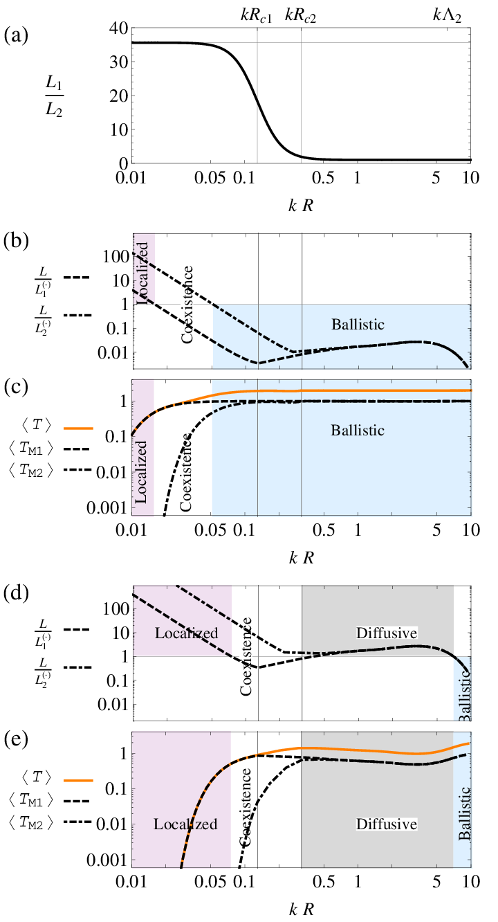
In order to discuss the dependence of the transmittances and their scaling parameters upon the dimensionless correlation length , Fig. 6 is presented. In the region , where intra-mode scattering prevails, the transmittances , , , the scaling parameters , , and the ratio of these parameters , are depicted. Otherwise, in the region , where inter-mode scattering prevails, the transmittances , , , the scaling parameters , , and the ratio , are depicted. In the first region the transmittances are computed from Eqs. (33) and (32), whereas in the second region, from Eqs. (51), (52). In both ranges, however, the scattering lengths are computed from Eqs. (23).
If decreases, the lengths and decreases as whereas the cycle length has a fixed value, thus, the smallest value of is restricted by the criterion (17a); here this criterion is fulfilled since and at the left boundary of the plots, . Because the plots illustrate the case of weak correlations (), the condition (17b) is satisfied automatically if (17a) is met.
The ratio of the lengths , which is equal to the ratio for , is in Fig. 6 (a). It exhibits the crossover from square-gradient scattering to gradient scattering. Therefore, with the increase of , the ratio decreases from the large value
| (63) |
to the unity,
| (64) |
The asymptotes (63) and (64) are obtained, respectively, through Eqs. (47) and (50). In contrast with the SRB waveguide, here the equality of mode-attenuation lengths, , emerges as a result of a strong intermode mixing, which is governed by the gradient-scattering mechanism. This non-trivial fact is in a strong contrast with a non-isotropic character of surface scattering in the channel space [13, 37].
In Fig. 6 (b)-(c) and (d)-(e) two cases are illustrated in which, depending upon the roughness correlation length , different transport regimes can arise. The first case corresponds to a moderately large waveguide that can present the localized, coexistence or ballistic transport regime; see frames (b) and (c). In comparison, the second case corresponds to a larger waveguide that can present the diffusive transport regime in addition to the aforementioned ones; see frames (d) and (e). Note that different transport regimes, defined in Eqs. (55), (57), (59) and (61), can be graphically identified with the use of frames (b) and (d) for the scaling parameters.
The total and mode transmittances are plotted in Figs. 6 (c) and (e). These plots demonstrate that, due to the hierarchy of mode-backscattering lengths, , the transmittance of the second mode is always smaller than the transmittance of the first one,
| (65) |
Therefore, within the localization (55) and coexistence (57) regions, the total transmittance (33) is mainly contributed by the first term, i.e. by the first-mode transmittance,
| (66) |
Within the localization regime, behaves as indicated in Eq. (56). Within the coexistence regime the total transmittance is described by Eq. (58). In the diffusive regime the mode transmittances are equal, and behave as indicated in Eq. (54). The total transmittance has twice their value, see Fig. 6 (e) and Eqs. (60). For the ballistic regime (61b), both conducting channels are open
| (67) |
Here the approximation given by Eq. (53) describes well the behavior of the mode transmittances. Correspondingly, the value of the total transmittance tends to the total number of the propagating modes, see Eq. (62).
Note that the coexistence transport regime arises if the length is such that , meanwhile the implied hierarchy emerges if the correlation length is smaller than the crossing point, . Therefore, in the ASRB waveguide the scattering governed by the square-gradient-scattering mechanism is a necessary condition for the coexistence transport regime to occur. In comparison, if the gradient-scattering mechanism prevails, the mode-attenuation lengths are almost equal, . Then, with a continuous increment of , the system passes directly from the ballistic to the diffusive regime.
IV.4 ASRB: Transmittance vs mode parameter
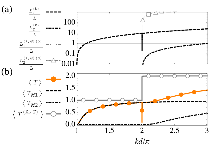
The mode-attenuation lengths and transmittances as functions of the mode parameter are presented in Fig. 7 within the range of first two modes. The value of the parameters are selected in order to illustrate, within the range , the coexistence transport regime of the ASRB waveguide, which is defined by Eq. (57).
Fig. 7 (a) shows the plots of and . Here is computed from Eqs. (23) and (23), whereas is given by the first term of the above equations, i.e.,
If increases, all the attenuation lengths also increase but exhibit characteristic dips at where a new normal mode opens. As we already noted, we can only indicate the position of these dips and do not describe their line shape in the narrow vicinity of integer values (see short discussion of these resonances in connection with Fig. 4). In contrast with the SRB waveguide, the curves depicting the first propagating mode of the ASRB waveguide show a dip at . This dip is caused by the inter-mode scattering from the first propagating mode into the second, and this scattering is governed by the gradient-scattering mechanism. Remarkably, far from the resonances at , the lengths and are larger than the mode-backscattering lengths, and . This is because of the main contribution of the square-gradient-scattering lengths, and . Therefore, the approximate behavior of is given by Eqs. (47a) and (47b)(not plotted in the Figure).
The total transmittance (33) and mode transmittances (32) are plotted in Fig. 7 (b). Note that the dips pertaining to the curves of and become evident in the curves for mode transmittances and . Certainly, the curve for the total transmittance incorporates all the dips of the mode transmittances. Remarkably, without the weight of the square-gradient scattering mechanism, both mode transmittances would have the same value and the total transmittance would have ballistic behavior. This fact can be graphically observed with the help of the curve related to the total transmittance given in Eq. (46), in which the square-gradient-scattering mechanism has been ignored.
V Conclusions
In this paper we report new results for transport properties of quasi-1D surface-disordered waveguides (or electronic conductors). Two models with symmetric and antisymmetric rough boundaries were studied in great detail. By examining these models, one passes from a system in which the attenuation of the propagating modes is associated with solely intra-mode scattering (the SRB waveguide), to a system in which both intra- and inter-mode scattering determine its attenuation (the ASRB waveguide). The comparison between the two models allows us to elucidate the role of all surface-scattering mechanisms.
As was shown in our previous analytical studies [17, 18, 19, 20, 21], one of mechanisms of scattering (the so-called square-gradient mechanism) is typically neglected in the literature since it emerges in the second order of perturbation theory. Specifically, the corresponding term in the expression for the inverse attenuation length is proportional to the squared variance of disorder, , and for this reason the square-gradient terms seem to be much smaller than the others describing conventional mechanisms of scattering (giving rise to the -dependence). However, apart from the dependence on the disorder strength, one has to take into account the correlation properties of scattering profiles. It was found that the square-gradient mechanism essentially depends on the correlations of different nature as compared with the -terms in the total expression for the inverse attenuation length.
In particular, it was argued that in some regions of parameters, the square-gradient terms can prevail the -terms and, therefore, have to be considered as well, in spite of their apparent smallness. These predictions have been carefully analyzed in this paper, within two models with symmetric and antisymmetric scattering profiles. Due to a principal difference between the two models, we analyze them separately.
For the SRB waveguide the transmission occurs along two modes independently, due to the underlying symmetry of the model. Therefore, the transport through each of two modes can be described in terms of standard theories of localization in one-dimensional models with random potentials. Thus, the total transmission is the sum of partial transmissions with the corresponding quantized transverse momentum. Our results demonstrate that in this case a typical situation occurs for which the transmission along two channels can be very different due to different values of corresponding backscattering lengths.
For the ASRB waveguide there exist a competition of two surface-scattering mechanism, which in contrast with the SRB waveguide, induce the interplay between intra-mod and inter-mode scattering. This is a challenging situation that persists with open questions. Nevertheless, the theoretical approach developed in Refs. 18, 20, 21 allows one to determine intervals of parameters in which only one of the above mechanisms plays the main role, i.e., it is possible to know when the channels can be considered as two independent one-dimensional conductors and when they exhibit a strong interaction. Moreover, that theoretical approach indicates a rather small region of transition between the above possibilities, where analytical results does not exist. The whole problem thus split off can be addressed by two complementary approaches. When the intra-mode scattering prevails the transport through the waveguide can be described by the theory proposed for the SRB waveguide but with the proper scaling parameters. When the inter-mode scattering prevails, it is necessary to apply the special approach developed here. Our results shows different transport regimes from localization to the ballistic, with the possibility, depending upon the waveguide parameters, of finding the coexistence and diffusive regimes. The coexistence regime can be present because of the hierarchy of mode-attenuation lengths associated with the square-gradient-scattering mechanism. Also, it is shown that the role of gradient mechanism of scattering is decisive, giving rise to a quite unexpected result. Specifically, it is demonstrated that in this case the partial transmissions along two channels are practically equal, and this effect is entirely due to the influence of the gradient terms in the expression for partial attenuation lengths. Due to the gradient-scattering mechanism that leads to the strong interaction between channels, the diffusive regime can take place.
Our results can help to understand specific properties of surface scattering in waveguides and electronic devices, in dependence on correlation properties of scattering profiles. In particular, one can understand the conditions under which the square-gradient mechanism of scattering has to be taken into account.
References
- [1] K. L. Chopra, Thin film phenomena (McGraw-Hill, New York, 1969).
- [2] A. A. Abrikosov and I. A. Ryzhkin, Advances in Physics, 27, 147 (1978).
- [3] R. Landauer, Physica Scripta, T42, 110 (1992).
- [4] S. Datta, Electronic Transport in Mesoscopic Systems (Cambridge University Press, Cambridge, 1995).
- [5] T. Dittrich, P. Hänggi, G.-L. Ingold, B. Kramer, G. Schön, and W. Zwerger, Quantum Transport and Dissipation (Wiley-VCH, Weinheim, 1998).
- [6] E. Akkermans and G. Montambaux, Mesoscopic Physics of Electrons and Photons (Cambridge University Press, Cambridge, 2007).
- [7] N. Trivedi and N. W. Ashcroft, Phys. Rev. B, 38, 12298 (1988).
- [8] Y. Takagaki and D. K. Ferry, J. Phys.: Condens. Matter, 4, 10421 (1992).
- [9] V. I. Kozub and A. A. Krokhin, J. Phys.: Condens. Matter, 5, 9135 (1993).
- [10] A. E. Meyerovich and S. Stepaniants, Phys. Rev. B, 51, 17116 (1995).
- [11] N. M. Makarov, A. V. Moroz, and V. A. Yampol’skii, Phys. Rev. B, 52, 6087 (1995).
- [12] A. García-Martín, J. A. Torres, J. J. Sáenz, and M. Nieto-Vesperinas, Phys. Rev. Lett. , 80, 4165 (1998).
- [13] J. A. Sánchez-Gil, V. Freilikher, I. V. Yurkevich, and A. A. Maradudin, Phys. Rev. Lett. , 80, 948 (1998).
- [14] J. A. Sánchez-Gil, V. Freilikher, A. A. Maradudin, and I. V. Yurkevich, Phys. Rev. B, 59, 5915 (1999).
- [15] E. Abrahams, P. W. Anderson, D. C. Licciardello, and T. V. Ramakrishnan, Phys. Rev. Lett., 42, 673 (1979).
- [16] F. M. Izrailev and N. M. Makarov, J. Phys. A: Math. Gen., 38, 10613 (2005).
- [17] F. M. Izrailev, N. M. Makarov, and M. Rendón, Phys. Rev. B, 72, 041403 (2005).
- [18] F. M. Izrailev, N. M. Makarov, and M. Rendón, Phys. Rev. B, 73, 155421 (2006).
- [19] M. Rendón, F. M. Izrailev, and N. M. Makarov, in Proceedings of The Sixth International Kharkov Symposium on Physics and Engineering of Microwaves Millimeter and Submillimeter Waves (MSMW’07), Vol. 1 (the Institute of Electrical and Electronics Engineers, 2007) pp. 131–136.
- [20] M. Rendón, F. M. Izrailev, and N. M. Makarov, Phys. Rev. B, 75, 205404 (2007b).
- [21] M. Rendón, F. M. Izrailev, and N. M. Makarov, in Proceedings of 12th International Conference on Mathematical Methods in Electromagnetic Theory (MMET*08) (the Institute of Electrical and Electronics Engineers, 2008) pp. 354–359.
- [22] F. G. Bass and I. M. Fuks, Wave Scattering from Statistically Rough Surfaces (Pergamon, New York, 1979).
- [23] J. A. DeSanto and G. S. Brown, “Analytical techniques for multiple scattering from rough surfaces,” (North Holland, Amsterdam, 1986) Chap. I.
- [24] J. A. Ogilvy, Theory of Wave Scattering from Random Rough Surfaces (Adam Hilger, Bristol, 1991).
- [25] V. D. Freilikher and S. A. Gredeskul, “Localization of waves in media with one-dimensional disorder,” (North Holland, Amsterdam, 1992) Chap. III.
- [26] I. Ohlídal, K. Navrátil, and M. Ohlídal, “Scattering of light from multilayer systems with rough boundaries,” (North Holland, Amsterdam, 1995) Chap. IV.
- [27] R. Kubo, J. Phys. Soc. Japan, 12, 570 (1957).
- [28] A. B. Migdal, Qualitative methods in quantum theory (Benjamin, London, 1977) p.98.
- [29] A. R. McGurn and A. A. Maradudin, Phys. Rev. B, 30, 3136 (1984).
- [30] N. M. Makarov and Y. V. Tarasov, Phys. Rev. B, 64, 235306(14) (2001).
- [31] V. L.Berezinski, Zh. Eksp. Teor. Fiz., 65, 1251 (1973), [Engl. Transl: Sov. Phys. JETP 38, 620 (1974)].
- [32] R. Bellman and G. M. Wing, An Introduction to Invariant Imbedding (Wiley, New York, 1975).
- [33] V. I. Klyatskin, The Invariant Imbedding Method in a Theory of Wave Propagation (Nauka, Moscow, 1986) in Russian, French Translation: Diffuseur, Editions de Physique.
- [34] N. M. Makarov and Y. V. Tarasov, J. Phys.: Condens. Matter, 10, 1523 (1998).
- [35] N. M. Makarov, “Lectures on spectral and transport properties of one-dimensional disordered conductors,” (1999), http://www.ifuap.buap.mx/virtual/page vir.html.
- [36] A. García-Martín, J. A. Torres, J. J. Sáenz, and M. Nieto-Vesperinas, Appl. Phys. Lett, 71, 1912 (1997).
- [37] A. García-Martín, J. J. Sáenz, and M. Nieto-Vesperinas, Phys. Rev. Lett. , 84, 3578 (2000).