Twisted Magnons

Preprint: YITP-SB-10-43

Abhijit Gadde Affiliation: abhijit@insti.physics.sunysb.edu Leonardo RastelliC.N. Yang Institute for Theoretical Physics,Stony Brook University,Stony Brook, NY 11794-3840, USA Affiliation: leonardo.rastelli@stonybrook.edu

Abstract:

We study spin chains for superconformal quiver gauge theories in the moduli space of ${\cal N}=2$ orbifolds. Independent of integrability, which is generally broken, we use the centrally extended $SU(2|2)$ symmetry of the magnons to fix their dispersion relations and two-body S-matrices, as functions of the exactly marginal couplings.

1 Introduction

The spin chain associated to the planar dilation operator of ${\cal N}=4$ super-Yang Mills [1, 2, 3] is strongly constrained by symmetry. While the structure of the Hamiltonian becomes unwieldy beyond one loop, and no closed form is yet in sight, the S-matrix of magnon excitations of the infinite chain is a relatively simple object [4, 5, 6]. Assuming integrability (for which there is by now strong evidence), the $n$ -body S-matrix factorizes in terms of two-body S-matrices. In turn, the full matrix structure of the two-body S-matrix is fixed by Beisert’s centrally extended $SU(2|2)\times SU(2|2)$ symmetry [5]. Finally, the overall phase is determined with the help of crossing symmetry and plausible physical assumptions [7, 8, 9, 10].

The centrally extended $SU(2|2)$ symmetry is a general feature of spin chains for ${\cal N}=2$ $4d$ superconformal theories¹¹ 1 See also [11] for applications of $SU(2|2)$ to a class theories with 16 supercharges., indeed $SU(2|2)$ is a subgroup of the ${\cal N}=2$ superconformal group $SU(2,2|2)$ preserved by the choice of the spin chain vacuum. In this paper we explore the consequences of this symmetry in a class of ${\cal N}=2$ SCFTs, the quiver theories related by exactly marginal deformations to ${\cal N}=2$ orbifolds of ${\cal N}=4$ super-Yang Mills.

Unlike the case of ${\cal N}=4$ SYM, only one copy of the $SU(2|2)$ supergroup is preserved, while the other is broken to its bosonic subgroup. We show how to fix the dispersion relations and two-body S-matrices of the magnons transforming under the surviving $SU(2|2)$ by a generalization of Beisert’s approach. Since the $SU(2|2)$ representations are now “twisted”, the generalization is not entirely trivial and leads to interesting functions of the exactly marginal couplings. At the orbifold point the magnons are gapless and the spin chain is integrable [12, 13] but as we perturb away from it, the magnons acquire a gap, and their two-body S-matrices do not satisfy the Yang-Baxter equation. So for general values of the couplings the theories are not integrable, and the complete magnon S-matrix cannot be deduced from the two-body S-matrix. Nevertheless the dispersion relations and two-body S-matrices are interesting pieces of information in their own right, and it is remarkable that one can obtain for them all-order expressions. At one-loop, we find agreement with the explicit perturbative calculations of [14, 15]. At strong ’t Hooft coupling, one should be able to compare our field-theoretic results with a giant-magnon [16] calculation in the dual string theory, which is a deformation of the orbifold background $AdS_{5}\times S^{5}/\Gamma$ [17, 18].

For ease of notation, in most of the paper we focus on the simplest case, the ${\cal N}=2$ superconformal quiver with $SU(N_{c})\times SU(N_{\check{c}})$ gauge group,²² 2 The two gauge groups are identical, $N_{c}\equiv N_{\check{c}}$ , but we find it useful to always denote with a “check” quantities associated to the second gauge group. which is in the moduli space of the $\mathbb{Z}_{2}$ orbifold of ${\cal N}=4$ SYM. In section 2 we determine the dispersion relation of the bifundamental magnons and in section 3 their two-body S-matrix.

Following Berenstein et al. [19], in section 4 we re-derive the dispersion relations of the twisted magnons from a large $N$ analysis of the quiver matrix model, obtained by quantizing the gauge theory on $S^{3}\times\mathbb{R}$ and keeping the zero modes on $S^{3}$ . It is not a priori obvious that this approach, which relies on an uncontrolled approximation, should give the same answer as the exact algebraic analysis, but it does. This viewpoint gives a simple geometric interpretation of dispersion relations, very suggestive of an emergent dual geometry.

The generalization to ${\cal N}=2$ $\mathbb{Z}_{k}$ orbifolds is straightforward, and we indicate it in section 5.

In the rest of this introduction we describe the symmetry structure of the $\mathbb{Z}_{2}$ -quiver spin chain, contrasting it with the ${\cal N}=4$ chain. This will serve as an overview of our logic and to orient the reader through our notations.

The superconformal symmetry of ${\cal N}=4$ SYM is $PSU(2,2|4)$ . It is broken to $PSU(2|2)\times PSU(2|2)\times\mathbb{R}$ , where $\mathbb{R}$ is a central generator corresponding to the spin chain Hamiltonian, by the choice of the BMN [20] vacuum ${\rm Tr}\,\Phi^{J}$ . The magnon excitations on this vacuum are in the fundamental representation of the unbroken symmetry, and they are gapless because they are the Goldstone modes associated to the broken generators. The $PSU(2,2|4)$ symmetry generators are shown in table 1. The boxed generators, in the diagonal blocks, are preserved by the choice of the vacuum while the off-diagonal ones are broken and correspond to the magnons. The broken generators are labelled in terms of the corresponding magnons: the upper-right block contains the magnon creation operators and the lower-left block the magnon annihilation operators.

	$SU(2_{\dot{\alpha}})$	$SU(2_{I})$	$SU(2_{\alpha})$	$SU(2_{\hat{I}})$
$SU(2_{\dot{\alpha}})$	$\mathcal{L}_{\>\dot{\beta}}^{\dot{\alpha}}$	$\mathcal{Q}_{\>J}^{\dot{\alpha}}$	$D_{\>\beta}^{\dagger\dot{\alpha}}$	$\lambda_{\>\hat{J}}^{\dagger\dot{\alpha}}$
$SU(2_{I})$	$\mathcal{S}_{\>\dot{\beta}}^{I}$	$\mathcal{R}_{\>J}^{I}$	$\lambda_{\>\beta}^{\dagger I}$	$\mathcal{X}_{\>\hat{J}}^{\dagger I}$
$SU(2_{\alpha})$	$D_{\>\dot{\beta}}^{\alpha}$	$\lambda_{\>J}^{\alpha}$	$\mathcal{L}_{\>\beta}^{\alpha}$	$\mathcal{Q}_{\>\hat{J}}^{\alpha}$
$SU(2_{\hat{I}})$	$\lambda_{\>\dot{\beta}}^{\hat{I}}$	$\mathcal{X}_{\>J}^{\hat{I}}$	$\mathcal{S}_{\>\beta}^{\hat{I}}$	$\mathcal{R}_{\>\hat{J}}^{\hat{I}}$

Table 1: The

PSU(2,2|4)

symmetry generators. The R-symmetry subgroup

SU(4)

is represented as branched into

SU(2_{I})\times SU(2_{\hat{I}})

. We have introduced the notation

SU(2_{\alpha})

for

SU(2)_{\alpha}

etc.

A priori, the two-body magnon S-matrix, decomposed according to the $SU(2_{\alpha}|2_{\hat{I}})\times SU(2_{\dot{\alpha}}|2_{I})$ quantum numbers, can take the schematic form

S_{SU(2_{\alpha}|2_{\hat{I}})\times SU(2_{\dot{\alpha}}|2_{I})}=S_{SU(2_{\alpha}|2_{\hat{I}})}\otimes S_{SU(2_{\dot{\alpha}}|2_{I})}+S_{SU(2_{\alpha}|2_{\hat{I}})}^{\prime}\otimes S_{SU(2_{\dot{\alpha}}|2_{I})}^{\prime}+\ldots

(1)

As it turns out, the $SU(2|2)$ S-matrix is unique up to an overall phase [5], so one has the useful factorization

S_{SU(2_{\alpha}|2_{\hat{I}})\times SU(2_{\dot{\alpha}}|2_{I})}=S_{SU(2_{\alpha}|2_{\hat{I}})}\otimes S_{SU(2_{\dot{\alpha}}|2_{I})}\,.

(2)

The $SU(2_{\alpha}|2_{\hat{I}})$ S-matrix describes the scattering of magnons in the highest weight state of $SU(2_{\dot{\alpha}}|2_{I})$ , and viceversa.

The $\mathbb{Z}_{2}$ projection of ${\cal N}=4$ SYM breaks $PSU(2_{\alpha},2_{\dot{\alpha}}|4_{I\hat{I}})$ to $SU(2_{\alpha},2_{\dot{\alpha}}|2_{I})\times SU(2_{\hat{I}})$ . At the orbifold point $g_{YM}=\check{g}_{YM}$ the breaking is only global (by boundary conditions on the periodic chain), but for general couplings the $PSU(2_{\alpha},2_{\dot{\alpha}}|4_{I\hat{I}})$ is truly lost. The symmetry preserved by the spin chain vacuum is $SU(2_{\dot{\alpha}}|2_{I})\times SU(2_{\alpha})\times SU(2_{\hat{I}})$ . Table 2 lists the symmetry generators of the theory, with the broken generators identified as Goldstone modes. The Goldstone excitations (gapless magnons) are in the fundamental representation of $SU(2_{\alpha})\times SU(2_{\dot{\alpha}}|2_{I})$ . The $\{\mathcal{X}_{\>\hat{J}}^{I}\,,\lambda_{\>\hat{J}}^{\dot{\alpha}}\}$ magnons, in the fundamental of $SU(2_{\hat{I}})\times SU(2_{\dot{\alpha}}|2_{I})$ , are omitted in table 2 because they do not correspond to broken generators – indeed they have a gap for $g_{YM}\neq\check{g}_{YM}$ . Their dynamics is the main focus of this paper.

Here we are using the “orbifold” notation, where the fields are labeled as in ${\cal N}=4$ SYM, and are $2N_{c}\times 2N_{c}$ matrices in color space (see equ.(2.2)). The state space of the spin chain consists of an twisted and and untwisted sector, distinguished by whether or not the twist operator $\tau$ (equ.(17)) is inserted on the chain. The two sectors mix for $g_{YM}\neq\check{g}_{YM}$ . In particular the symmetry generators and the central charges acquire twisted components, see (33, 34).

	$SU(2_{\dot{\alpha}})$	$SU(2_{I})$	$SU(2_{\alpha})$	$SU(2_{\hat{I}})$
$SU(2_{\dot{\alpha}})$	$\mathcal{L}_{\>\dot{\beta}}^{\dot{\alpha}}$	$\mathcal{Q}_{\>J}^{\dot{\alpha}}$	$D_{\>\beta}^{\dagger\dot{\alpha}}$
$SU(2_{I})$	$\mathcal{S}_{\>\dot{\beta}}^{I}$	$\mathcal{R}_{\>J}^{I}$	$\lambda_{\>\beta}^{\dagger I}$
$SU(2_{\alpha})$	$D_{\>\dot{\beta}}^{\alpha}$	$\lambda_{\>J}^{\alpha}$	$\mathcal{L}_{\>\beta}^{\alpha}$
$SU(2_{\hat{I}})$				$\mathcal{R}_{\>\hat{J}}^{\hat{I}}$

Table 2: The generators of

SU(2,2|2)\times SU(2_{\hat{I}})

, the symmetry of the

\mathbb{Z}_{2}

quiver. As before, the boxed generator are preserved by the choice of the spin-chain vacuum while the other correspond to Goldstone excitations.

The scattering of any two magnons (gapless or gapped) is given by a factorized two-body S-matrix,

S_{SU(2_{\alpha})\times SU(2_{\hat{I}})\times SU(2_{\dot{\alpha}}|2_{I})}={S}_{SU(2_{\alpha})\times SU(2_{\hat{I}})}\otimes S_{SU(2_{\dot{\alpha}}|2_{I})}\,.

(3)

The $S_{SU(2_{\dot{\alpha}}|2_{I})}$ S-matrix describes the scattering of magnons in the highest weight of $SU(2_{\alpha})\times SU(2_{\hat{I}})$ . It has both an untwisted and a twisted component, schematically

S_{SU(2_{\dot{\alpha}}|2_{I})}\,|{\cal X}_{1}{\cal X}_{2}\rangle={\cal S}^{\mathbb{I}}\,|{\cal X}_{1}{\cal X}_{2}\rangle+{\cal S}^{\tau}\,|{\cal X}_{1}{\cal X}_{2}\tau\rangle\,.

(4)

The centrally extended $SU(2|2)$ symmetry will fix both components uniquely, up to the usual phase ambiguity.

2 Magnon Dispersion Relations

2.1 Review: ${\cal N}=4$ magnons

The field content of ${\cal N}=4$ super Yang-Mills consists of the gauge field $A_{\mu}$ , four Weyl spinors $\lambda_{\alpha}^{A}$ and six real scalars $X^{i}$ , where $A=1,\ldots 4$ and $i=1,\ldots 6$ are indices labelling fundamental and antisymmetric self-dual representation of the $SU(4_{A})$ R-symmetry group respectively. Under $U(1)_{r}\times SU(2_{I})_{R}\times SU(2_{\hat{I}})_{L}\subset SU(4_{A})$ , the scalars branch into one complex scalar $\Phi$ , charged under $U(1)_{r}$ , and $SU(2_{I})_{R}\times SU(2_{\hat{I}})_{L}$ bifundamental scalars ${\cal X}^{I\hat{I}}$ , with zero $U(1)_{r}$ charge, satisfying the reality condition ${\cal X}^{I\hat{I}\dagger}=-\epsilon^{IJ}\epsilon^{\hat{I}\hat{J}}{\cal X}^{J\hat{J}}$ . The fermions decompose as $\lambda_{\alpha}^{I}$ and $\lambda_{\alpha}^{\hat{I}}$ . The ${\cal N}=2$ supersymmetry organizes $A_{\mu},\lambda_{\alpha}^{I},\Phi$ into a vector multiplet and ${\cal X}^{I\hat{I}},\lambda_{\alpha}^{\hat{I}}$ into a hypermultiplet.

For definiteness we focus on the “right-handed” magnons, in the fundamental of $SU(2_{\dot{\alpha}}|2_{I})$ and in the highest-weight state of of $SU(2_{\alpha}|2_{\hat{I}})$ ,

\mathcal{X}_{\>\hat{+}}^{I}\equiv\mathcal{X}^{I}\,,\quad\lambda_{\>\hat{+}}^{\dot{\alpha}}\equiv\lambda^{\dot{\alpha}}\,.

(5)

Beisert determined the magnon dispersion relation from symmetry arguments, as we now review. The non-zero commutation relations of the $SU(2|2)$ generators are:

$\displaystyle[\mathcal{R}_{\>J}^{I},\mathcal{J}^{K}]$	$\displaystyle=$	$\displaystyle\delta_{J}^{K}\mathcal{J}^{I}-\frac{1}{2}\delta_{J}^{I}\mathcal{J}^{K}$
$\displaystyle{}[\mathcal{L}_{\>\dot{\beta}}^{\dot{\alpha}},\mathcal{J}^{\dot{\gamma}}]$	$\displaystyle=$	$\displaystyle\delta_{\>\dot{\beta}}^{\dot{\gamma}}\mathcal{J}^{\dot{\alpha}}-\frac{1}{2}\delta_{\dot{\beta}}^{\dot{\alpha}}\mathcal{J}^{\dot{\gamma}}$
$\displaystyle\{\mathcal{Q}_{\>I}^{\dot{\alpha}},\mathcal{S}_{\>\dot{\beta}}^{J}\}$	$\displaystyle=$	$\displaystyle\delta_{I}^{J}\mathcal{L}_{\>\dot{\beta}}^{\dot{\alpha}}+\delta_{\dot{\beta}}^{\dot{\alpha}}\mathcal{R}_{\>I}^{J}+\delta_{I}^{J}\delta_{\dot{\beta}}^{\dot{\alpha}}\mathcal{C}$

where $\mathcal{J}$ represents any generator with the appropriate index. The central charge $\mathcal{C}$ is related to the scaling dimension as $\mathcal{C}=\frac{1}{2}(\Delta-|r|)$ . The impurities $({\cal X}^{\cal I}\,,\lambda^{\dot{\alpha}})$ transform in the fundamental representation of $SU(2|2)$ , and closure of the algebra fixes $\mathcal{C}=\frac{1}{2}$ , corresponding to the canonical dimensions $\Delta=1$ and $\Delta=\frac{3}{2}$ for ${\cal X}$ and $\lambda$ . Consider now a magnon of momentum $p$ ,

\Psi(p)=\sum_{l=-\infty}^{\infty}e^{ipl}|\mathcal{X}(l)\,\rangle.

(6)

For $p\neq 0$ , the state acquires a non-vanishing anomalous dimension, so $\mathcal{C}\neq\frac{1}{2}$ , but the representation remains short, as there are no other degrees of freedom with which it could combine to become long. This is in conflict with the $SU(2|2)$ algebra. The resolution is to allow for a further central extension by momentum-dependent central charges $\mathcal{P}$ and $\mathcal{K}$ ,

\{\mathcal{Q}_{\>I}^{\dot{\alpha}},\mathcal{Q}_{\>J}^{\dot{\beta}}\}=\epsilon^{\dot{\alpha}\dot{\beta}}\epsilon_{IJ}\mathcal{P},\quad\{\mathcal{S}_{\>\dot{\alpha}}^{I},\mathcal{S}_{\>\dot{\beta}}^{J}\}=\epsilon^{IJ}\epsilon_{\dot{\alpha}\dot{\beta}}\mathcal{K}\,.

(7)

The most general action of the generators in the excitation picture is :

$\displaystyle\mathcal{Q}_{\>I}^{\dot{\alpha}}\|\mathcal{X}^{J}\rangle$	$\displaystyle=$	$\displaystyle a\delta_{I}^{J}\|\lambda^{\dot{\alpha}}\rangle$	(8)
$\displaystyle\mathcal{Q}_{\>I}^{\dot{\alpha}}\|\lambda^{\dot{\beta}}\rangle$	$\displaystyle=$	$\displaystyle b\epsilon^{\dot{\alpha}\dot{\beta}}\epsilon_{IJ}\|\mathcal{X}^{J}\Phi^{+}\rangle$
$\displaystyle\mathcal{S}_{\>\dot{\alpha}}^{I}\|\mathcal{X}^{J}\rangle$	$\displaystyle=$	$\displaystyle c\epsilon^{IJ}\epsilon_{\dot{\alpha}\dot{\beta}}\|\lambda^{\dot{\beta}}\Phi^{-}\rangle$
$\displaystyle\mathcal{S}_{\>\dot{\alpha}}^{I}\|\lambda^{\dot{\beta}}\rangle$	$\displaystyle=$	$\displaystyle d\delta_{\dot{\alpha}}^{\dot{\beta}}\|\mathcal{X}^{I}\rangle\,,$

which implies

$\displaystyle\mathcal{P\|}\mathcal{X}\rangle$	$\displaystyle=$	$\displaystyle ab\|\mathcal{X}\Phi^{+}\rangle$	(9)
$\displaystyle\mathcal{K\|}\mathcal{X}\rangle$	$\displaystyle=$	$\displaystyle cd\|\mathcal{X}\Phi^{-}\rangle\,.$	(10)
$\displaystyle\mathcal{C}\|\mathcal{X}\rangle$	$\displaystyle=$	$\displaystyle\frac{1}{2}(ad+bc)\|\mathcal{X}\rangle\,.$	(11)

Closure of the algebra requires $ad-bc=1$ . We can then formally solve

\mathcal{C}=\frac{1}{2}\sqrt{1+4\mathcal{P}\mathcal{K}}\,.

(12)

For a quick heuristic derivation of the central charges, we can proceed as follows. The supersymmetry transformations of the fields appearing in the Lagrangian,

	$\displaystyle\mathcal{Q}_{\>I}^{\dot{\alpha}}\mathcal{X}^{K}$	$\displaystyle=$	$\displaystyle\delta_{I}^{K}\lambda^{\dot{\alpha}}$
	$\displaystyle\mathcal{Q}_{\>J}^{\dot{\beta}}\lambda^{\dot{\alpha}}$	$\displaystyle=$	$\displaystyle\epsilon^{\dot{\beta}\dot{\alpha}}\frac{\partial W}{\partial\mathcal{X}^{J}}=\frac{g}{\sqrt{2}}\epsilon^{\dot{\beta}\dot{\alpha}}\epsilon_{JL}[\mathcal{X}^{L},\Phi]$

where $W=\frac{g}{\sqrt{2}}\mbox{Tr }\mathcal{X}^{I\hat{I}}\Phi\mathcal{X}_{I\hat{I}}$ is the superpotential of ${\cal N}=4$ super Yang-Mills. The coupling $g$ is the square root of the ’t Hooft coupling, normalized as

g^{2}=\frac{g_{YM}^{2}N_{c}}{8\pi^{2}}\,.

(13)

These susy transformations lead to the anticommutators

	$\displaystyle\{\mathcal{Q}_{\>I}^{\dot{\alpha}},\mathcal{Q}_{\>J}^{\dot{\beta}}\}\mathcal{X}^{K}$	$\displaystyle=$	$\displaystyle\frac{g}{\sqrt{2}}\epsilon^{\dot{\alpha}\dot{\beta}}\epsilon_{IJ}[\Phi,\mathcal{X}^{K}]$
	$\displaystyle\{\mathcal{Q}_{\>I}^{\dot{\alpha}},\mathcal{Q}_{\>J}^{\dot{\beta}}\}\lambda^{\dot{\gamma}}$	$\displaystyle=$	$\displaystyle\frac{g}{\sqrt{2}}\epsilon^{\dot{\alpha}\dot{\beta}}\epsilon_{IJ}[\Phi,\lambda^{\dot{\gamma}}]$

Using the fact that momentum eigenstates satisfy

|\Phi^{\pm}\mathcal{X}\rangle=e^{\mp ip}|\mathcal{X}\Phi^{\pm}\rangle\,,

(14)

we can realize the susy transformation laws on the spin chain as

\{\mathcal{Q}_{\>I}^{\dot{\alpha}},\mathcal{Q}_{\>J}^{\dot{\beta}}\}|\mathcal{X}\rangle=\epsilon^{\dot{\alpha}\dot{\beta}}\epsilon_{IJ}\mathcal{P}|\mathcal{X}\rangle=\epsilon^{\dot{\alpha}\dot{\beta}}\epsilon_{IJ}\frac{g}{\sqrt{2}}(e^{-ip}-1)|\mathcal{X}\Phi^{+}\rangle\,,

(15)

implying $ab=\frac{g}{\sqrt{2}}(e^{-ip}-1)$ . Similarly using $\{\mathcal{S},\mathcal{S}\}$ , we can obtain $cd=\frac{g}{\sqrt{2}}(e^{ip}-1)$ . Finally, from (12),

\Delta-|r|=2\mathcal{C}=\sqrt{1+8g^{2}\sin^{2}\frac{p}{2}}\,.

(16)

This derivation³³ 3 The first field-theoretic argument for the square-root form (16) was given in [21]. is only heuristic because of the assumption that the susy transformations in the excitation picture can be simply read off from the classical Lagrangian. In [5], Beisert used a purely algebraic method to determine the central charges, as we review in appendix A. The algebraic method confirms the form (16), but with $g^{2}$ a priori replaced by a renormalized coupling ${\bf g}^{2}=g^{2}+O(g^{4})$ . There is strong evidence that in ${\cal N}=4$ SYM ${\bf g}^{2}=g^{2}$ . In the ABJM theory [22] one can run an identical argument, but the coupling is renormalized [23, 24, 25]. See [26, 27] for discussions of this issue.

2.2 The $\mathbb{Z}_{2}$ orbifold and its deformation

The $\mathbb{Z}_{2}$ orbifold theory is the well known quiver gauge theory living on the worldvolume of D3 branes probing $\mathbb{R}^{2}\times\mathbb{R}^{4}/\mathbb{Z}_{2}$ singularity. It is obtained from ${\cal N}=4$ super Yang-Mills by projecting onto the $\mathbb{Z}_{2}\subset SU(2)_{L}$ invariant states. The $\mathbb{Z}_{2}$ action identifies $\mathcal{X}^{I\hat{I}}\to-{\cal X}^{I\hat{I}}$ while acting trivially on $\Phi$ . The supersymmetry is broken to ${\cal N}=2$ as the supercharges with $SU(2)_{L}$ indices are projected out. The $SU(4)$ R symmetry group is broken to $SU(2)_{R}\times SO(3)_{L}\times U(1)_{r}$ . $SU(2)_{R}\times U(1)_{r}$ is the R symmetry group of the ${\cal N}=2$ theory while $SO(3)_{L}$ is a global symmetry. In color space, we start with $SU(2N_{c})$ gauge group and declare the nontrivial element of the orbifold to be

\tau=\left(\begin{array}[]{cc}\mathbb{I}_{N_{c}\times N_{c}}&0\\ 0&-\mathbb{I}_{N_{\check{c}}\times N_{\check{c}}}\end{array}\right).

(17)

It acts on the fields of ${\cal N}=4$ SYM as

A_{\mu}\to\tau A_{\mu}\tau,\qquad\Phi\to\tau\Phi\tau,\qquad\lambda^{I}\to\tau\lambda^{I}\tau,\qquad{\cal X}^{I\hat{I}}\to-\tau{\cal X}^{I\hat{I}}\tau,\qquad\lambda^{\hat{I}}\to-\tau\lambda^{\hat{I}}\tau.

(18)

The components that survive the projection are

	$\displaystyle A_{\mu}$	$\displaystyle=$	$\displaystyle\left(\begin{array}[]{cc}A_{\mu}&0\\ 0&\check{A}_{\mu}\end{array}\right),\quad\Phi=\left(\begin{array}[]{cc}\phi&0\\ 0&\check{\phi}\end{array}\right),\quad\lambda^{I}=\left(\begin{array}[]{cc}\lambda^{I}&0\\ 0&\check{\lambda}^{I}\end{array}\right),$
	$\displaystyle{\cal X}^{I\hat{I}}$	$\displaystyle=$	$\displaystyle\left(\begin{array}[]{cc}0&Q^{I\hat{I}}\\ \bar{Q}^{I\hat{I}}&0\end{array}\right),\quad\lambda^{\hat{I}}=\left(\begin{array}[]{cc}0&\psi^{\hat{I}}\\ \tilde{\psi}^{\hat{I}}&0\end{array}\right).$

The orbifold theory has an untwisted sector of states, which descend by projection from ${\cal N}=4$ , and a twisted sector of states, characterized by the presence of one insertion of the twist operator $\tau$ in the color trace. We refer to this presentation of the theory (in terms of $2N_{c}\times 2N_{c}$ matrices) as the “orbifold basis”.

Equivalently, we can present the theory as an ${\cal N}=2$ quiver gauge theory with product gauge group $SU(N_{c})\times SU(N_{\check{c}})$ and two bifundamental hypermultiplets: $(A_{\mu},\lambda^{I},\phi)$ and $(\check{A}_{\mu},\check{\lambda},\check{\phi})$ are the two vector multiplets while $(Q^{I\hat{I}},\psi^{\hat{I}})$ and $(\bar{Q}^{I\hat{I}},\tilde{\psi}^{\hat{I}})$ are the two hypermultiplets transforming respectively in the ${\bf N}_{c}\times\overline{{\bf N}}_{\check{c}}$ and $\overline{{\bf N}}_{c}\times{\bf N}_{\check{c}}$ representations.

The two gauge couplings $g$ and $\check{g}$ are exactly marginal. For $g\neq\check{g}$ the superpotential acquires a twisted term,

W=\frac{G}{\sqrt{2}}\mbox{Tr }[\frac{1}{2}(\sqrt{\kappa}+\frac{1}{\sqrt{\kappa}})+\tau\frac{1}{2}(\sqrt{\kappa}-\frac{1}{\sqrt{\kappa}})]\mathcal{X}^{I\hat{I}}\Phi\mathcal{X}_{I\hat{I}}

(31)

where

G\equiv\sqrt{g\check{g}}\,,\qquad\kappa\equiv\frac{\check{g}}{g}\,.

(32)

In the quiver language,

	$\displaystyle W$	$\displaystyle=$	$\displaystyle\frac{g}{\sqrt{2}}\mbox{Tr }\bar{Q}^{I\hat{I}}\phi Q_{I\hat{I}}+\frac{\check{g}}{\sqrt{2}}Q^{I\hat{I}}\check{\phi}\bar{Q}_{I\hat{I}}$
		$\displaystyle=$	$\displaystyle\frac{G}{\sqrt{2}}(\mbox{Tr }\frac{1}{\sqrt{\kappa}}\bar{Q}^{I\hat{I}}\phi Q_{I\hat{I}}+\sqrt{\kappa}Q^{I\hat{I}}\check{\phi}\bar{Q}_{I\hat{I}})\,.$

2.3 Twisted magnons

As we have explained in the introduction, the magnons of the $\mathbb{Z}_{2}$ theory fall into two classes: Goldstone magnons associated with the broken generators, carrying an $\alpha$ index, and magnons not associated with symmetries, carrying a $\hat{I}$ index. Both types are in the fundamental representation of $SU(2_{\dot{\alpha}}|2_{I})$ . The algebraic analysis for the Goldstone magnons is exactly as in ${\cal N}=4$ SYM, so they obey the same dispersion relation. On the other hand, the non-Goldstone magnons transform in a “twisted” representation of the $SU(2|2)$ superalgebra,

$\displaystyle\mathcal{Q}_{\>I}^{\dot{\alpha}}\|\mathcal{X}^{J}\rangle$	$\displaystyle=$	$\displaystyle a_{0}\delta_{I}^{J}\|\lambda^{\dot{\alpha}}\rangle+a_{1}\delta_{I}^{J}\|\tau\lambda^{\dot{\alpha}}\rangle$	(33)
$\displaystyle\mathcal{Q}_{\>I}^{\dot{\alpha}}\|\lambda^{\dot{\beta}}\rangle$	$\displaystyle=$	$\displaystyle b_{0}\epsilon^{\dot{\alpha}\dot{\beta}}\epsilon_{IJ}\|\mathcal{X}^{J}\Phi^{+}\rangle+b_{1}\epsilon^{\dot{\alpha}\dot{\beta}}\epsilon_{IJ}\|\tau\mathcal{X}^{J}\Phi^{+}\rangle$
$\displaystyle\mathcal{S}_{\>\dot{\alpha}}^{I}\|\mathcal{X}^{J}\rangle$	$\displaystyle=$	$\displaystyle c_{0}\epsilon^{IJ}\epsilon_{\dot{\alpha}\dot{\beta}}\|\lambda^{\dot{\beta}}\Phi^{-}\rangle+c_{1}\epsilon^{IJ}\epsilon_{\dot{\alpha}\dot{\beta}}\|\tau\lambda^{\dot{\beta}}\Phi^{-}\rangle$
$\displaystyle\mathcal{S}_{\>\dot{\alpha}}^{I}\|\lambda^{\dot{\beta}}\rangle$	$\displaystyle=$	$\displaystyle d_{0}\delta_{\dot{\alpha}}^{\dot{\beta}}\|\mathcal{X}^{I}\rangle+d_{1}\delta_{\dot{\alpha}}^{\dot{\beta}}\|\tau\mathcal{X}^{I}\rangle$

One then finds for the central charges:

$\displaystyle\mathcal{P}\|\mathcal{X}\rangle$	$\displaystyle=$	$\displaystyle(a_{0}b_{0}+a_{1}b_{1})\|\mathcal{X}\Phi^{+}\rangle+(a_{0}b_{1}+a_{1}b_{0})\|\tau\mathcal{X}\Phi^{+}\rangle$	(34)
$\displaystyle\mathcal{K}\|\mathcal{X}\rangle$	$\displaystyle=$	$\displaystyle(c_{0}d_{0}+c_{1}d_{1})\|\mathcal{X}\Phi^{-}\rangle+(c_{0}d_{1}+c_{1}d_{0})\|\tau\mathcal{X}\Phi^{-}\rangle$
$\displaystyle\mathcal{C}\|{\cal X}\rangle$	$\displaystyle=$	$\displaystyle[\frac{1}{2}(a_{0}d_{0}+b_{0}c_{0})+\frac{1}{2}(a_{1}d_{1}+b_{1}c_{1})]\|{\cal X}\rangle$
	$\displaystyle+$	$\displaystyle[\frac{1}{2}(a_{0}d_{1}+b_{0}c_{1})+\frac{1}{2}(a_{1}d_{0}+b_{1}c_{0})]\|\tau{\cal X}\rangle\,.$

Using the supersymmetry transformations following from the deformed superpotential (31), a little calculation gives

$\displaystyle a_{0}b_{0}+a_{1}b_{1}$	$\displaystyle=$	$\displaystyle\frac{G}{\sqrt{2}}\frac{1}{2}(\frac{1}{\sqrt{\kappa}}+\sqrt{\kappa})(e^{-ip}-1)$	(35)
$\displaystyle a_{0}b_{1}+a_{1}b_{0}$	$\displaystyle=$	$\displaystyle\frac{G}{\sqrt{2}}\frac{1}{2}(\frac{1}{\sqrt{\kappa}}-\sqrt{\kappa})(e^{-ip}+1)$
$\displaystyle c_{0}d_{0}+c_{1}d_{1}$	$\displaystyle=$	$\displaystyle\frac{G}{\sqrt{2}}\frac{1}{2}(\frac{1}{\sqrt{\kappa}}+\sqrt{\kappa})(e^{ip}-1)$
$\displaystyle c_{0}d_{1}+c_{1}d_{0}$	$\displaystyle=$	$\displaystyle\frac{G}{\sqrt{2}}\frac{1}{2}(\frac{1}{\sqrt{\kappa}}-\sqrt{\kappa})(e^{ip}+1)\,.$

We can then read off the central charges

	$\displaystyle C_{0}$	$\displaystyle\equiv$	$\displaystyle\frac{1}{2}(a_{0}d_{0}+b_{0}c_{0})+\frac{1}{2}(a_{1}d_{1}+b_{1}c_{1})=\frac{1}{2}\sqrt{1+8G^{2}\left(\sin^{2}\frac{p}{2}+\frac{1}{4}(\sqrt{\kappa}-\frac{1}{\sqrt{\kappa}})^{2}\right)}$
	$\displaystyle C_{1}$	$\displaystyle\equiv$	$\displaystyle\frac{1}{2}(a_{0}d_{1}+b_{0}c_{1})+\frac{1}{2}(a_{1}d_{0}+b_{1}c_{0})=0\,.$

It is illuminating to repeat the exercise in the quiver basis, as it will give us the dispersion relation of the perhaps more “physical” bifundamental excitations that interpolate between the ${\rm Tr}\,\phi^{J}$ and ${\rm Tr}\check{\phi}^{J}$ vacua. In the quiver basis, the $({\cal X},\,\lambda)$ doublet splits into two doublets, $(Q,\,\psi)$ and $(\bar{Q},\,\tilde{\psi})$ . Let us call these two fundamental $SU(2|2)$ representations $V$ and $\tilde{V}$ . The action of the algebra ${\cal A}:V\to V$ and ${\cal A}:\tilde{V}\to\tilde{V}$ is given in table 3.

$\begin{array}[]{ccccccc}\mathcal{Q}_{\>I}^{\dot{\alpha}}|Q^{J}\rangle&=&a\delta_{I}^{J}|\psi^{\dot{\alpha}}\rangle&&\mathcal{Q}_{\>I}^{\dot{\alpha}}|\bar{Q}^{J}\rangle&=&\tilde{a}\delta_{I}^{J}|\tilde{\psi}^{\dot{\alpha}}\rangle\\ \mathcal{Q}_{\>I}^{\dot{\alpha}}|\psi^{\dot{\beta}}\rangle&=&b\epsilon^{\dot{\alpha}\dot{\beta}}\epsilon_{IJ}|Q^{J}\check{\phi}^{+}\rangle&&\mathcal{Q}_{\>I}^{\dot{\alpha}}|\tilde{\psi}^{\dot{\beta}}\rangle&=&\tilde{b}\epsilon^{\dot{\alpha}\dot{\beta}}\epsilon_{IJ}|\bar{Q}^{J}\phi^{+}\rangle\\ \mathcal{S}_{\>\dot{\alpha}}^{I}|Q^{J}\rangle&=&c\epsilon^{IJ}\epsilon_{\dot{\alpha}\dot{\beta}}|\psi^{\dot{\beta}}\check{\phi}^{-}\rangle&&\mathcal{S}_{\>\dot{\alpha}}^{I}|\bar{Q}^{J}\rangle&=&\tilde{c}\epsilon^{IJ}\epsilon_{\dot{\alpha}\dot{\beta}}|\tilde{\psi}^{\dot{\beta}}\phi^{-}\rangle\\ \mathcal{S}_{\>\dot{\alpha}}^{I}|\psi^{\dot{\beta}}\rangle&=&d\delta_{\dot{\alpha}}^{\dot{\beta}}|Q^{I}\rangle&&\mathcal{S}_{\>\dot{\alpha}}^{I}|\tilde{\psi}^{\dot{\beta}}\rangle&=&\tilde{d}\delta_{\dot{\alpha}}^{\dot{\beta}}|\bar{Q}^{I}\rangle.\end{array}$

Table 3: Representation of the magnons in the quiver basis.

The $a,b,c,d$ coefficients in this basis are related to the coefficients in the orbifold basis as $a=a_{0}+a_{1}$ , $\tilde{a}=a_{0}-a_{1}$ and so on. One easily finds

	$\displaystyle ab$	$\displaystyle=$	$\displaystyle\frac{G}{\sqrt{2}}(\frac{e^{-ip}}{\sqrt{\kappa}}-\sqrt{\kappa})\equiv P\qquad\qquad\tilde{a}\tilde{b}=\frac{G}{\sqrt{2}}(e^{-ip}\sqrt{\kappa}-\frac{1}{\sqrt{\kappa}})\equiv\tilde{P}$		(36)
	$\displaystyle cd$	$\displaystyle=$	$\displaystyle\frac{G}{\sqrt{2}}(\frac{e^{+ip}}{\sqrt{\kappa}}-\sqrt{\kappa})\equiv K\qquad\qquad\tilde{c}\tilde{d}=\frac{G}{\sqrt{2}}(e^{+ip}\sqrt{\kappa}-\frac{1}{\sqrt{\kappa}})\equiv\tilde{K}\,.$

Finally the dispersion relations for $(Q,\psi)$ and $(\bar{Q}.\tilde{\psi})$ are

	$\displaystyle\Delta-\|r\|=2C$	$\displaystyle=$	$\displaystyle\sqrt{1+4PK}=\sqrt{1+8G^{2}\left(\sin^{2}\frac{p}{2}+\frac{1}{4}(\sqrt{\kappa}-\frac{1}{\sqrt{\kappa}})^{2}\right)}$		(37)
	$\displaystyle\tilde{\Delta}-\|r\|=2\tilde{C}$	$\displaystyle=$	$\displaystyle\sqrt{1+4\check{P}\check{K}}=\sqrt{1+8G^{2}\left(\sin^{2}\frac{p}{2}+\frac{1}{4}(\sqrt{\kappa}-\frac{1}{\sqrt{\kappa}})^{2}\right)}\,.$		(38)

Recall the definitions $G\equiv\sqrt{g\check{g}}$ , $\kappa\equiv\check{g}/g$ . As expected, the non-Goldstone magnons acquire a gap for $g\neq\check{g}$ . The derivation of the dispersion relation just presented suffers from the same criticism as the derivation in the ${\cal N}=4$ case: a priori we should allow for renormalization of the gauge couplings. A purely algebraic method for determining $\mathcal{P}$ and $\mathcal{K}$ , along the lines of [5], is described in the appendix A, and confirms this expectation. From symmetry alone, one can only conclude that both dispersion relations take the form

2C=2\check{C}=\sqrt{1+2({\bf g}-{{\bf\check{g}}})^{2}+8{\bf g\check{g}}\sin^{2}\frac{p}{2}}

(39)

where ${\bf g}(g,\check{g})=g+\dots$ and ${\bf\check{g}}(g,\check{g})=\check{g}+\dots$ are a priori renormalized couplings. (Of course such renormalization is known to not occur at the orbifold point $g=\check{g}$ .) This issue also affects the forthcoming expressions for the S-matrix: the couplings $g$ and $\check{g}$ could in principle be replaced by $\bf g$ and $\bf\check{g}$ . The expansion of (39) agrees at one-loop with the result of [14]. It will be interesting to test it at higher orders.

3 Two-body S-matrix

The scattering problem is formulated on the infinite spin chain. The scattering of two Goldstone magnons is uninteresting, since the matrix structure of their two-body S-matrix is exactly as in ${\cal N}=4$ SYM. We will focus on the scattering of two “non-Goldstone” magnons, both in the highest weight of $SU(2_{\hat{I}})$ . The scattering of a Goldstone and a non-Goldstone magnon is also non-trivial, and could be studied by the same methods.

In the quiver basis, because of the index structure of the impurities, one of the non-Goldstone magnons must be from the $Q$ multiplet and the other from the $\bar{Q}$ multiplet. Their ordering is fixed, we can have $Q$ type magnons always on left of $\bar{Q}$ type ones, or viceversa. The scattering is pure reflection. For the case of $Q$ type magnon on the left of $\bar{Q}$ type magnon, the schematic asymptotic form of the two body wavefunction is

\sum_{x_{1}\ll x_{2}}(e^{ip_{1}x_{1}+ip_{2}x_{2}}+S(p_{2},p_{1})e^{ip_{2}x_{1}+ip_{1}x_{2}})|\ldots\phi Q(x_{1})\check{\phi}\ldots\check{\phi}\bar{Q}(x_{2})\phi\ldots\rangle.

(40)

This is the definition of the two body S matrix $S(p_{1},p_{2})$ . We dropped the $SU(2|2)$ indices of the excitations for clarity. Similarly, for the other case where $Q$ is on the right side of $\bar{Q}$ , the aymptotic form of the wavefunction is

\sum_{x_{1}\ll x_{2}}(e^{ip_{1}x_{1}+ip_{2}x_{2}}+\check{S}(p_{2},p_{1})e^{ip_{2}x_{1}+ip_{1}x_{2}})|\ldots\check{\phi}\bar{Q}(x_{1})\phi\ldots\phi Q(x_{2})\check{\phi}\ldots\rangle

(41)

which defines $\check{S}$ . The two-body S matrices $S$ and $\check{S}$ are related by exchanging $g\leftrightarrow\check{g}$ ,

S(p_{1},p_{2};g,\check{g})=\check{S}(p_{1},p_{2};\check{g},g).

(42)

For this reason, without loss of generality, we restrict our analysis to finding $S(p_{1},p_{2})$ .

3.1 Rapidity variables

Following Beisert, a preliminary step is to solve for the coefficients $a,b,c,d$ and $\tilde{a},\tilde{b},\tilde{c},\tilde{d}$ appearing in the magnon representation (table 3) in terms of convenient rapidity variables.

For the representation coefficients of the $Q$ multiplet, we write

a=\gamma,\qquad b=-\frac{G}{\sqrt{2}}\frac{1}{\gamma x^{+}}(x^{+}\sqrt{\kappa}-\frac{x^{-}}{\sqrt{\kappa}}),\qquad c=\frac{G}{\sqrt{2}}\frac{i\gamma^{\prime}}{x^{-}},\qquad d=-\frac{i}{\gamma^{\prime}}(\frac{x^{+}}{\sqrt{\kappa}}-x^{-}\sqrt{\kappa})

(43)

The relative factor between $\gamma$ and $\gamma^{\prime}$ corresponds to relative rescalings of the fields $Q$ and $\psi$ and affects the S matrix as an overall phase. We choose $\gamma=\gamma^{\prime}$ .

For the $\bar{Q}$ coefficients, we write

\tilde{a}=\tilde{\gamma},\qquad\tilde{b}=-\frac{G}{\sqrt{2}}\frac{1}{\tilde{\gamma}\tilde{x}^{+}}(\frac{\tilde{x}^{+}}{\sqrt{\kappa}}-\tilde{x}^{-}\sqrt{\kappa}),\qquad\tilde{c}=\frac{G}{\sqrt{2}}\frac{i\tilde{\gamma}}{\tilde{x}^{-}},\qquad\tilde{d}=-\frac{i}{\tilde{\gamma}}(\tilde{x}^{+}\sqrt{\kappa}-\frac{\tilde{x}^{-}}{\sqrt{\kappa}}).

(44)

Both pairs of rapidity variables obey $\frac{x^{+}}{x^{-}}=\frac{\tilde{x}^{+}}{\tilde{x}^{-}}=e^{ip}$ . For hermitian representations we have to choose

|\gamma|=|i(x^{-}\sqrt{\kappa}-\frac{x^{+}}{\sqrt{\kappa}})|^{1/2},\qquad|\tilde{\gamma}|=|i(\frac{\tilde{x}^{-}}{\sqrt{\kappa}}-\tilde{x}^{+}\sqrt{\kappa})|^{1/2}.

(45)

The closure of the algebra requires $ad-bc=1$ and $\tilde{a}\tilde{d}-\tilde{b}\tilde{c}=1$ i.e.

	$\displaystyle\frac{x^{+}}{\sqrt{\kappa}}-x^{-}\sqrt{\kappa}+\frac{G^{2}}{2}(\frac{1}{x^{+}\sqrt{\kappa}}-\frac{\sqrt{\kappa}}{x^{-}})$	$\displaystyle=$	$\displaystyle i$
	$\displaystyle\tilde{x}^{+}\sqrt{\kappa}-\frac{\tilde{x}^{-}}{\sqrt{\kappa}}+\frac{G^{2}}{2}(\frac{\sqrt{\kappa}}{\tilde{x}^{+}}-\frac{1}{\tilde{x}^{-}\sqrt{\kappa}})$	$\displaystyle=$	$\displaystyle i.$

The central charges are then

	$\displaystyle\mathcal{C}$	$\displaystyle=$	$\displaystyle\frac{1}{2}+i\frac{G^{2}}{2}(\frac{1}{x^{+}\sqrt{\kappa}}-\frac{\sqrt{\kappa}}{x^{-}})=-i\frac{x^{+}}{\sqrt{\kappa}}+ix^{-}\sqrt{\kappa}-\frac{1}{2}$
	$\displaystyle\tilde{\mathcal{C}}$	$\displaystyle=$	$\displaystyle\frac{1}{2}+i\frac{G^{2}}{2}(\frac{\sqrt{\kappa}}{\tilde{x}^{+}}-\frac{1}{\tilde{x}^{-}\sqrt{\kappa}})=-i\tilde{x}^{+}\sqrt{\kappa}+i\frac{\tilde{x}^{-}}{\sqrt{\kappa}}-\frac{1}{2}.$

Although the expressions for the central charges (=anomalous dimensions) of $Q$ and $\bar{Q}$ look different in terms of rapidity variables $x$ and $\tilde{x}$ , they are in fact equal (by construction) as functions of the momenta.

3.2 The S-matrix

The S-matrix $S$ is an operator

S\,:\quad V\otimes\tilde{V}\to V\otimes\tilde{V}

(46)

and similarly

\check{S}\,:\quad\tilde{V}\otimes V\to\tilde{V}\otimes V\,.

(47)

The $SU(2|2)$ algebra acts on $V\otimes\tilde{V}$ as follows,

{\cal{\cal A}}(v\times\tilde{v})=({\cal A}v)\times\tilde{v}+(-1)^{F_{{\cal A}}F_{v}}v\times({\cal A}\tilde{v})\,,

(48)

where ${\cal A}$ is an element of the algebra, $v,\tilde{v}$ vectors in $V$ and $\tilde{V}$ , and $F$ the fermion number. To guarantee the $SU(2|2)$ symmetry of the S-matrix we simply need to impose the matrix equation $[{\cal A},S]=0$ . This is sufficient to determine $S$ up to an overall phase.

Following [5], we parametrize the S-matrix as

$\displaystyle S\|Q_{1}^{I}\bar{Q}_{2}^{J}\rangle$	$\displaystyle=$	$\displaystyle A\|Q_{2}^{\{I}\bar{Q}_{1}^{J\}}\rangle+B\|Q_{2}^{[I}\bar{Q}_{1}^{J]}\rangle+\frac{1}{2}C\epsilon^{IJ}\epsilon_{\dot{\alpha}\dot{\beta}}\|\psi_{2}^{\dot{\alpha}}\tilde{\psi}_{1}^{\dot{\beta}}\phi^{-}\rangle$
$\displaystyle S\|\psi_{1}^{\dot{\alpha}}\tilde{\psi}_{2}^{\dot{\beta}}\rangle$	$\displaystyle=$	$\displaystyle D\|\psi_{2}^{\{\dot{\alpha}}\tilde{\psi}_{1}^{\dot{\beta}\}}\rangle+E\|\psi_{2}^{[\dot{\alpha}}\tilde{\psi}_{1}^{\dot{\beta}]}\rangle+\frac{1}{2}F\epsilon^{\dot{\alpha}\dot{\beta}}\epsilon_{IJ}\|Q_{2}^{I}\bar{Q}_{1}^{J}\phi^{+}\rangle$
$\displaystyle S\|Q_{1}^{I}\tilde{\psi}_{2}^{\dot{\beta}}\rangle$	$\displaystyle=$	$\displaystyle G\|\psi_{2}^{\dot{\beta}}\bar{Q}_{1}^{I}\rangle+H\|Q_{2}^{I}\tilde{\psi}_{1}^{\dot{\beta}}\rangle$
$\displaystyle S\|\psi_{1}^{\dot{\alpha}}\bar{Q}_{2}^{J}\rangle$	$\displaystyle=$	$\displaystyle K\|\psi_{2}^{\dot{\alpha}}\bar{Q}_{1}^{J}\rangle+L\|Q_{2}^{J}\tilde{\psi}_{1}^{\dot{\alpha}}\rangle.$	(49)

The linear constraints obeyed by the S-matrix are listed in equ.(86). Below we give the solution for the components $A,\,B,\,C,\,G,\,H,\,K,\,L$ . The solution for $B,\,D$ and $E$ involve lengthier expressions – they can be readily obtained from equ.(86) with Mathematica’s help.

$\displaystyle A$	$\displaystyle=$	$\displaystyle\frac{\tilde{x}_{1}^{-}x_{2}^{-}}{x_{1}^{-}\tilde{x}_{2}^{-}}(\frac{\tilde{x}_{2}^{+}-x_{1}^{-}}{x_{2}^{-}-\tilde{x}_{1}^{+}})$	(50)
$\displaystyle B$	$\displaystyle=$	$\displaystyle\tilde{x}_{1}^{-}x_{2}^{-}[\tilde{x}_{1}^{+}x_{2}^{+}\kappa(2x_{2}^{-}x_{1}^{+}\tilde{x}_{2}^{+}-\tilde{x}_{1}^{+}x_{2}^{+}(x_{1}^{-}+\tilde{x}_{2}^{+}))$
		$\displaystyle+\tilde{x}_{1}^{-}(2\tilde{x}_{1}^{+}x_{2}^{+}(x_{1}^{-}x_{2}^{+}+\tilde{x}_{2}^{+}(x_{2}^{+}-x_{1}^{-}))$
		$\displaystyle+x_{2}^{-}(-2x_{1}^{+}\tilde{x}_{2}^{+}x_{2}^{+}+\kappa\tilde{x}_{1}^{+}(2x_{1}^{+}\tilde{x}_{2}^{+}-x_{2}^{+}(x_{1}^{-}+\tilde{x}_{2}^{+}))))]/$
		$\displaystyle\kappa\tilde{x}_{1}^{+}x_{2}^{+}x_{1}^{-}\tilde{x}_{2}^{-}(x_{2}^{-}-\tilde{x}_{1}^{+})(\tilde{x}_{1}^{-}x_{2}^{-}-\tilde{x}_{1}^{+}x_{2}^{+})$
$\displaystyle C$	$\displaystyle=$	$\displaystyle 2\sqrt{2}\tilde{\gamma}_{1}\gamma_{2}\tilde{x}_{1}^{-}x_{2}^{-}(\tilde{x}_{1}^{+}x_{2}^{+}(x_{1}^{-}+\tilde{x}_{2}^{+})-x_{1}^{+}\tilde{x}_{2}^{+}(x_{2}^{-}+\tilde{x}_{1}^{+}))/$
		$\displaystyle\kappa Gx_{1}^{-}\tilde{x}_{2}^{-}(x_{2}^{-}-\tilde{x}_{1}^{+})(\tilde{x}_{1}^{-}x_{2}^{-}-\tilde{x}_{1}^{+}x_{2}^{+})$
$\displaystyle G$	$\displaystyle=$	$\displaystyle\frac{\gamma_{2}}{\tilde{\gamma}_{2}}\frac{\tilde{x}_{1}^{-}x_{2}^{-}\tilde{x}_{2}^{+}}{x_{1}^{-}\tilde{x}_{2}^{-}x_{2}^{+}}(\frac{x_{2}^{+}-x_{1}^{+}}{x_{2}^{-}-\tilde{x}_{1}^{+}})$
$\displaystyle H$	$\displaystyle=$	$\displaystyle\frac{\tilde{\gamma}_{1}\tilde{x}_{1}^{-}x_{2}^{-}\tilde{x}_{2}^{+}}{\tilde{\gamma}_{2}x_{1}^{-}\tilde{x}_{2}^{-}x_{2}^{+}\tilde{x}_{1}^{+}}(\frac{\tilde{x}_{1}^{+}x_{2}^{+}-x_{2}^{-}x_{1}^{+}}{x_{2}^{-}-\tilde{x}_{1}^{+}})$
$\displaystyle K$	$\displaystyle=$	$\displaystyle\frac{\gamma_{2}\tilde{x}_{1}^{-}x_{2}^{-}}{\gamma_{1}x_{1}^{-}\tilde{x}_{2}^{-}x_{2}^{+}}(\frac{x_{1}^{+}\tilde{x}_{2}^{+}-x_{1}^{-}x_{2}^{+}}{x_{2}^{-}-\tilde{x}_{1}^{+}})$
$\displaystyle L$	$\displaystyle=$	$\displaystyle\frac{\tilde{\gamma}_{1}}{\gamma_{1}}\frac{\tilde{x}_{1}^{-}x_{2}^{-}}{x_{1}^{-}\tilde{x}_{2}^{-}\tilde{x}_{1}^{+}x_{2}^{+}}(\frac{x_{2}^{-}x_{1}^{+}\tilde{x}_{2}^{+}-x_{1}^{-}\tilde{x}_{1}^{+}x_{2}^{+}}{x_{2}^{-}-\tilde{x}_{1}^{+}})$

The Yang-Baxter equation fails to hold for $g\neq\check{g}$ , as already observed in the one-loop result of [14].

One-loop limit

At one-loop, going back to the momentum representation, the S-matrix simplifies to

$\displaystyle A$	$\displaystyle=$	$\displaystyle E\,=-\frac{1+e^{ip_{1}+ip_{2}}-2\kappa e^{ip_{2}}}{1+e^{ip_{1}+ip_{2}}-2\kappa e^{ip_{1}}}$	(51)
$\displaystyle B$	$\displaystyle=$	$\displaystyle D\,=-1$
$\displaystyle C$	$\displaystyle=$	$\displaystyle F\,=0$
$\displaystyle G$	$\displaystyle=$	$\displaystyle L\,=-\frac{\kappa(e^{ip_{1}}-e^{ip_{2}})}{1+e^{ip_{1}+ip_{2}}-2\kappa e^{ip_{1}}}$
$\displaystyle H$	$\displaystyle=$	$\displaystyle K\,=-\frac{1+e^{ip_{1}+ip_{2}}-\kappa(e^{ip_{1}}+e^{ip_{2}})}{1+e^{ip_{1}+ip_{2}}-2\kappa e^{ip_{1}}}$

The S-matrix $\check{S}$ for $\bar{Q}Q$ scattering is given by sending $\kappa\to\frac{1}{\kappa}$ in the above expressions.

The bosonic and fermionic impurities do not mix at one-loop. The $Q$ $\bar{Q}$ S-matrix agrees with the explicit perturbative calculation of [14]. The fermion S-matrix has also been successfully checked against one-loop perturbation theory [15].

All-loops at $\kappa=0$

For $\kappa=0$ , the all-loop $S$ matrix at $\kappa=0$ in the $Q\bar{Q}$ channel is rather trivial,

$\displaystyle A$	$\displaystyle=$	$\displaystyle E\,=-1$	(52)
$\displaystyle B$	$\displaystyle=$	$\displaystyle D\,=-1$
$\displaystyle C$	$\displaystyle=$	$\displaystyle F\,=0$
$\displaystyle G$	$\displaystyle=$	$\displaystyle L\,=0$
$\displaystyle H$	$\displaystyle=$	$\displaystyle K\,=-1\,.$

This is intuitively clear: the $Q$ and $\bar{Q}$ impurities are separated by adjoint fields in the “checked” vector multiplet, which decouples in the limit $\kappa\to 0$ .

On the other hand, in the $\bar{Q}Q$ scattering sector the scattering retains a a non-trivial dependence on the coupling (now the impurities are separated by the interacting fields of the “unchecked” vector multiplet),

$\check{A}=-e^{i(p_{2}-p_{1})}$	$\check{D}=-1$
$\check{B}=-e^{i(p_{2}-p_{1})}(\cos(p_{1}-p_{2})-i\frac{\sin(p_{1}-p_{2})}{\sqrt{1+2g^{2}}})\qquad$	$\check{E}=-(\cos(p_{1}-p_{2})+i\frac{\sin(p_{1}-p_{2})}{\sqrt{1+2g^{2}}})$
$\check{C}=-ie^{ip_{2}}\sqrt{2}g\frac{\sin(p_{1}-p_{2})}{\sqrt{1+2g^{2}}}$	$\check{F}=-ie^{-ip_{1}}\sqrt{2}g\frac{\sin(p_{1}-p_{2})}{\sqrt{1+2g^{2}}}$
$\check{G}=\frac{1}{2}(1-e^{i(p_{2}-p_{1})})$	$\check{L}=\frac{1}{2}(1-e^{i(p_{2}-p_{1})})$
$\check{H}=-\frac{1}{2}(1+e^{i(p_{2}-p_{1})})$	$\check{K}=-\frac{1}{2}(1+e^{i(p_{2}-p_{1})})$ .

The limit $\kappa\to 0$ is interesting because the $\mathbb{Z}_{2}$ quiver theory reduces to ${\cal N}=2$ superconformal QCD (plus the decoupled “checked” vector multiplet). We refer to [28, 14] for detailed discussions. For $\kappa=0$ the global symmetry $SU(2_{\hat{I}})$ combines with the second gauge group $SU(N_{\check{c}})$ and there is a symmetry enhancement to the flavor group $U(N_{f}=2N_{c})$ .

An important question is whether the flavor-singlet sector of the SCQQD spin-chain is integrable. We may now look forward to shed new light on this question using the above all-loop results. Unfortunately, flavor singlets are in particular $SU(2_{\hat{I}})$ singlets, and the methods of this paper only allow us to consider scattering of $SU(2_{\hat{I}})$ triplets. So our results have no direct bearing on the question of integrability of the ${\cal N}=2$ SQCD spin-chain. With this caveat, we may nevertheless go ahead and check whether the Yang-Baxter equation holds at $\kappa=0$ for $SU(2_{\hat{I}})$ triplets. It doesn’t.⁴⁴ 4 In [14], it was found that in the scalar sector, at one-loop, the YB equation holds as $\kappa\to 0$ both for $SU(2_{\hat{I}})$ triplets and $SU(2_{\hat{I}})$ singlets. Only the result for singlets is relevant to the integrability question.

4 Emergent Magnons

In [19], following [29], Berenstein et al. reproduced the all-loop magnon dispersion relation in ${\cal N}=4$ SYM using a simple matrix quantum mechanics. The matrix quantum mechanics is obtained by truncating to the lowest modes of $SU(N_{c})$ ${\cal N}=4$ SYM on $S^{3}$ . The ground state is obtained by minimizing the potential energy, which leads to a model of commuting hermitian matrices. The matrix eigenvalues are localized on a five-sphere of radius⁵⁵ 5 Our normalization for the fields are related to the normalization in [19] as $\phi_{here}=\phi_{there}/\sqrt{N_{c}}$ . $\frac{1}{\sqrt{2}}$ , which is naturally identified with the $S^{5}$ in the dual background. This gives a simple picture for emergent geometry. Each point in the emergent geometry corresponds to an eigenvalue and is labelled by an $SU(N_{c})$ index. In [30, 31] the same exercise for orbifolds of ${\cal N}=4$ SYM shows that the ground state of the matrix model is localized on the orbifolded $S^{5}$ .

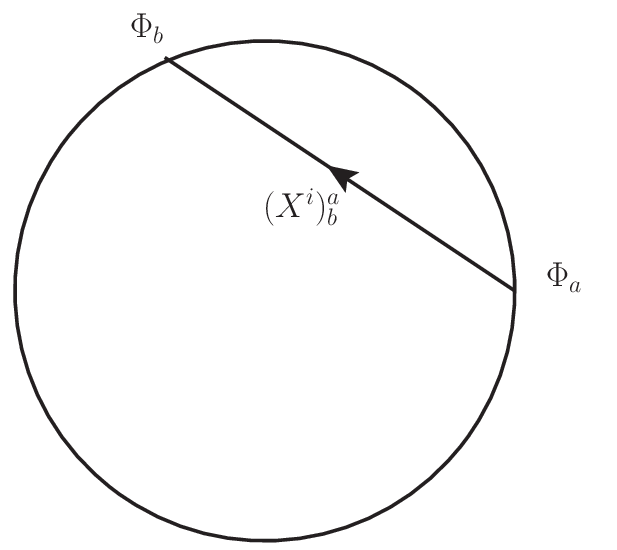
The excitations of the vacuum obtained by turning on off-diagonal modes of the matrix model are interpreted as string bits. They are bilocal in the emergent geometry because they are labelled by two $SU(N_{c})$ indices and are visualized as string bits stretching between two points (see figure 1). An off-diagonal excitation of momentum $p$ is peaked at the configuration where the corresponding string bit subtends an angle $p$ at the center. The expectation value of their energy precisely reproduces the exact magnon dispersion relation [19].

Refer to caption — Figure 1: The left figure shows the string bit corresponding to the off-diagonal excitation $(X^{i})^{a}_{b}$ . The right figure shows the configuration where the wavefunction of a magnon with momentum $p$ is peaked.

A very similar picture for the magnons was obtained in [16] on the dual string side. Moreover, the $x_{1}$ and $x_{2}$ components of the vector $\vec{M}$ associated with the magnon were identified with the central charges of the $SU(2|2)$ algebra [16]

M_{1}=\frac{1}{2}(K+P)\,,\quad M_{2}=\frac{1}{2i}(K-P)\,.

(53)

4.1 Emergent magnons for the $\mathbb{Z}_{2}$ quiver

Following [19], we truncate the $\mathbb{Z}_{2}$ quiver theory to its lowest bosonic modes on $S^{3}$ , which gives us the matrix quantum mechanis

$\displaystyle S$	$\displaystyle=$	$\displaystyle N_{c}\int dt\,\mbox{Tr}\>\frac{1}{2}\left((D_{t}\phi)^{2}+(D_{t}\check{\phi})^{2}+(D_{t}Q^{I\hat{I}})^{2}-\phi^{2}-\check{\phi}^{2}-(Q^{I\hat{I}})^{2}\right)$	(54)
	$\displaystyle-$	$\displaystyle g^{2}\left([\phi,\bar{\phi}]^{2}+\sqrt{2}Q^{I\hat{I}}\bar{Q}_{I\hat{I}}(\phi\bar{\phi}+\bar{\phi}\phi)+Q^{I\hat{I}}\bar{Q}_{J\hat{I}}Q^{J\hat{J}}\bar{Q}_{I\hat{J}}-\frac{1}{2}Q^{I\hat{I}}\bar{Q}_{I\hat{I}}Q^{J\hat{J}}\bar{Q}_{J\hat{J}}\right)$
	$\displaystyle-$	$\displaystyle{\check{g}}^{2}\left([\check{\phi},\bar{\check{\phi}}]^{2}+\sqrt{2}\bar{Q}_{I\hat{I}}Q^{I\hat{I}}(\check{\phi}\bar{\check{\phi}}+\bar{\check{\phi}}\check{\phi})+\bar{Q}_{J\hat{I}}Q^{I\hat{I}}\bar{Q}_{I\hat{J}}Q^{J\hat{J}}-\frac{1}{2}\bar{Q}_{I\hat{I}}Q^{I\hat{I}}\bar{Q}_{J\hat{J}}Q^{J\hat{J}}\right)$
	$\displaystyle+$	$\displaystyle\sqrt{g\check{g}}\left(4Q^{I\hat{I}}\check{\phi}\bar{Q}_{I\hat{I}}\bar{\phi}+h.c.\right)+\frac{1}{N_{c}}(\mbox{double}-\mbox{ trace}).$

The mass terms arise due to the conformal couplings of the scalars to curvature of $S^{3}$ . The eigenvalue distribution of the ground state is same as that of the $\mathbb{Z}_{2}$ orbifold of ${\cal N}=4$ SYM. We now excite the off-diagonal mode $(Q^{I\hat{I}})_{\check{b}}^{a}$ . The linearized theory describing this excitation is the harmonic oscillator,

	$\displaystyle H$	$\displaystyle=$	$\displaystyle\frac{1}{2}(\Pi_{I\hat{I}})_{\check{b}}^{a}(\Pi^{I\hat{I}})_{a}^{\check{b}}+\frac{1}{2}\omega_{a\check{b}}(Q^{I\hat{I}})_{\check{b}}^{a}(\bar{Q}_{I\hat{I}})_{a}^{\check{b}}$
	$\displaystyle\omega_{a\check{b}}$	$\displaystyle=$	$\displaystyle 1+4\|g\phi_{a}-\check{g}\check{\phi}_{\check{b}}\|^{2}.$

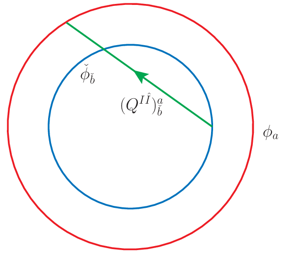
Note the difference in the frequency compared to the ${\cal N}=4$ case, where $\omega_{ab}=1+4g^{2}|\phi_{a}-\phi_{b}|^{2}$ . This motivates the effective picture of figure 2.

The circle spanned by the eigenvalues of $\Phi$ has split into two circles, one spanned by the eigenvalues of $\phi$ and the other by eigenvalues of $\check{\phi}$ . The radii of the two circles are taken to be $\frac{1}{\sqrt{\kappa}}\frac{G}{\sqrt{2}}$ and $\sqrt{\kappa}\frac{G}{\sqrt{2}}$ respectively, by normalizing the tension of the string bit to unity. The string bit corresponding to a bifundamental excitation stretches from one circle to the other. A magnon of momentum $p$ again localizes on the configuration where the string bit subtends an angle $p$ at the center. Using (53) we learn

{P}=x_{1}-ix_{2}=\frac{G}{\sqrt{2}}(e^{-ip}\frac{1}{\sqrt{\kappa}}-\sqrt{\kappa})={K}^{*}\,,

(55)

so the energy of the magnon is

\Delta-|r|=\sqrt{1+8G^{2}\left(\sin^{2}\frac{p}{2}+\frac{1}{4}(\sqrt{\kappa}-\frac{1}{\sqrt{\kappa}})^{2}\right)}.

(56)

The central charges agree precisely with the from obtained earlier from the algebraic method.⁶⁶ 6 Of course, as before, there is no guarantee that the couplings do not get renormalized. This caveat is all the more obvious in this approach, since integrating out massive modes would generically lead to such a renormalization.

It is clear that the adjoint excitations $\lambda$ and $D$ ( $\check{\lambda}$ and $\check{D}$ ) are string bits that stretch between two points of $\phi$ circle ( $\check{\phi}$ circle). Their dispersion relation coincides with the ${\cal N}=4$ SYM dispersion relation, as clear from the picture. A generic state of the spin chain is shown in figure 3.

At strong ’t Hooft coupling, Hofman and Maldacena [16] obtained the dual description of an ${\cal N}=4$ magnon as a semiclassical strings rotating on the $S^{2}\subset S^{5}$ . In LLM coordinates this “giant magnon” has precisely the shape of figure 1. The energy of the string was matched with the strong coupling limit of the exact magnon dispersion relation. (See also [32] for a sigma-model derivation of the $SU(2|2)$ central charges.) The ${\mathbb{Z}}_{2}$ quiver theory is dual to the $AdS_{5}\times S^{5}/{\mathbb{Z}}_{2}$ background. The ratio of the gauge couplings is related the period of the NSNS B-field through the collapsed two-cycle. It must be possible to reproduce the effective picture of figure 2 and the associated dispersion relation by studying the giant magnon solution in this background. This problem is under investigation [33].

4.2 Bound states

In addition to the elementary magnons with real momenta, the spectrum of the theory also contains bound states at some special complex values of the momenta. A two-magnon bound state occurs at the pole of the two-body S-matrix,

S(p_{1},p_{2})=\infty\qquad\mbox{with }\quad p_{1}=\frac{P}{2}-iq,\quad p_{2}=\frac{P}{2}+iq,\quad q>0\,.

(57)

Since $S(p_{2},p_{1})=1/S(p_{1},p_{2})\to 0$ , the asymptotic wavefunction becomes

e^{iP\frac{x_{1}+x_{2}}{2}-q|x_{2}-x_{1}|}.

(58)

A bound state has smaller energy than any state in the two particle continuum with the same total mometum $P$ . The exact dispersion relation of the bound states in ${\cal N}=4$ SYM was found in [34] and their S-matrix in [35]. The two-body S-matrix in the present case allows us to determine the bound state dispersion relation. Finding their S-matrix, however, would requires the four-body magnon S-matrix, which we cannot determine in the absence of integrability.

Let us first analyze the bound state of $Q^{+}$ (on the left of the chain) and $\bar{Q}^{+}$ (on the right). Their scattering matrix given in equ.(50),

A(p_{1},p_{2})=S_{12}^{0}\frac{\tilde{x}_{2}^{-}x_{1}^{-}}{x_{2}^{-}\tilde{x}_{1}^{-}}(\frac{\tilde{x}_{1}^{+}-x_{2}^{-}}{x_{1}^{-}-\tilde{x}_{2}^{+}})\,,

(59)

where $S_{12}^{0}$ is the overall dressing factor which is not determined by symmetries. Clearly there is a pole is at $x_{1}^{-}=\tilde{x}_{2}^{+}$ . We assume that this pole is not cancelled by a zero of the dressing factor. Following [36], we define the bound state rapidity variables as

X^{+}\equiv x_{1}^{+},\qquad X^{-}\equiv\tilde{x}_{2}^{-}\,.

(60)

Remarkably, at the pole they obey the relations

	$\displaystyle\frac{X^{+}}{X^{-}}$	$\displaystyle=$	$\displaystyle e^{iP}$
	$\displaystyle X^{+}-X^{-}+\frac{G^{2}}{2}(\frac{1}{X^{+}}-\frac{1}{X^{-}})$	$\displaystyle=$	$\displaystyle 2i\sqrt{\kappa}.$

The bound state dispersion relation can also be expressed completely in terms of $X^{\pm}$ ,

	$\displaystyle C_{Q\bar{Q}}$	$\displaystyle=$	$\displaystyle C_{1}+\tilde{C}_{2}=1+i\frac{G^{2}}{2\sqrt{\kappa}}(\frac{1}{X^{+}}-\frac{1}{X^{-}})$		(61)
		$\displaystyle=$	$\displaystyle\frac{1}{2}\sqrt{4+8g^{2}\sin^{2}\frac{p}{2}}.$		(61)

This dispersion is exactly the same as the one of the two-magnon bound states in ${\cal N}=4$ SYM. Thus the $Q\bar{Q}$ bound state can be elegantly represented as a string bit of “weight two” stretching between two points of the outer circle. The analogous exercise for the $\bar{Q}Q$ bound state gives the dispersion relation

C_{\bar{Q}Q}=\frac{1}{2}\sqrt{4+8\check{g}^{2}\sin^{2}\frac{p}{2}}\,.

(62)

This bound state is represented as a weight-two string bit stretching between two points of the inner circle.

As we vary the momentum $P$ of the bound state the pole $iq$ moves on the positive imaginary axis. For certain values of $P$ where $q$ approaches zero, the bound state is only marginally stable. This phenomenon does not occur in ${\cal N}=4$ SYM, the bound states of ${\cal N}=4$ are stable for all values of $P$ but this is not the case for the $\mathbb{Z}_{2}$ quiver theory. The marginal stability condition $q=0$ gives respectively for the $Q\bar{Q}$ and $\bar{Q}Q$ bound states

\kappa=\cos\frac{P}{2}\qquad\mbox{and}\qquad\frac{1}{\kappa}=\cos\frac{P}{2}

(63)

In the latter case, there is no solution which means that $\bar{Q}Q$ bound state is stable for all values of the momenta. On the other hand, the $Q\bar{Q}$ bound state on the other hand can decay at $P=2\arccos\kappa$ . These conclusions exactly match with results obtained at one loop in [14].

Geometrically, there is simple way of understanding the boud state decay, see figure 4. As the bound state string bit stretching in the outer circle (which means it is a $Q\bar{Q}$ bound state) touches the inner circle, its energy becomes manifestly equal to the sum of the energies of the constituents. Vanishing of the binding energy allows the $Q\bar{Q}$ state to decay. Simple trigonometry reveals the threshold momentum $P=2\arccos\kappa$ at this point. From this picture it is also immediate to see that the $\bar{Q}Q$ bound state is stable for all values of the momenta.

As we move around in the parameter space of the quiver gauge theory, at certain codimension one “walls”, the bound states of the elementary magnons decay. It would be interesting to understand bound state decay as a wall-crossing phenomenon in the dual sigma model.

5 Generalization to $\mathbb{Z}_{k}$ orbifolds

The analysis presented for the $\mathbb{Z}_{2}$ quiver can be extended to a general ADE ${\cal N}=2$ orbifold of ${\cal N}=4$ SYM. In this section we indicate the generalization for the (marginally deformed) $\mathbb{Z}_{k}$ orbifolds. The quiver gauge theory describing such an orbifold is shown in figure 5.

The superpotential at a generic point in the parameter space is

W=\frac{1}{\sqrt{2}}\sum_{i}g_{(i)}\left(\mbox{Tr}Q_{(i-1,i)}^{I}\phi_{(i)}\bar{Q}_{I(i,i-1)}+\mbox{Tr}\bar{Q}_{I(i+1,i)}\phi_{(i)}Q_{(i,i+1)}^{I}\right).

(64)

We impose the periodicity condition $i+k\sim i$ on the indices.

To compute the $SU(2|2)$ central charges for the representation of the $Q_{(i,i+1)}^{I}$ magnon we evaluate the anticommutator of two supersymmetries,

\{Q_{I}^{\dot{\alpha}},Q_{J}^{\dot{\beta}}\}Q_{(i,i+1)}^{K}=\epsilon^{\dot{\alpha}\dot{\beta}}\epsilon_{IJ}(\frac{g_{(i)}}{\sqrt{2}}\phi_{(i)}Q_{(i,i+1)}^{K}-\frac{g_{(i+1)}}{\sqrt{2}}Q_{(i,i+1)}^{K}\phi_{(i+1)})

(65)

which, on the spin chain, leads to

	$\displaystyle\{Q_{I}^{\dot{\alpha}},Q_{J}^{\dot{\beta}}\}\|Q_{(i,i+1)}^{K}\rangle$	$\displaystyle=$	$\displaystyle\epsilon^{\dot{\alpha}\dot{\beta}}\epsilon_{IJ}\frac{1}{\sqrt{2}}(g_{(i)}e^{-ip}-g_{(i+1)})\|Q_{(i,i+1)}^{K}\phi^{+}\rangle$
	$\displaystyle\Rightarrow\mathcal{P}$	$\displaystyle=$	$\displaystyle\frac{1}{\sqrt{2}}(g_{(i)}e^{-ip}-g_{(i+1)})=\mathcal{K}^{*}.$

Interchanging $g_{(i)}\leftrightarrow g_{(i+1)}$ gives us the central charges of the $\bar{Q}_{(i+1,i)}$ representation. In both cases we get the dispersion relation

\Delta-|r|=2\mathcal{C}=\sqrt{1+8G_{(i,i+1)}^{2}\left(\sin^{2}\frac{p}{2}+\frac{1}{4}(\sqrt{\kappa_{(i,i+1)}}-\frac{1}{\sqrt{\kappa_{(i,i+1)}}})^{2}\right)}\,.

(66)

Here we have defined

G_{(i,i+1)}=\sqrt{g_{(i)}g_{(i+1)}}\qquad\mbox{and}\qquad\kappa_{(i,i+1)}=\frac{g_{(i+1)}}{g_{(i)}}.

(67)

The dispersion relation of the adjoint magnons $\lambda_{(i)}$ and $D_{(i)}$ works the same way as ${\cal N}=4$ and is equal to

\Delta-|r|=2\mathcal{C}=\sqrt{1+8g_{(i)}^{2}\sin^{2}\frac{p}{2}}.

(68)

The picture presented in section 4 also generalizes to $\mathbb{Z}_{k}$ orbifolds, see figure 6. It consists of $k$ concentric circles which are labelled by $i$ , corresponding to the gauge group $SU(N_{c})_{i}$ . The radius of $i$ -th circle is $\frac{g_{(i)}}{\sqrt{2}}$ . The magnons in the adjoint of the $i$ -th node are represented by string bits that stretch between the $i$ -th circle, while the $SU(N)_{i}\times SU(N)_{i+1}$ bifundamental magnons correspond to string bits stretching from $i$ -th to $i+1$ -th circle. The dispersion relations of both adjoint and bifundamental magnons is summarized by the simple formula

\Delta-|r|=\sqrt{1+4\ell^{2}}

(69)

where $\ell$ is the length of the corresponding string bit. The two-body S-matrix is also fixed by the centrally extended $SU(2|2)$ symmetry, and can be obtained by straightforward extension of our analysis of the $\mathbb{Z}_{2}$ case.

Acknowledgements

It is a pleasure to thank David Berenstein, Nikolay Bobev, Pedro Liendo, Elli Pomoni, Pedro Vieira and Wenbin Yan for useful discussions. This work was supported in part by DOE grant DEFG-0292-ER40697 and by NSF grant PHY-0653351-001. Any opinions, findings, and conclusions or recommendations expressed in this material are those of the authors and do not necessarily reflect the views of the National Science Foundation.

Appendix A Algebraic constraints on the central charges

A.1 ${\cal N}=4$ super Yang-Mills

Let us review the logic used in [5] to constrain the central elements $\mathcal{P}$ and $\mathcal{K}$ . The action of $\mathcal{P}$ on a state with $K$ $\mathcal{X}$ -excitations with momenta $p_{1},\ldots p_{K}$ is

\mathcal{P|}\mathcal{X}_{1}\mathcal{X}_{2}\ldots\mathcal{X}_{K}\rangle=\sum_{k=1}^{K}a_{k}b_{k}\prod_{l=k+1}^{K}e^{-ip_{l}}|\mathcal{X}_{1}\mathcal{X}_{2}\ldots\mathcal{X}_{K}\Phi^{+}\rangle

(70)

On a physical state like the one above, the central charge must vanish. Since in the ${\cal N}=4$ case all the $\mathcal{X}$ -excitations belong to the same (fundamental) representation of $SU(2|2)$ , the central charge only depends upon the momentum and not on the type of excitation, and the only possibility is for the sum in (70) to telescope to zero on physical states,

a_{i}b_{i}=\alpha(e^{-ip_{i}}-1)\equiv P

(71)

with $\alpha$ being an undetermined constant. Here we use the fact that the total momentum of a physical state is zero. A similar exercise for $\mathcal{K}$ gives

c_{i}d_{i}=\beta(e^{ip_{i}}-1)\equiv K\,.

(72)

On a single-particle state,

\mathcal{P|}{\cal X}\rangle=\alpha(e^{ip}-1)|{\cal X}\Phi^{+}\rangle,\qquad\mathcal{K|}{\cal X}\rangle=\beta(e^{-ip}-1)|{\cal X}\Phi^{-}\rangle\,.

(73)

The hermiticity condition translates into $\alpha=\beta^{*}$ . Finally

C=\frac{1}{2}\sqrt{1+4PK}=\frac{1}{2}\sqrt{1+16\alpha\beta\sin^{2}\frac{p}{2}}\,.

(74)

Comparing with the one loop dispersion relation one finds $\alpha\beta=\frac{g^{2}}{2}+O(g^{4})\equiv\frac{{\bf g}^{2}}{2}$ .

A.2 $\mathbb{Z}_{2}$ quiver

A physical state is constructed by having alternating $Q$ and $\bar{Q}$ type impurities on a periodic spin chain. The central charge should vanish on such a state. To determine the central charges $\mathcal{P}$ and $\mathcal{K}$ as functions of magnon mometum, we follow same steps as before. The action of $\mathcal{P}$ and $\mathcal{K}$ is

	$\displaystyle\mathcal{P}\|Q_{1}{\bar{Q}}_{2}\ldots Q_{K-1}{\bar{Q}}_{K}\rangle$
	$\displaystyle=\,(a_{1}b_{1}(e^{-ip_{2}}\ldots e^{-ip_{K}})+\tilde{a}_{2}\tilde{b}_{2}(e^{-ip_{3}}\ldots e^{-ip_{K}})+\ldots+\tilde{a}_{K}\tilde{b}_{K})\|Q_{1}{\bar{Q}}_{2}\ldots Q_{K-1}{\bar{Q}}_{K}\phi^{+}\rangle$
	$\displaystyle\mathcal{K}\|Q_{1}{\bar{Q}}_{2}\ldots Q_{K-1}{\bar{Q}}_{K}\rangle$
	$\displaystyle=\,(c_{1}d_{1}(e^{ip_{2}}\ldots e^{ip_{K}})+\tilde{c}_{2}\tilde{d}_{2}(e^{ip_{3}}\ldots e^{ip_{K}})+\ldots+\tilde{c}_{K}\tilde{d}_{K})\|Q_{1}{\bar{Q}}_{2}\ldots Q_{K-1}{\bar{Q}}_{K}\phi^{-}\rangle.$

As before, let us define $P_{i}\equiv a_{i}b_{i},K_{i}\equiv c_{i}d_{i}$ and ${\tilde{P}}_{i}\equiv{\tilde{a}}_{i}{\tilde{b}}_{i},\tilde{K}_{i}\equiv\tilde{c}_{i}\tilde{d}_{i}$ . Now we impose

1.

Physical state condition:
$\mathcal{P}$ and $\mathcal{K}$ should vanish when the total momentum of the state is zero.
2.

BPS condition:
A BPS state of the interpolating theory is obtained from a BPS state of the orbifold by the substitution (in the one-loop approximation) $\check{\phi}\to\kappa\check{\phi}$ , $\kappa\equiv{\check{g}}/g$ (see the last paragraph of appendix B in [28]). At higher orders we may have a renormalized substitution $\check{\phi}\to\kappa^{\prime}\check{\phi}$ , $k^{\prime}\equiv{\bf\check{g}}/{\bf g}$ with ${\bf g}(g,\check{g})$ and ${\bf\check{g}}(g,\check{g})$ renormalized couplings. This means $Q(\bar{Q})$ moving with momentum $i\ln\kappa^{\prime}\,\,(-i\ln\kappa^{\prime})$ is chiral and we expect that $P_{i}K_{i}\,\,(\tilde{P}_{i}\tilde{K}_{i})$ should vanish on that state.
3.

Hermiticity:
$K=P^{*}$ and ${\tilde{K}}={\tilde{P}}^{*}$ .

From these condition it follows that

	$\displaystyle P$	$\displaystyle=$	$\displaystyle\alpha(e^{-ip}\frac{1}{\sqrt{\kappa^{\prime}}}-\sqrt{\kappa^{\prime}}),\qquad\qquad K=\alpha^{*}(e^{ip}\frac{1}{\sqrt{\kappa^{\prime}}}-\sqrt{\kappa^{\prime}}),$
	$\displaystyle\tilde{P}$	$\displaystyle=$	$\displaystyle{\alpha}(e^{-ip}\sqrt{\kappa^{\prime}}-\frac{1}{\sqrt{\kappa^{\prime}}}),\qquad\qquad\tilde{K}={\alpha}^{*}(e^{ip}\sqrt{\kappa^{\prime}}-\frac{1}{\sqrt{\kappa^{\prime}}}).$

( $\{P,K\}\leftrightarrow\{\tilde{P},\tilde{K}\}$ is of course also a solution since the conditions above make no intrinsic distinction between the $Q$ and $\bar{Q}$ impurities.) We then have

	$\displaystyle C=\frac{1}{2}\sqrt{1+4PK}$	$\displaystyle=$	$\displaystyle\frac{1}{2}\sqrt{1+16\|\alpha\|^{2}\Big(\sin^{2}\frac{p}{2}+\frac{1}{4}(\sqrt{\kappa^{\prime}}-\frac{1}{\sqrt{\kappa^{\prime}}})\Big)^{2}}\,$		(75)
	$\displaystyle\tilde{C}=\frac{1}{2}\sqrt{1+4\tilde{P}\tilde{K}}$	$\displaystyle=$	$\displaystyle\frac{1}{2}\sqrt{1+16\|\alpha\|^{2}\Big(\sin^{2}\frac{p}{2}+\frac{1}{4}(\sqrt{\kappa^{\prime}}-\frac{1}{\sqrt{\kappa^{\prime}}})\Big)^{2}}.$		(76)

Comparing with the one-loop dispersion relation [14] one finds $|\alpha|^{2}\equiv\frac{{\bf g\,\check{g}}}{2}=\frac{g\check{g}}{2}+\ldots$ . All in all,

C=\tilde{C}=\sqrt{1+2({\bf g}-{{\bf\check{g}}})^{2}+8{\bf g\check{g}}\sin^{2}\frac{p}{2}}\,.

(77)

Appendix B Solving for the S-matrix

$SU(2|1)$ subsector: Determining $A,\,K,\,G,\>H,\>L$

We first consider the $SU(2_{\dot{\alpha}}|1_{I})$ subsector, which is closed under scattering. Consider the scattering of two bosonic magnons $Q^{+}$ and $\bar{Q}^{+}$ . Requiring invariance under the supercharge ${\cal Q}_{+}^{\dot{\alpha}}$ we find

$\displaystyle\mathcal{Q}_{\,+}^{\dot{\alpha}}S_{12}\|Q_{1}^{+}\bar{Q}_{2}^{+}\rangle$	$\displaystyle=$	$\displaystyle\mathcal{Q}_{+}^{\dot{\alpha}}A_{12}\|Q_{2}^{+}\bar{Q}_{1}^{+}\rangle$
	$\displaystyle=$	$\displaystyle A_{12}a_{2}\|\psi_{2}^{\dot{\alpha}}\bar{Q}_{1}^{+}\rangle+A_{12}\tilde{a}_{1}\|Q_{2}^{+}\tilde{\psi}_{1}^{\dot{\alpha}}\rangle$
$\displaystyle S_{12}\mathcal{Q}_{\>+}^{\dot{\alpha}}\|Q_{1}^{+}\bar{Q}_{2}^{+}\rangle$	$\displaystyle=$	$\displaystyle S_{12}(a_{1}\|\psi_{1}^{\dot{\alpha}}\bar{Q}_{2}^{+}\rangle+\tilde{a}_{2}\|Q_{1}^{+}\tilde{\psi}_{2}^{\dot{\alpha}}\rangle)$
	$\displaystyle=$	$\displaystyle(a_{1}K_{12}+\tilde{a}_{2}G_{12})\|\psi_{2}^{\dot{\alpha}}\bar{Q}_{1}^{+}\rangle+(a_{1}L_{12}+\tilde{a}_{2}H_{12})\|Q_{2}^{+}\tilde{\psi}_{1}^{\dot{\alpha}}\rangle)$
$\displaystyle{}[\mathcal{Q}_{+}^{\dot{\alpha}},S]=0$	$\displaystyle\Rightarrow$
$\displaystyle A_{12}$	$\displaystyle=$	$\displaystyle\frac{a_{1}}{a_{2}}K_{12}+\frac{\tilde{a}_{2}}{a_{2}}G_{12}$
$\displaystyle A_{12}$	$\displaystyle=$	$\displaystyle\frac{a_{1}}{\tilde{a}_{1}}L_{12}+\frac{\tilde{a}_{2}}{\tilde{a}_{1}}H_{12}.$

More constraints are obtained by imposing invariance under conformal supersymmetries $\mathcal{S}$ . In this subsector it is sufficient to focus on $\mathcal{S}_{\dot{\alpha}}^{-}$ ,

$\displaystyle\mathcal{S}_{\>\dot{\alpha}}^{-}S_{12}\|Q_{1}^{+}\bar{Q}_{2}^{+}\rangle$	$\displaystyle=$	$\displaystyle A_{12}(-c_{2}\epsilon_{\dot{\alpha}\dot{\beta}}\|\psi_{2}^{\dot{\beta}}\check{\phi}^{-}\bar{Q}_{1}^{+}\rangle-\tilde{c}_{1}\epsilon_{\dot{\alpha}\dot{\beta}}\|Q_{2}^{+}\tilde{\psi}_{1}^{\dot{\beta}}\phi^{-}\rangle)$
	$\displaystyle=$	$\displaystyle A_{12}(-c_{2}\epsilon_{\dot{\alpha}\dot{\beta}}\frac{x_{2}^{-}}{x_{2}^{+}}\|\phi^{-}\psi_{2}^{\dot{\beta}}\bar{Q}_{1}^{+}\rangle-\tilde{c}_{1}\epsilon_{\dot{\alpha}\dot{\beta}}\frac{x_{2}^{-}\tilde{x}_{1}^{-}}{x_{2}^{+}\tilde{x}_{1}^{+}}\|\phi^{-}Q_{2}^{+}\tilde{\psi}_{1}^{\dot{\beta}}\rangle)$
$\displaystyle S_{12}\mathcal{S}_{\>\dot{\alpha}}^{+}\|Q_{1}^{+}\bar{Q}_{2}^{+}\rangle$	$\displaystyle=$	$\displaystyle S_{12}(-c_{1}\epsilon_{\dot{\alpha}\dot{\beta}}\frac{x_{1}^{-}}{x_{1}^{+}}\|\phi^{-}\psi_{1}^{\dot{\beta}}\bar{Q}_{2}^{+}\rangle-\tilde{c}_{2}\epsilon_{\dot{\alpha}\dot{\beta}}\frac{\tilde{x}_{2}^{-}x_{1}^{-}}{\tilde{x}_{2}^{+}x_{1}^{+}}\|\phi^{-}Q_{1}^{+}\tilde{\psi}_{2}^{\dot{\beta}}\rangle)$
	$\displaystyle=$	$\displaystyle-\epsilon_{\dot{\alpha}\dot{\beta}}(c_{1}\frac{x_{1}^{-}}{x_{1}^{+}}K_{12}+\tilde{c}_{2}\frac{\tilde{x}_{2}^{-}x_{1}^{-}}{\tilde{x}_{2}^{+}x_{1}^{+}}G_{12})\|\phi^{-}\psi_{2}^{\dot{\beta}}\bar{Q}_{1}^{+}\rangle$
	$\displaystyle-$	$\displaystyle\epsilon_{\dot{\alpha}\dot{\beta}}(c_{1}\frac{x_{1}^{-}}{x_{1}^{+}}L_{12}+\tilde{c}_{2}\frac{\tilde{x}_{2}^{-}x_{1}^{-}}{\tilde{x}_{2}^{+}x_{1}^{+}}H_{12})\|\phi^{-}Q_{1}^{+}\tilde{\psi}_{2}^{\dot{\beta}}\rangle\,.$

This gives another pair of constraints on the coefficients,

	$\displaystyle A_{12}$	$\displaystyle=$	$\displaystyle\frac{c_{1}}{c_{2}}\frac{x_{2}^{+}}{x_{2}^{-}}\frac{x_{1}^{-}}{x_{1}^{+}}K_{12}+\frac{\tilde{c}_{2}}{c_{2}}\frac{x_{2}^{+}}{x_{2}^{-}}\frac{\tilde{x}_{2}^{-}x_{1}^{-}}{\tilde{x}_{2}^{+}x_{1}^{+}}G_{12}$		(78)
	$\displaystyle A_{12}$	$\displaystyle=$	$\displaystyle\frac{c_{1}}{\tilde{c}_{1}}\frac{x_{2}^{+}}{x_{2}^{-}}\frac{\tilde{x}_{1}^{+}}{\tilde{x}_{1}^{-}}\frac{x_{1}^{-}}{x_{1}^{+}}L_{12}+\frac{\tilde{c}_{2}}{\tilde{c}_{1}}\frac{x_{2}^{+}}{x_{2}^{-}}\frac{\tilde{x}_{1}^{+}}{\tilde{x}_{1}^{-}}\frac{\tilde{x}_{2}^{-}x_{1}^{-}}{\tilde{x}_{2}^{+}x_{1}^{+}}H_{12}$		(79)

Bosonic singlet: Determining $B,\,C$

To evaluate the $B$ and $C$ matrix elements, we have to study the scattering of two bosons of opposite spins. Requiring $[\mathcal{Q}_{+}^{+},S]=0$ is sufficient to determine them. From

$\displaystyle{\cal\mathcal{Q}}_{+}^{+}S_{12}\|Q_{1}^{+}\bar{Q}_{2}^{-}\rangle$	$\displaystyle=$	$\displaystyle{\cal\mathcal{Q}}_{+}^{+}[(\frac{1}{2}A_{12}+\frac{1}{2}B_{12})\|Q_{2}^{+}\bar{Q}_{1}^{-}\rangle+(\frac{1}{2}A_{12}-\frac{1}{2}B_{12})\|Q_{2}^{-}\bar{Q}_{1}^{+}\rangle$
	$\displaystyle+$	$\displaystyle\frac{1}{2}C_{12}(\|\psi_{2}^{+}\tilde{\psi}_{1}^{-}\phi^{-}\rangle-\|\psi_{2}^{-}\tilde{\psi}_{1}^{+}\phi^{-}\rangle)]$
	$\displaystyle=$	$\displaystyle a_{2}(\frac{1}{2}A_{12}+\frac{1}{2}B_{12})\|\psi_{2}^{+}\bar{Q}_{1}^{-}\rangle+\tilde{a}_{1}(\frac{1}{2}A_{12}-\frac{1}{2}B_{12})\|Q_{2}^{-}\tilde{\psi}_{1}^{+}\rangle$
	$\displaystyle-$	$\displaystyle\tilde{b}_{1}\frac{1}{2}C_{12}\|\psi_{2}^{+}\bar{Q}_{1}^{-}\phi^{+}\phi^{-}\rangle-b_{2}\frac{1}{2}C_{12}\|Q_{2}^{-}\check{\phi}^{+}\tilde{\psi}_{1}^{+}\phi^{-}\rangle$
	$\displaystyle=$	$\displaystyle a_{2}(\frac{1}{2}A_{12}+\frac{1}{2}B_{12})\|\psi_{2}^{+}\bar{Q}_{1}^{-}\rangle+\tilde{a}_{1}(\frac{1}{2}A_{12}-\frac{1}{2}B_{12})\|Q_{2}^{-}\tilde{\psi}_{1}^{+}\rangle$
	$\displaystyle-$	$\displaystyle\tilde{b}_{1}\frac{1}{2}C_{12}\|\psi_{2}^{+}\bar{Q}_{1}^{-}\rangle-b_{2}\frac{1}{2}C_{12}\frac{\tilde{x}_{1}^{-}}{\tilde{x}_{1}^{+}}\|Q_{2}^{-}\tilde{\psi}_{1}^{+}\rangle$
$\displaystyle S_{12}{\cal\mathcal{Q}}_{+}^{+}\|Q_{1}^{+}\bar{Q}_{2}^{-}\rangle$	$\displaystyle=$	$\displaystyle S_{12}a_{1}\|\psi_{1}^{+}\bar{Q}_{2}^{-}\rangle$
	$\displaystyle=$	$\displaystyle a_{1}[K_{12}\|\psi_{2}^{+}\bar{Q}_{1}^{-}\rangle+L_{12}\|Q_{2}^{-}\tilde{\psi}_{1}^{+}\rangle]$

we find

	$\displaystyle a_{2}\frac{A_{12}+B_{12}}{2}-\tilde{b}_{1}\frac{C_{12}}{2}$	$\displaystyle=$	$\displaystyle a_{1}K_{12}$		(80)
	$\displaystyle\tilde{a}_{1}\frac{A_{12}-B_{12}}{2}-b_{2}\frac{\tilde{x}_{1}^{-}}{\tilde{x}_{1}^{+}}\frac{C_{12}}{2}$	$\displaystyle=$	$\displaystyle a_{1}L_{12}\,.$		(81)

We now turn to the scattering of fermions.

$SU(1|2)$ Subsector: Determining $D$

As before, we first focus on the $SU(1_{\dot{\alpha}}|2_{I})$ sector and consider the scattering of two fermions in the triplet of $SU(2)_{\dot{\alpha}}$ . This sector will enable us to determine $D$ . We look at the condition $[\mathcal{S}_{+}^{I},S]=0$ . From

$\displaystyle\mathcal{S}_{+}^{I}S_{12}\|\psi_{1}^{+}\tilde{\psi}_{2}^{+}\rangle$	$\displaystyle=$	$\displaystyle\mathcal{S}_{+}^{I}D_{12}\|\psi_{2}^{+}\tilde{\psi}_{1}^{+}\rangle$
	$\displaystyle=$	$\displaystyle D_{12}d_{2}\|Q_{2}^{I}\tilde{\psi}_{1}^{+}\rangle-D_{12}\tilde{d}_{1}\|\psi_{2}^{+}\bar{Q}_{1}^{I}\rangle$
$\displaystyle S_{12}\mathcal{S}_{+}^{I}\|\psi_{1}^{+}\psi_{2}^{+}\rangle$	$\displaystyle=$	$\displaystyle S_{12}(d_{1}\|Q_{1}^{I}\tilde{\psi}_{2}^{+}\rangle-\tilde{d}_{2}\|\psi_{1}^{+}\bar{Q}_{2}^{I}\rangle)$
	$\displaystyle=$	$\displaystyle(d_{1}H_{12}-\tilde{d}_{2}L_{12})\|Q_{2}^{I}\tilde{\psi}_{1}^{+}\rangle+(d_{1}G_{12}-\tilde{d}_{2}K_{12})\|\psi_{2}^{+}\bar{Q}_{1}^{I}\rangle$

we find

	$\displaystyle D_{12}$	$\displaystyle=$	$\displaystyle\frac{d_{1}}{d_{2}}H_{12}-\frac{\tilde{d}_{2}}{d_{2}}L_{12}$		(82)
	$\displaystyle D_{12}$	$\displaystyle=$	$\displaystyle-\frac{d_{1}}{\tilde{d}_{1}}G_{12}+\frac{\tilde{d}_{2}}{\tilde{d}_{1}}K_{12}.$		(83)

A consistent solution needs to satisfy both equations.

Fermionic singlet: Determining $E,F$

To determine the remaining coefficients $E$ and $F$ , we scatter two fermions of opposite spins. It is sufficient to require $[\mathcal{S}_{+}^{+},S]=0$ . From

$\displaystyle\mathcal{S}_{+}^{+}S_{12}\|\psi_{1}^{+}\tilde{\psi}_{2}^{-}\rangle$	$\displaystyle=$	$\displaystyle\mathcal{S}_{+}^{+}[(\frac{1}{2}D_{12}+\frac{1}{2}E_{12})\|\psi_{2}^{+}\tilde{\psi}_{1}^{-}\rangle+(\frac{1}{2}D_{12}-\frac{1}{2}E_{12})\|\psi_{2}^{-}\tilde{\psi}_{1}^{+}\rangle$
	$\displaystyle+$	$\displaystyle\frac{1}{2}F_{12}(\|Q_{2}^{+}\bar{Q}_{1}^{-}\phi^{+}\rangle-\|Q_{2}^{-}\bar{Q}_{1}^{+}\phi^{+}\rangle)]$
	$\displaystyle=$	$\displaystyle d_{2}(\frac{1}{2}D_{12}+\frac{1}{2}E_{12})\|Q_{2}^{+}\tilde{\psi}_{1}^{-}\rangle-\tilde{d}_{1}(\frac{1}{2}D_{12}-\frac{1}{2}E_{12})\|\psi_{2}^{-}\bar{Q}_{1}^{+}\rangle$
	$\displaystyle+$	$\displaystyle\frac{1}{2}F_{12}(\tilde{c}_{1}\|Q_{2}^{+}\tilde{\psi}_{1}^{-}\phi^{-}\phi^{+}\rangle-c_{2}\|\psi_{2}^{-}\check{\phi}^{-}\bar{Q}_{1}^{+}\phi^{+}\rangle)$
	$\displaystyle=$	$\displaystyle\frac{1}{2}(d_{2}D_{12}+d_{2}E_{12}+\tilde{c}_{1}F_{12})\|Q_{2}^{+}\tilde{\psi}_{1}^{-}\rangle$
	$\displaystyle+$	$\displaystyle\frac{1}{2}(-\tilde{d}_{1}D_{12}+\tilde{d}_{1}E_{12}-c_{2}\frac{\tilde{x}_{1}^{+}}{\tilde{x}_{1}^{-}}F_{12})\|\psi_{2}^{-}\bar{Q}_{1}^{+}\rangle$
$\displaystyle S_{12}\mathcal{S}_{+}^{+}\|\psi_{1}^{+}\tilde{\psi}_{2}^{-}\rangle$	$\displaystyle=$	$\displaystyle S_{12}d_{1}\|Q_{1}^{+}\tilde{\psi}_{2}^{-}\rangle$
	$\displaystyle=$	$\displaystyle d_{1}(G_{12}\|\psi_{2}^{-}\bar{Q}_{1}^{+}\rangle+H_{12}\|Q_{2}^{+}\tilde{\psi}_{1}^{-}\rangle)$

we find

	$\displaystyle d_{2}\frac{D_{12}+E_{12}}{2}+\tilde{c}_{1}\frac{F_{12}}{2}$	$\displaystyle=$	$\displaystyle d_{1}H_{12}$		(84)
	$\displaystyle-\tilde{d}_{1}\frac{D_{12}-E_{12}}{2}-c_{2}\frac{\tilde{x}_{1}^{+}}{\tilde{x}_{1}^{-}}\frac{F_{12}}{2}$	$\displaystyle=$	$\displaystyle d_{1}G_{12}.$		(85)

In summary, a sufficient set of linear equations that determine all the coefficients is:

$\displaystyle A_{12}$	$\displaystyle=$	$\displaystyle\frac{a_{1}}{a_{2}}K_{12}+\frac{\tilde{a}_{2}}{a_{2}}G_{12}$	(86)
$\displaystyle A_{12}$	$\displaystyle=$	$\displaystyle\frac{a_{1}}{\tilde{a}_{1}}L_{12}+\frac{\tilde{a}_{2}}{\tilde{a}_{1}}H_{12}.$
$\displaystyle A_{12}$	$\displaystyle=$	$\displaystyle\frac{c_{1}}{c_{2}}\frac{x_{2}^{+}}{x_{2}^{-}}\frac{x_{1}^{-}}{x_{1}^{+}}K_{12}+\frac{\tilde{c}_{2}}{c_{2}}\frac{x_{2}^{+}}{x_{2}^{-}}\frac{\tilde{x}_{2}^{-}x_{1}^{-}}{\tilde{x}_{2}^{+}x_{1}^{+}}G_{12}$
$\displaystyle A_{12}$	$\displaystyle=$	$\displaystyle\frac{c_{1}}{\tilde{c}_{1}}\frac{x_{2}^{+}}{x_{2}^{-}}\frac{\tilde{x}_{1}^{+}}{\tilde{x}_{1}^{-}}\frac{x_{1}^{-}}{x_{1}^{+}}L_{12}+\frac{\tilde{c}_{2}}{\tilde{c}_{1}}\frac{x_{2}^{+}}{x_{2}^{-}}\frac{\tilde{x}_{1}^{+}}{\tilde{x}_{1}^{-}}\frac{\tilde{x}_{2}^{-}x_{1}^{-}}{\tilde{x}_{2}^{+}x_{1}^{+}}H_{12}$
$\displaystyle a_{1}K_{12}$	$\displaystyle=$	$\displaystyle\frac{1}{2}a_{2}(A_{12}+B_{12})-\frac{1}{2}\tilde{b}_{1}C_{12}$
$\displaystyle a_{1}L_{12}$	$\displaystyle=$	$\displaystyle\frac{1}{2}\tilde{a}_{1}(A_{12}-B_{12})-\frac{1}{2}b_{2}\frac{\tilde{x}_{1}^{-}}{\tilde{x}_{1}^{+}}C_{12}$
$\displaystyle D_{12}$	$\displaystyle=$	$\displaystyle\frac{d_{1}}{d_{2}}H_{12}-\frac{\tilde{d}_{2}}{d_{2}}L_{12}$
$\displaystyle D_{12}$	$\displaystyle=$	$\displaystyle-\frac{d_{1}}{\tilde{d}_{1}}G_{12}+\frac{\tilde{d}_{2}}{\tilde{d}_{1}}K_{12}$
$\displaystyle d_{1}H_{12}$	$\displaystyle=$	$\displaystyle\frac{1}{2}d_{2}(D_{12}+E_{12})+\frac{1}{2}\tilde{c}_{1}F_{12}$
$\displaystyle d_{1}G_{12}$	$\displaystyle=$	$\displaystyle-\frac{1}{2}\tilde{d}_{1}(D_{12}-E_{12})-\frac{1}{2}c_{2}\frac{\tilde{x}_{1}^{+}}{\tilde{x}_{1}^{-}}F_{12}\,.$

References

[1] J. A. Minahan and K. Zarembo, The Bethe-ansatz for N = 4 super Yang-Mills, JHEP 03 (2003) 013, [hep-th/0212208].
[2] N. Beisert and M. Staudacher, The N=4 SYM Integrable Super Spin Chain, Nucl. Phys. B670 (2003) 439–463, [hep-th/0307042].
[3] N. Beisert, C. Kristjansen, and M. Staudacher, The dilatation operator of N = 4 super Yang-Mills theory, Nucl. Phys. B664 (2003) 131–184, [hep-th/0303060].
[4] M. Staudacher, The factorized S-matrix of CFT/AdS, JHEP 05 (2005) 054, [hep-th/0412188].
[5] N. Beisert, The su(2|2) dynamic S-matrix, Adv. Theor. Math. Phys. 12 (2008) 945, [hep-th/0511082].
[6] N. Beisert and M. Staudacher, Long-range PSU(2,2|4) Bethe ansaetze for gauge theory and strings, Nucl. Phys. B727 (2005) 1–62, [hep-th/0504190].
[7] R. A. Janik, The AdS(5) x S**5 superstring worldsheet S-matrix and crossing symmetry, Phys. Rev. D73 (2006) 086006, [hep-th/0603038].
[8] N. Beisert, B. Eden, and M. Staudacher, Transcendentality and crossing, J. Stat. Mech. 0701 (2007) P021, [hep-th/0610251].
[9] G. Arutyunov and S. Frolov, On AdS(5) x S**5 string S-matrix, Phys. Lett. B639 (2006) 378–382, [hep-th/0604043].
[10] N. Beisert, R. Hernandez, and E. Lopez, A crossing-symmetric phase for AdS(5) x S**5 strings, JHEP 11 (2006) 070, [hep-th/0609044].
[11] A. Agarwal and D. Young, SU(2|2) for Theories with Sixteen Supercharges at Weak and Strong Coupling, Phys. Rev. D82 (2010) 045024, [1003.5547].
[12] N. Beisert and R. Roiban, The Bethe ansatz for Z(S) orbifolds of N = 4 super Yang- Mills theory, JHEP 11 (2005) 037, [hep-th/0510209].
[13] A. Solovyov, Bethe Ansatz Equations for General Orbifolds of N=4 SYM, JHEP 04 (2008) 013, [0711.1697].
[14] A. Gadde, E. Pomoni, and L. Rastelli, Spin Chains in N=2 Superconformal Theories: from the $Z_{2}$ Quiver to Superconformal QCD, 1006.0015.
[15] P. Liendo, E. Pomoni, and L. Rastelli, To appear, .
[16] D. M. Hofman and J. M. Maldacena, Giant magnons, J. Phys. A39 (2006) 13095–13118, [hep-th/0604135].
[17] S. Kachru and E. Silverstein, 4d conformal theories and strings on orbifolds, Phys. Rev. Lett. 80 (1998) 4855–4858, [hep-th/9802183].
[18] I. R. Klebanov and N. A. Nekrasov, Gravity duals of fractional branes and logarithmic RG flow, Nucl. Phys. B574 (2000) 263–274, [hep-th/9911096].
[19] D. Berenstein, D. H. Correa, and S. E. Vazquez, All loop BMN state energies from matrices, JHEP 02 (2006) 048, [hep-th/0509015].
[20] D. E. Berenstein, J. M. Maldacena, and H. S. Nastase, Strings in flat space and pp waves from N = 4 super Yang Mills, JHEP 04 (2002) 013, [hep-th/0202021].
[21] A. Santambrogio and D. Zanon, Exact anomalous dimensions of N = 4 Yang-Mills operators with large R charge, Phys. Lett. B545 (2002) 425–429, [hep-th/0206079].
[22] O. Aharony, O. Bergman, D. L. Jafferis, and J. Maldacena, N=6 superconformal Chern-Simons-matter theories, M2-branes and their gravity duals, JHEP 10 (2008) 091, [0806.1218].
[23] T. Nishioka and T. Takayanagi, On Type IIA Penrose Limit and N=6 Chern-Simons Theories, JHEP 08 (2008) 001, [0806.3391].
[24] D. Gaiotto, S. Giombi, and X. Yin, Spin Chains in N=6 Superconformal Chern-Simons-Matter Theory, JHEP 04 (2009) 066, [0806.4589].
[25] G. Grignani, T. Harmark, and M. Orselli, The SU(2) x SU(2) sector in the string dual of N=6 superconformal Chern-Simons theory, Nucl. Phys. B810 (2009) 115–134, [0806.4959].
[26] D. Bak, H. Min, and S.-J. Rey, Generalized Dynamical Spin Chain and 4-Loop Integrability in N=6 Superconformal Chern-Simons Theory, Nucl. Phys. B827 (2010) 381–405, [0904.4677].
[27] D. Berenstein and D. Trancanelli, S-duality and the giant magnon dispersion relation, 0904.0444.
[28] A. Gadde, E. Pomoni, and L. Rastelli, The Veneziano Limit of ${\cal N}=2$ Superconformal QCD: Towards the String Dual of ${\cal N}=2$ $SU(N_{c})$ SYM with $N_{f}=2N_{c}$ , 0912.4918.
[29] D. Berenstein, Large N BPS states and emergent quantum gravity, JHEP 01 (2006) 125, [hep-th/0507203].
[30] D. Berenstein and D. H. Correa, Emergent geometry from q-deformations of N = 4 super Yang- Mills, JHEP 08 (2006) 006, [hep-th/0511104].
[31] D. Berenstein and R. Cotta, Aspects of emergent geometry in the AdS/CFT context, Phys. Rev. D74 (2006) 026006, [hep-th/0605220].
[32] G. Arutyunov, S. Frolov, J. Plefka, and M. Zamaklar, The off-shell symmetry algebra of the light-cone AdS(5) x S**5 superstring, J. Phys. A40 (2007) 3583–3606, [hep-th/0609157].
[33] N. Bobev, A. Gadde, and L. Rastelli, Work in progress, .
[34] N. Dorey, Magnon bound states and the AdS/CFT correspondence, J. Phys. A39 (2006) 13119–13128, [hep-th/0604175].
[35] R. Roiban, Magnon bound-state scattering in gauge and string theory, JHEP 04 (2007) 048, [hep-th/0608049].
[36] N. Dorey and K. Okamura, Singularities of the Magnon Boundstate S-Matrix, JHEP 03 (2008) 037, [0712.4068].

$\displaystyle\mathcal{Q}_{\>I}^{\dot{\alpha}}\|\mathcal{X}^{J}\rangle$	$\displaystyle=$	$\displaystyle a\delta_{I}^{J}\|\lambda^{\dot{\alpha}}\rangle$	(8)
$\displaystyle\mathcal{Q}_{\>I}^{\dot{\alpha}}\|\lambda^{\dot{\beta}}\rangle$	$\displaystyle=$	$\displaystyle b\epsilon^{\dot{\alpha}\dot{\beta}}\epsilon_{IJ}\|\mathcal{X}^{J}\Phi^{+}\rangle$
$\displaystyle\mathcal{S}_{\>\dot{\alpha}}^{I}\|\mathcal{X}^{J}\rangle$	$\displaystyle=$	$\displaystyle c\epsilon^{IJ}\epsilon_{\dot{\alpha}\dot{\beta}}\|\lambda^{\dot{\beta}}\Phi^{-}\rangle$
$\displaystyle\mathcal{S}_{\>\dot{\alpha}}^{I}\|\lambda^{\dot{\beta}}\rangle$	$\displaystyle=$	$\displaystyle d\delta_{\dot{\alpha}}^{\dot{\beta}}\|\mathcal{X}^{I}\rangle\,,$

$\displaystyle\mathcal{Q}_{\>I}^{\dot{\alpha}}\|\mathcal{X}^{J}\rangle$	$\displaystyle=$	$\displaystyle a_{0}\delta_{I}^{J}\|\lambda^{\dot{\alpha}}\rangle+a_{1}\delta_{I}^{J}\|\tau\lambda^{\dot{\alpha}}\rangle$	(33)
$\displaystyle\mathcal{Q}_{\>I}^{\dot{\alpha}}\|\lambda^{\dot{\beta}}\rangle$	$\displaystyle=$	$\displaystyle b_{0}\epsilon^{\dot{\alpha}\dot{\beta}}\epsilon_{IJ}\|\mathcal{X}^{J}\Phi^{+}\rangle+b_{1}\epsilon^{\dot{\alpha}\dot{\beta}}\epsilon_{IJ}\|\tau\mathcal{X}^{J}\Phi^{+}\rangle$
$\displaystyle\mathcal{S}_{\>\dot{\alpha}}^{I}\|\mathcal{X}^{J}\rangle$	$\displaystyle=$	$\displaystyle c_{0}\epsilon^{IJ}\epsilon_{\dot{\alpha}\dot{\beta}}\|\lambda^{\dot{\beta}}\Phi^{-}\rangle+c_{1}\epsilon^{IJ}\epsilon_{\dot{\alpha}\dot{\beta}}\|\tau\lambda^{\dot{\beta}}\Phi^{-}\rangle$
$\displaystyle\mathcal{S}_{\>\dot{\alpha}}^{I}\|\lambda^{\dot{\beta}}\rangle$	$\displaystyle=$	$\displaystyle d_{0}\delta_{\dot{\alpha}}^{\dot{\beta}}\|\mathcal{X}^{I}\rangle+d_{1}\delta_{\dot{\alpha}}^{\dot{\beta}}\|\tau\mathcal{X}^{I}\rangle$

$\displaystyle\mathcal{P}\|\mathcal{X}\rangle$	$\displaystyle=$	$\displaystyle(a_{0}b_{0}+a_{1}b_{1})\|\mathcal{X}\Phi^{+}\rangle+(a_{0}b_{1}+a_{1}b_{0})\|\tau\mathcal{X}\Phi^{+}\rangle$	(34)
$\displaystyle\mathcal{K}\|\mathcal{X}\rangle$	$\displaystyle=$	$\displaystyle(c_{0}d_{0}+c_{1}d_{1})\|\mathcal{X}\Phi^{-}\rangle+(c_{0}d_{1}+c_{1}d_{0})\|\tau\mathcal{X}\Phi^{-}\rangle$
$\displaystyle\mathcal{C}\|{\cal X}\rangle$	$\displaystyle=$	$\displaystyle[\frac{1}{2}(a_{0}d_{0}+b_{0}c_{0})+\frac{1}{2}(a_{1}d_{1}+b_{1}c_{1})]\|{\cal X}\rangle$
	$\displaystyle+$	$\displaystyle[\frac{1}{2}(a_{0}d_{1}+b_{0}c_{1})+\frac{1}{2}(a_{1}d_{0}+b_{1}c_{0})]\|\tau{\cal X}\rangle\,.$

$\displaystyle S\|Q_{1}^{I}\bar{Q}_{2}^{J}\rangle$	$\displaystyle=$	$\displaystyle A\|Q_{2}^{\{I}\bar{Q}_{1}^{J\}}\rangle+B\|Q_{2}^{[I}\bar{Q}_{1}^{J]}\rangle+\frac{1}{2}C\epsilon^{IJ}\epsilon_{\dot{\alpha}\dot{\beta}}\|\psi_{2}^{\dot{\alpha}}\tilde{\psi}_{1}^{\dot{\beta}}\phi^{-}\rangle$
$\displaystyle S\|\psi_{1}^{\dot{\alpha}}\tilde{\psi}_{2}^{\dot{\beta}}\rangle$	$\displaystyle=$	$\displaystyle D\|\psi_{2}^{\{\dot{\alpha}}\tilde{\psi}_{1}^{\dot{\beta}\}}\rangle+E\|\psi_{2}^{[\dot{\alpha}}\tilde{\psi}_{1}^{\dot{\beta}]}\rangle+\frac{1}{2}F\epsilon^{\dot{\alpha}\dot{\beta}}\epsilon_{IJ}\|Q_{2}^{I}\bar{Q}_{1}^{J}\phi^{+}\rangle$
$\displaystyle S\|Q_{1}^{I}\tilde{\psi}_{2}^{\dot{\beta}}\rangle$	$\displaystyle=$	$\displaystyle G\|\psi_{2}^{\dot{\beta}}\bar{Q}_{1}^{I}\rangle+H\|Q_{2}^{I}\tilde{\psi}_{1}^{\dot{\beta}}\rangle$
$\displaystyle S\|\psi_{1}^{\dot{\alpha}}\bar{Q}_{2}^{J}\rangle$	$\displaystyle=$	$\displaystyle K\|\psi_{2}^{\dot{\alpha}}\bar{Q}_{1}^{J}\rangle+L\|Q_{2}^{J}\tilde{\psi}_{1}^{\dot{\alpha}}\rangle.$	(49)

	$\displaystyle\mathcal{P}\|Q_{1}{\bar{Q}}_{2}\ldots Q_{K-1}{\bar{Q}}_{K}\rangle$
	$\displaystyle=\,(a_{1}b_{1}(e^{-ip_{2}}\ldots e^{-ip_{K}})+\tilde{a}_{2}\tilde{b}_{2}(e^{-ip_{3}}\ldots e^{-ip_{K}})+\ldots+\tilde{a}_{K}\tilde{b}_{K})\|Q_{1}{\bar{Q}}_{2}\ldots Q_{K-1}{\bar{Q}}_{K}\phi^{+}\rangle$
	$\displaystyle\mathcal{K}\|Q_{1}{\bar{Q}}_{2}\ldots Q_{K-1}{\bar{Q}}_{K}\rangle$
	$\displaystyle=\,(c_{1}d_{1}(e^{ip_{2}}\ldots e^{ip_{K}})+\tilde{c}_{2}\tilde{d}_{2}(e^{ip_{3}}\ldots e^{ip_{K}})+\ldots+\tilde{c}_{K}\tilde{d}_{K})\|Q_{1}{\bar{Q}}_{2}\ldots Q_{K-1}{\bar{Q}}_{K}\phi^{-}\rangle.$

Twisted Magnons

Abstract:

1 Introduction

2 Magnon Dispersion Relations

2.1 Review: 𝒩=4{\cal N}=4 magnons

2.2 The ℤ2\mathbb{Z}_{2} orbifold and its deformation

2.3 Twisted magnons

3 Two-body S-matrix

3.1 Rapidity variables

3.2 The S-matrix

One-loop limit

All-loops at κ=0\kappa=0

4 Emergent Magnons

4.1 Emergent magnons for the ℤ2\mathbb{Z}_{2} quiver

4.2 Bound states

5 Generalization to ℤk\mathbb{Z}_{k} orbifolds

Acknowledgements

Appendix A Algebraic constraints on the central charges

A.1 𝒩=4{\cal N}=4 super Yang-Mills

A.2 ℤ2\mathbb{Z}_{2} quiver

Appendix B Solving for the S-matrix

S​U​(2|1)SU(2|1) subsector: Determining A,K,G,H,LA,\,K,\,G,\>H,\>L

Bosonic singlet: Determining B,CB,\,C

S​U​(1|2)SU(1|2) Subsector: Determining DD

Fermionic singlet: Determining E,FE,F

References

2.1 Review: ${\cal N}=4$ magnons

2.2 The $\mathbb{Z}_{2}$ orbifold and its deformation

All-loops at $\kappa=0$

4.1 Emergent magnons for the $\mathbb{Z}_{2}$ quiver

5 Generalization to $\mathbb{Z}_{k}$ orbifolds

A.1 ${\cal N}=4$ super Yang-Mills

A.2 $\mathbb{Z}_{2}$ quiver

$SU(2|1)$ subsector: Determining $A,\,K,\,G,\>H,\>L$

Bosonic singlet: Determining $B,\,C$

$SU(1|2)$ Subsector: Determining $D$

Fermionic singlet: Determining $E,F$