跳到论文正文
W Papers独立论文阅读器 arXiv:1012.2012 论文正文 计算阅读时间 · 0%
引用这篇论文根据当前论文元数据生成,正式投稿前建议核对。


License: arXiv.org perpetual non-exclusive license
arXiv:1012.2012v3 [math.PR] 27 Sep 2011

Parameters estimation for asymmetric bifurcating autoregressive processes with missing data

Benoîte de Saportalabel=e2]saporta@math.u-bordeaux1.fr Email: [ Address: Université de Bordeaux, GREThA CNRS UMR 5113, IMB CNRS UMR 5251
and INRIA Bordeaux Sud Ouest team CQFD, France
   Anne Gégout-Petitlabel=e3]anne.petit@u-bordeaux2.fr Email: [ Address: Université de Bordeaux, IMB, CNRS UMR 525
and INRIA Bordeaux Sud Ouest team CQFD, France
   Laurence Marsallelabel=e1]laurence.marsalle@univ-lille1.fr Email: [ Address: Université de Lille 1, Laboratoire Paul Painlevé, CNRS UMR 8524, France
Abstract

We estimate the unknown parameters of an asymmetric bifurcating autoregressive process (BAR) when some of the data are missing. In this aim, we model the observed data by a two-type Galton-Watson process consistent with the binary Bee structure of the data. Under independence between the process leading to the missing data and the BAR process and suitable assumptions on the driven noise, we establish the strong consistency of our estimators on the set of non-extinction of the Galton-Watson process, via a martingale approach. We also prove a quadratic strong law and the asymptotic normality.

Keywords:
limit theorems,
keywords
[class=AMS]
keywords
††corref: ††email: e2††email: e3††email: e1

and and

1 Introduction

Bifurcating autoregressive processes (BAR) generalize autoregressive (AR) processes, when the data have a binary tree structure. Typically, they are involved in modeling cell lineage data, since each cell in one generation gives birth to two offspring in the next one. Cell lineage data usually consist of observations of some quantitative characteristic of the cells, over several generations descended from an initial cell. BAR processes take into account both inherited and environmental effects to explain the evolution of the quantitative characteristic under study. They were first introduced by Cowan and Staudte [4]. In their paper, the original BAR process was defined as follows. The initial cell is labelled 11, and the two offspring of cell kk are labelled 2​k2k and 2​k+12k+1. If XkX_{k} denotes the quantitative characteristic of individual kk, then the first-order BAR process is given, for all k≥1k\geq 1, by

{X2​k=a+b​Xk+ε2​k,X2​k+1=a+b​Xk+ε2​k+1.\left\{\begin{array}[]{lcl}X_{2k}&=&a+bX_{k}+\varepsilon_{2k},\\ X_{2k+1}&=&a+bX_{k}+\varepsilon_{2k+1}.\\ \end{array}\right.

The noise sequence (ε2​k,ε2​k+1)(\varepsilon_{2k},\varepsilon_{2k+1}) represents environmental effects, while a,ba,b are unknown real parameters, with |b|<1|b|<1, related to the inherited effects. The driven noise (ε2​k,ε2​k+1)(\varepsilon_{2k},\varepsilon_{2k+1}) was originally supposed to be independent and identically distributed with normal distribution. But since two sister cells are in the same environment at their birth, ε2​k\varepsilon_{2k} and ε2​k+1\varepsilon_{2k+1} are allowed to be correlated, inducing a correlation between sister cells, distinct from the correlation inherited from their mother.

Recently, experiments made by biologists on aging of Escherichia coli [15], motivated mathematical and statistical studies of the asymmetric BAR process, that is when the quantitative characteristics of the even and odd sisters are allowed to depend on their mother’s through different sets of parameters (a,b)(a,b), see Equation (2.1) below. In [9, 8], Guyon proposes an interpretation of the asymmetric BAR process as a bifurcating Markov chain, which allows him to derive laws of large numbers and central limit theorems for the least squares estimators of the unknown parameters of the process. This Markov chain approach was further developed by Bansaye [2] in the context of cell division with parasite infection, and by Delmas and Marsalle [5], where the cells are allowed to die. Another approach based on martingales theory was proposed by Bercu, de Saporta and Gégout-Petit [3], to sharpen the asymptotic analysis of Guyon under weaker assumptions.

The originality of this paper is that we take into account possibly missing data in the estimation procedure of the parameters of the asymmetric BAR process, see Figure 1 for an example.

Figure 1: A tree associated with the bifurcating auto-regressive process up to the 4th generation. The dashed cells are not observed.

This is a problem of practical interest, as experimental data are often incomplete, either because some cells died, or because the measurement of the characteristic under study was impossible or faulty. For instance, among the 94 colonies dividing up to 9 times studied in [15], in average, there are about 47% of missing data. It is important to take this phenomenon into account in the model for a rigorous statistical study.

Missing data in bifurcating processes were first modeled by Delmas and Marsalle [5]. They defined the genealogy of the cells through a Galton-Watson process, but they took into account the possible asymmetry problem only by differentiating the reproduction laws according to the daughter’s type (even or odd). The bifurcating process was thus still a Markov chain. However, considering the biological issue of aging in E. coli naturally leads to introduce the possibility that two cells of different types may not have the same reproduction law. In this paper, we thus introduce a two-type Galton-Watson process to model the genealogy, and lose the Markovian structure of the bifurcating chain, so that we cannot use the same approach as [5]. Instead, we use the martingale approach introduced in [3]. It must be pointed out that missing data are not dealt with in [3], so that we cannot directly use their results either. In particular, the observation process is another source of randomness that requires stronger moment assumptions on the driven noise of the BAR process and careful choice between various filtrations. In addition, the normalizing terms are now random and the convergences are only available on the random non-extinction set of the observed process.

The naive approach to handle missing data would be to replace the sums over all data in the estimators by sums over the observed data only. Our approach is slightly more subtle, as we distinguish whether a cell has even or odd daughters. We propose a joint model where the structure for the observed data is based on a two-type Galton-Watson process consistent with the possibly asymmetric structure of the BAR process. See e.g. [12, 1, 10] for a presentation of multi-type Galton-Watson processes and general branching processes. Note also that our estimation procedure does not require the previous knowledge of the parameters of the two-type Galton-Watson process.

This paper is organized as follows. In Section 2, we first introduce our BAR model as well as related notation, then we define and recall results on the two-type Galton-Watson process used to model the observation process. In Section 3, we give the least square estimator for the parameters of observed BAR process and we state our main results on the convergence and asymptotic normality of our estimators as well as estimation results on data. The proofs are detailed in the following sections.

2 Joint model

We now introduce our joint model, starting with the asymmetric BAR process for the variables of interest.

2.1 Bifurcating autoregressive processes

On the probability space (Ω,𝒜,ℙ)(\Omega,{\cal A},\mathbb{P}), we consider the first-order asymmetric BAR process given, for all k≥1k\geq 1, by

{X2​k=a+b​Xk+ε2​k,X2​k+1=c+d​Xk+ε2​k+1.\left\{\begin{array}[]{lcccccl}X_{2k}&=&a&+&bX_{k}&+&\varepsilon_{2k},\\ X_{2k+1}&=&c&+&dX_{k}&+&\varepsilon_{2k+1}.\end{array}\right. (2.1)

The initial state X1X_{1} is the characteristic of the ancestor, while (ε2​k,ε2​k+1)(\varepsilon_{2k},\varepsilon_{2k+1}) is the driven noise of the process. In all the sequel, we shall assume that 𝔼⁡[X18]<∞\mathbb{E}[X_{1}^{8}]<\infty. Moreover, as in the previous literature, the parameters (a,b,c,d)(a,b,c,d) belong to ℝ4\mathbb{R}^{4} with

0<max⁡(|b|,|d|)<1.0<\max(|b|,|d|)<1.

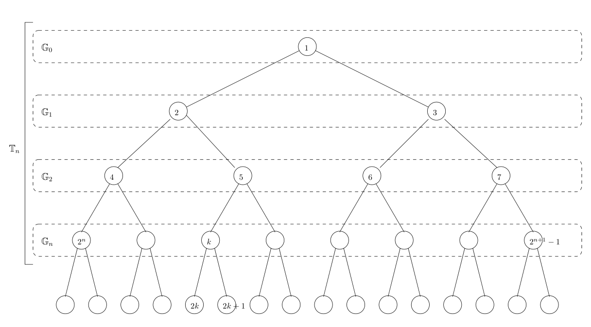
This assumption ensures the stability (non explosion) of the BAR process. As explained in the introduction, one can see this BAR process as a first-order autoregressive process on a binary tree, where each vertex represents an individual or cell, vertex 11 being the original ancestor, see Figure 2 for an illustration.
Refer to caption
Figure 2: The tree associated with the bifurcating auto-regressive process.

We use the same notation as in [3]. For all n≥1n\geq 1, denote the nn-th generation by 𝔾n={2n,2n+1,…,2n+1−1}\mathbb{G}_{n}=\{2^{n},2^{n}+1,\ldots,2^{n+1}-1\}. In particular, 𝔾0={1}\mathbb{G}_{0}=\{1\} is the initial generation, and 𝔾1={2,3}\mathbb{G}_{1}=\{2,3\} is the first generation of offspring from the first ancestor. Let 𝔾rk\mathbb{G}_{r_{k}} be the generation of individual kk, which means that rk=[log2⁡(k)]r_{k}=[\log_{2}(k)], where [x][x] denotes the largest integer less than or equal to xx. Recall that the two offspring of individual kk are labelled 2​k2k and 2​k+12k+1, or conversely, the mother of individual kk is [k/2][k/2]. More generally, the ancestors of individual kk are [k/2],[k/22],…,[k/2rk][k/2],[k/2^{2}],\ldots,\ [k/2^{r_{k}}]. Denote by 𝕋n=⋃ℓ=0n𝔾ℓ,\mathbb{T}_{n}=\bigcup_{\ell=0}^{n}\mathbb{G}_{\ell},the sub-tree of all individuals from the original individual up to the nn-th generation. Note that the cardinality |𝔾n||\mathbb{G}_{n}| of 𝔾n\mathbb{G}_{n} is 2n2^{n}, while that of 𝕋n\mathbb{T}_{n} is |𝕋n|=2n+1−1|\mathbb{T}_{n}|=2^{n+1}-1. Next, 𝕋\mathbb{T} denotes the complete tree, so to speak 𝕋=⋃n≥0𝔾n=⋃n≥0𝕋n=ℕ∗=ℕ\{0}\mathbb{T}=\bigcup_{n\geq 0}\mathbb{G}_{n}=\bigcup_{n\geq 0}\mathbb{T}_{n}=\mathbb{N}^{*}=\mathbb{N}\backslash\{0\}. Finally, we need to distinguish the individuals in 𝔾n\mathbb{G}_{n} and 𝕋n\mathbb{T}_{n} according to their type. Since we are dealing with the types even and odd, that we will also label 00 and 11, we set

𝔾n0=𝔾n∩(2​ℕ),𝔾n1=𝔾n∩(2​ℕ+1),𝕋n0=𝕋n∩(2​ℕ),\mathbb{G}_{n}^{0}=\mathbb{G}_{n}\cap(2\mathbb{N}),\quad\mathbb{G}_{n}^{1}=\mathbb{G}_{n}\cap(2\mathbb{N}+1),\quad\mathbb{T}_{n}^{0}=\mathbb{T}_{n}\cap(2\mathbb{N}),
𝕋n1=𝕋n∩(2ℕ+1),𝕋0=𝕋∩(2ℕ)and𝕋1=𝕋∩(2ℕ+1).\mathbb{T}_{n}^{1}=\mathbb{T}_{n}\cap(2\mathbb{N}+1),\quad\mathbb{T}^{0}=\mathbb{T}\cap(2\mathbb{N})\quad\text{and}\quad\mathbb{T}^{1}=\mathbb{T}\cap(2\mathbb{N}+1). (2.2)

We now state our assumptions on the noise sequence. Denote by 𝔽=(ℱn)\mathbb{F}=(\mathcal{F}_{n}) the natural filtration associated with the first-order BAR process, which means that ℱn\mathcal{F}_{n} is the σ\sigma-algebra generated by all individuals up to the nn-th generation, ℱn=σ⁡{Xk,k∈𝕋n}\mathcal{F}_{n}=\sigma\{X_{k},k\in\mathbb{T}_{n}\}. In all the sequel, we shall make use of the following moment and independence hypotheses.

(HN.1)

For all n≥0n\geq 0 and for all k∈𝔾n+1k\in\mathbb{G}_{n+1}, εk\varepsilon_{k} belongs to L8L^{8}. Moreover, there exist (σ2,τ4,κ8)∈(0,+∞)3(\sigma^{2},\tau^{4},\kappa^{8})\in(0,+\infty)^{3}, (|ρ′|,ν2,λ4)∈[0,1)3(|\rho^{\prime}|,\nu^{2},\lambda^{4})\in[0,1)^{3} such that :

  • •

    ∀n≥0​ and ​k∈𝔾n+1\forall n\geq 0\text{ and }k\in\mathbb{G}_{n+1},

    𝔼⁡[εk|ℱn]=0,𝔼⁡[εk2|ℱn]=σ2,𝔼⁡[εk4|ℱn]=τ4,𝔼⁡[εk8|ℱn]=κ8​a.s.\mathbb{E}[\varepsilon_{k}|\mathcal{F}_{n}]=0,\hskip 2.84544pt\mathbb{E}[\varepsilon_{k}^{2}|\mathcal{F}_{n}]=\sigma^{2},\hskip 2.84544pt\mathbb{E}[\varepsilon_{k}^{4}|\mathcal{F}_{n}]=\tau^{4},\hskip 2.84544pt\mathbb{E}[\varepsilon_{k}^{8}|\mathcal{F}_{n}]=\kappa^{8}\hskip 5.69046pt\text{a.s.}
  • •

    ∀n≥0∀k≠l∈𝔾n+1​ with ​[k/2]=[l/2]\forall n\geq 0\quad\forall k\neq l\in\mathbb{G}_{n+1}\text{ with }[k/2]=[l/2],

    𝔼⁡[εk​εl|ℱn]=ρ=ρ′​σ2,𝔼⁡[ε2​k2​ε2​k+12|ℱn]=ν2​τ4,𝔼⁡[ε2​k4​ε2​k+14|ℱn]=λ4​κ8​a.s.\hskip-51.21504pt\mathbb{E}[\varepsilon_{k}\varepsilon_{l}|\mathcal{F}_{n}]=\rho=\rho^{\prime}\sigma^{2},\hskip 2.84544pt\mathbb{E}[\varepsilon_{2k}^{2}\varepsilon_{2k+1}^{2}|\mathcal{F}_{n}]=\nu^{2}\tau^{4},\hskip 2.84544pt\mathbb{E}[\varepsilon_{2k}^{4}\varepsilon_{2k+1}^{4}|\mathcal{F}_{n}]=\lambda^{4}\kappa^{8}\hskip 5.69046pt\text{a.s.}
(HN.2)

For all n≥0n\geq 0 the random vectors {(ε2​k,ε2​k+1),k∈𝔾n}\{(\varepsilon_{2k},\varepsilon_{2k+1}),k\in\mathbb{G}_{n}\} are conditionally independent given ℱn\mathcal{F}_{n}.

2.2 Observation process

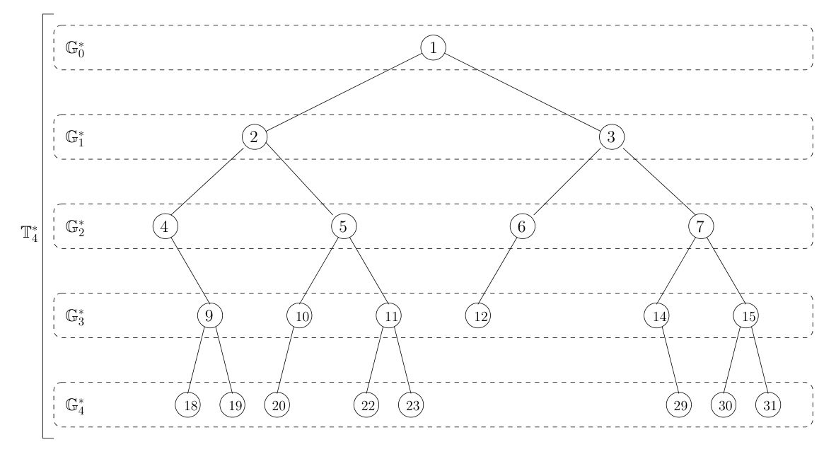
We now turn to the modeling of the observation process. The observation process is intended to encode if a datum is missing or not. The natural property it has thus to satisfy is the following: if the datum is missing for some individual, it is also missing for all its descendants. Indeed, the datum may be missing because of the death of the individual, or because the individual is the last of its lineage at the end of the data’s gathering, see Figure 3 for an example of partially observed tree.
Refer to caption
Figure 3: The tree associated with the observed data of the tree in Figure 1.

2.2.1 Definition of the observation process

Mathematically, we define the observation process, (δk)k∈𝕋(\delta_{k})_{k\in\mathbb{T}}, as follows. We set δ1=1\delta_{1}=1 and define recursively the sequence through the following equalities:

δ2​k=δk​ζk0andδ2​k+1=δk​ζk1,\delta_{2k}=\delta_{k}\zeta_{k}^{0}\quad\text{and}\quad\delta_{2k+1}=\delta_{k}\zeta_{k}^{1}, (2.3)

where (𝜻k=(ζk0,ζk1))(\boldsymbol{\zeta}_{k}=(\zeta_{k}^{0},\zeta_{k}^{1})) is a sequence of independent random vectors of {0,1}2\{0,1\}^{2}, ζki\zeta_{k}^{i} standing for the number (00 or 11) of descendants of type ii of individual kk. The sequences (𝜻k,k∈2​ℕ∗)(\boldsymbol{\zeta}_{k},k\in 2\mathbb{N}^{*}) and (𝜻k,k∈2​ℕ+1)(\boldsymbol{\zeta}_{k},k\in 2\mathbb{N}+1) are sequences of identically distributed random vectors. We specify the common laws of these two sequences using their generating functions, f(0)f^{(0)} and f(1)f^{(1)} respectively:

f(0)​(s0,s1)\displaystyle f^{(0)}(s_{0},s_{1}) =\displaystyle= p(0)​(0,0)+p(0)​(1,0)​s0+p(0)​(0,1)​s1+p(0)​(1,1)​s0​s1,\displaystyle p^{(0)}(0,0)+p^{(0)}(1,0)s_{0}+p^{(0)}(0,1)s_{1}+p^{(0)}(1,1)s_{0}s_{1},
f(1)​(s0,s1)\displaystyle f^{(1)}(s_{0},s_{1}) =\displaystyle= p(1)​(0,0)+p(1)​(1,0)​s0+p(1)​(0,1)​s1+p(1)​(1,1)​s0​s1,\displaystyle p^{(1)}(0,0)+p^{(1)}(1,0)s_{0}+p^{(1)}(0,1)s_{1}+p^{(1)}(1,1)s_{0}s_{1},

where p(i)​(j0,j1)p^{(i)}(j_{0},j_{1}) is the probability that an individual of type ii gives birth to j0j_{0} descendants of type 00, and j1j_{1} of type 11. The sequence (δk)(\delta_{k}) is thus completely defined. We also assume that the observation process is independent from the BAR process.

(HI)

The sequences (δk)(\delta_{k}) and (𝜻k)(\boldsymbol{\zeta}_{k}) are independent from the sequences (Xk)(X_{k}) and (εk)(\varepsilon_{k}).

Remark that, since both ζk0\zeta^{0}_{k} and ζk1\zeta^{1}_{k} take values in {0,1}\{0,1\} for all kk, the observation process (δk)(\delta_{k}) is itself taking values in {0,1}\{0,1\}. Finally, Equation (2.3) ensures that if δk=0\delta_{k}=0 for some k≥2k\geq 2, then for all its descendants jj, δj=0\delta_{j}=0. In relation with the observation process (δk)(\delta_{k}), we introduce two filtrations: 𝒵n=σ⁡{𝜻k,k∈𝕋n}\mathcal{Z}_{n}=\sigma\{\boldsymbol{\zeta}_{k},k\in\mathbb{T}_{n}\}, 𝒪n=σ⁡{δk,k∈𝕋n}\mathcal{O}_{n}=\sigma\{\delta_{k},k\in\mathbb{T}_{n}\}, and the sigma field 𝒪=σ⁡{δk,k∈𝕋}\mathcal{O}=\sigma\{\delta_{k},k\in\mathbb{T}\}. Notice that 𝒪n+1⊂𝒵n\mathcal{O}_{n+1}\subset\mathcal{Z}_{n}. We also define the sets of observed individuals as follows:

𝔾n∗={k∈𝔾n:δk=1}and𝕋n∗={k∈𝕋n:δk=1}.\mathbb{G}_{n}^{*}=\{k\in\mathbb{G}_{n}:\delta_{k}=1\}\quad\text{and}\quad\mathbb{T}_{n}^{*}=\{k\in\mathbb{T}_{n}:\delta_{k}=1\}.

Finally, let ℰ\mathcal{E} be the event corresponding to the cases when there are no individual left to observe. More precisely,

ℰ=⋃n≥1{|𝔾n∗|=0}.\mathcal{E}=\bigcup_{n\geq 1}\{|\mathbb{G}_{n}^{*}|=0\}. (2.4)

We will denote ℰ¯\overline{\mathcal{E}} the complementary set of ℰ\mathcal{E}.

2.2.2 Results on the observation process

Let us introduce some additional notation. For n≥1n\geq 1, we define the number of observed individuals among the n-th generation, distinguishing according to their types:

Zn0=|𝔾n∗∩2​ℕ|andZn1=|𝔾n∗∩(2​ℕ+1)|,Z_{n}^{0}=|\mathbb{G}_{n}^{*}\cap 2\mathbb{N}|\quad\text{and}\quad Z_{n}^{1}=|\mathbb{G}_{n}^{*}\cap(2\mathbb{N}+1)|, (2.5)

and we set, for all n≥1n\geq 1, 𝒁n=(Zn0,Zn1)\boldsymbol{Z}_{n}=(Z_{n}^{0},Z_{n}^{1}). Note that for i∈{0,1}i\in\{0,1\} and n≥1n\geq 1 one has

Zni=∑k∈𝔾n−1δ2​k+i.Z_{n}^{i}=\sum_{k\in\mathbb{G}_{n-1}}\delta_{2k+i}.

One has 𝔾0∗=𝔾0={1}\mathbb{G}_{0}^{*}=\mathbb{G}_{0}=\{1\}, but, even if 11 is odd, the individual whose lineage we study may as well be of type 00 as of type 11. Consequently, we will work with possibly two different initial laws: ℙ(⋅|𝒁0=𝒆i)\mathbb{P}(\cdot|\boldsymbol{Z}_{0}=\boldsymbol{e}_{i}), for i∈{0,1}i\in\{0,1\}, where 𝒆0=(1,0)\boldsymbol{e}_{0}=(1,0) and 𝒆1=(0,1)\boldsymbol{e}_{1}=(0,1). The process (𝒁n,n≥0)(\boldsymbol{Z}_{n},n\geq 0) is thus a two-type Galton-Watson process, and all the results we are giving in this section mainly come from [12]. Notice that the law of 𝜻k\boldsymbol{\zeta}_{k}, for even kk, is the law of reproduction of an individual of type 00, the first component of 𝜻k\boldsymbol{\zeta}_{k} giving the number of children of type 00, the second the number of children of type 11. The same holds for 𝜻k\boldsymbol{\zeta}_{k}, with odd kk, mutatis mutandis. This ensures the existence of moments of all order for these reproduction laws, and we can thus define the descendants matrix 𝑷\boldsymbol{P}

𝑷=(p00p01p10p11),\boldsymbol{P}=\left(\begin{array}[]{cc}p_{00}&p_{01}\\ p_{10}&p_{11}\end{array}\right),

where pi​0=p(i)​(1,0)+p(i)​(1,1)p_{i0}=p^{(i)}(1,0)+p^{(i)}(1,1) and pi​1=p(i)​(0,1)+p(i)​(1,1)p_{i1}=p^{(i)}(0,1)+p^{(i)}(1,1), for i∈{0,1}i\in\{0,1\}. The quantity pi​j=𝔼⁡[ζ2+ij]p_{ij}=\mathbb{E}[\zeta_{2+i}^{j}] is thus the expected number of descendants of type jj of an individual of type ii. We also introduce the variance of the laws of reproduction: σi​j2=𝔼⁡[(ζ2+ij−pi​j)2]\sigma_{ij}^{2}=\mathbb{E}[(\zeta_{2+i}^{j}-p_{ij})^{2}], for (i,j)∈{0,1}2(i,j)\in\{0,1\}^{2}. Note that σi​j2=pi​j​(1−pi​j)\sigma_{ij}^{2}=p_{ij}(1-p_{ij}). It is well-known (see e.g. Theorem 5.1 of [12]) that when all the entries of the matrix 𝑷\boldsymbol{P} are positive, 𝑷\boldsymbol{P} has a positive strictly dominant eigenvalue, denoted π\pi, which is also simple. We make the following main assumptions on the matrix 𝑷\boldsymbol{P}.

(HO)

All entries of the matrix 𝑷\boldsymbol{P} are positive: for all (i,j)∈{0,1}2(i,j)\in\{0,1\}^{2}, pi​j>0p_{ij}>0, and the dominant eigenvalue is greater than one: π>1\pi>1 .

Hence, still following Theorem 5.1 of [12], we know that there exist left and right eigenvectors for π\pi which are positive, in the sense that each component of the vector is positive. We call 𝒚=(y0,y1)t\boldsymbol{y}=(y^{0},y^{1})^{t} such a right eigenvector, and 𝒛=(z0,z1)\boldsymbol{z}=(z^{0},z^{1}) such a left one; without loss of generality, we choose 𝒛\boldsymbol{z} such that z0+z1=1z^{0}+z^{1}=1. Regarding the two-type Galton-Watson process (𝒁n)(\boldsymbol{Z}_{n}), π\pi plays the same role as the expected number of offspring, in the case of standard Galton-Watson processes. In particular, π\pi is related to the extinction of the process, where the set of extinction of (𝒁n)(\boldsymbol{Z}_{n}) is defined as ∪n≥1{𝒁n=(0,0)}\cup_{n\geq 1}\{\boldsymbol{Z}_{n}=(0,0)\}. Notice that {𝒁n=(0,0)}={Zn0+Zn1=0}={|𝔾n∗|=0}\{\boldsymbol{Z}_{n}=(0,0)\}=\{Z_{n}^{0}+Z_{n}^{1}=0\}=\{|\mathbb{G}_{n}^{*}|=0\}, so that this set coincides with ℰ\mathcal{E}, defined by Eq. (2.4). Now let 𝒒=(q0,q1)\boldsymbol{q}=(q^{0},q^{1}), where, for i∈{0,1}i\in\{0,1\},

qi=ℙ⁡(ℰ|𝒁0=𝒆i).q^{i}=\mathbb{P}(\mathcal{E}|\boldsymbol{Z}_{0}=\boldsymbol{e}_{i}).

The probability qiq^{i} is thus the extinction probability if initially there is one individual of type ii. These two probabilities allow to compute the extinction probability under any initial distribution, since ℙ⁡(ℰ)=𝔼⁡[(q0)Z00​(q1)Z01]\mathbb{P}(\mathcal{E})=\mathbb{E}[(q^{0})^{Z_{0}^{0}}(q^{1})^{Z_{0}^{1}}], thanks to the branching property. Hypothesis (HO) means that the Galton-Watson process (𝒁n)(\boldsymbol{Z}_{n}) is super-critical, and ensures that 0≤qi<10\leq q^{i}<1, for both i=0i=0 and i=1i=1. This immediately yields

ℙ⁡(ℰ)<1.\mathbb{P}(\mathcal{E})<1. (2.6)

Under that condition, we also have the existence of a non-negative random variable WW such that for any initial distribution of 𝒁0\boldsymbol{Z}_{0}

limn→+∞𝒁nπn=limn→+∞π−1πn+1−1​∑ℓ=0n𝒁ℓ=W​𝒛a.s..\lim_{n\rightarrow+\infty}\frac{\boldsymbol{Z}_{n}}{\pi^{n}}=\lim_{n\rightarrow+\infty}\frac{\pi-1}{\pi^{n+1}-1}\sum_{\ell=0}^{n}\boldsymbol{Z}_{\ell}=W\boldsymbol{z}\quad\text{a.s.}. (2.7)

It is well-known that {W=0}=ℰ\{W=0\}=\mathcal{E} a.s., so that the set {W>0}\{W>0\} can be viewed as the set of non-extinction ℰ¯\overline{\mathcal{E}} of (𝒁n)(\boldsymbol{Z}_{n}), up to a negligible set. These results give the asymptotic behavior of the number of observed individuals, since |𝔾n∗|=Zn0+Zn1|\mathbb{G}^{*}_{n}|=Z_{n}^{0}+Z_{n}^{1}, and |𝕋n∗|=∑ℓ=0n(Zℓ0+Zℓ1CLOSE|\mathbb{T}^{*}_{n}|=\sum_{\ell=0}^{n}(Z_{\ell}^{0}+Z_{\ell}^{1}):

limn→+∞|𝔾n∗|πn=limn→+∞π−1πn+1−1​|𝕋n∗|=Wa.s.\lim_{n\rightarrow+\infty}\frac{|\mathbb{G}^{*}_{n}|}{\pi^{n}}=\lim_{n\rightarrow+\infty}\frac{\pi-1}{\pi^{n+1}-1}|\mathbb{T}^{*}_{n}|=W\hskip 14.22636pt\text{a.s.}

Roughly speaking, this means that πn\pi^{n} is a deterministic equivalent of |𝕋n∗||\mathbb{T}^{*}_{n}| and Eq. (2.7) implies that ziz^{i} is the asymptotic proportion of cells of type ii in a given generation. We will thus very often replace |𝕋n∗||\mathbb{T}^{*}_{n}| by πn\pi^{n} for computations, and the next lemma will be used frequently to replace πn\pi^{n} by |𝕋n∗||\mathbb{T}^{*}_{n}|.

Lemma 2.1

Under assumption (HO), we have

limn→+∞𝟙{|𝔾n∗|>0}πn|𝕋n∗|=π−1π1W𝟙ℰ¯a.s.\lim_{n\rightarrow+\infty}\mathbbm{1}_{\{|\mathbb{G}_{n}^{*}|>0\}}\frac{\pi^{n}}{|\mathbb{T}^{*}_{n}|}=\frac{\pi-1}{\pi}\frac{1}{W}\mathbbm{1}_{\overline{\mathcal{E}}}\quad\text{a.s.}

2.3 Joint model

The model under study in this paper is therefore the observed BAR process defined by

{δ2​k​X2​k=δ2​k(aCLOSE+b​Xk+OPENε2​k),δ2​k+1​X2​k+1=δ2​k+1(cCLOSE+d​Xk+OPENε2​k+1).\left\{\begin{array}[]{rccccccl}\delta_{2k}X_{2k}&=&\delta_{2k}&(a&+&bX_{k}&+&\varepsilon_{2k}),\\ \delta_{2k+1}X_{2k+1}&=&\delta_{2k+1}&(c&+&dX_{k}&+&\varepsilon_{2k+1}).\end{array}\right.

The aim of this paper is to study the sharp asymptotic properties of the least-squares estimators of the parameters (a,b,c,d)(a,b,c,d) and the variance matrix of the noise process.

3 Least-squares estimation

Our goal is to estimate 𝜽=(a,b,c,d)t{\boldsymbol{\theta}}=(a,b,c,d)^{t} from the observed individuals up to the nn-th generation, that is the observed sub-tree 𝕋n∗\mathbb{T}_{n}^{*}.

3.1 Definition of the estimators

We propose to make use of the standard least-squares (LS) estimator 𝜽^n\widehat{{\boldsymbol{\theta}}}_{n} which minimizes

Δn​(𝜽)=∑k∈𝕋n−1δ2​k​(X2​k−a−b​Xk)2+δ2​k+1​(X2​k+1−c−d​Xk)2.\Delta_{n}(\boldsymbol{\theta})=\sum_{k\in\mathbb{T}_{n-1}}\delta_{2k}(X_{2k}-a-bX_{k})^{2}+\delta_{2k+1}(X_{2k+1}-c-dX_{k})^{2}.

Consequently, we obviously have for all n≥1n\geq 1

(𝜽^n)=(a^nb^nc^nd^n)=𝚺n−1−1​∑k∈𝕋n−1(δ2​k​X2​kδ2​k​Xk​X2​kδ2​k+1​X2​k+1δ2​k+1​Xk​X2​k+1),(\widehat{\boldsymbol{\theta}}_{n})=\left(\begin{array}[]{c}\widehat{a}_{n}\\ \widehat{b}_{n}\\ \widehat{c}_{n}\\ \widehat{d}_{n}\end{array}\right)=\boldsymbol{\Sigma}_{n-1}^{-1}\sum_{k\in\mathbb{T}_{n-1}}\left(\begin{array}[]{c}\delta_{2k}X_{2k}\\ \delta_{2k}X_{k}X_{2k}\\ \delta_{2k+1}X_{2k+1}\\ \delta_{2k+1}X_{k}X_{2k+1}\end{array}\right), (3.1)

where, for all n≥0n\geq 0,

𝚺n=(𝑺n000𝑺n1),and𝑺ni=∑k∈𝕋nδ2​k+i​(1XkXkXk2),\boldsymbol{\Sigma}_{n}=\left(\begin{array}[]{cc}\boldsymbol{S}^{0}_{n}&0\\ 0&\boldsymbol{S}^{1}_{n}\end{array}\right),\quad\textrm{and}\quad\boldsymbol{S}^{i}_{n}=\sum_{k\in\mathbb{T}_{n}}\delta_{2k+i}\left(\begin{array}[]{cc}1&X_{k}\\ X_{k}&X^{2}_{k}\end{array}\right),

for i∈{0,1}i\in\{0,1\}. In order to avoid intricate invertibility assumption, we shall assume, without loss of generality, that for all n≥0n\geq 0, 𝚺n\boldsymbol{\Sigma}_{n} is invertible. Otherwise, we only have to add the identity matrix 𝐈4\boldsymbol{\mathrm{I}}_{4} to 𝚺n\boldsymbol{\Sigma}_{n}, as Proposition 4.2 states that the normalized limit of 𝚺n\boldsymbol{\Sigma}_{n} is positive definite.

Remark 3.1

Note that when all data are observed, that is when all δk\delta_{k} equal 11, this is simply the least squares estimator described in the previous literature. However, one must be careful here with the indices in the normalizing matrix, as there are now two different matrices 𝐒n0\boldsymbol{S}^{0}_{n} and 𝐒n1\boldsymbol{S}^{1}_{n}, while there was only one in the fully observed problem. The intuitive way to deal with missing data would be to restrict the sums to the observed data only. Note that our estimator is more complex as it involves sums depending on the absence or presence of even- or odd-type daughters of the available data.

We now turn to the estimation of the parameters σ2\sigma^{2} and ρ\rho. We propose to estimate the conditional variance σ2\sigma^{2} and the conditional covariance ρ\rho by

σ^n2=1|𝕋n∗|​∑k∈𝕋n−1∗(ε^2​k2+ε^2​k+12),ρ^n=1|𝕋n−1∗01|​∑k∈𝕋n−1ε^2​k​ε^2​k+1,\widehat{\sigma}^{2}_{n}=\frac{1}{|\mathbb{T}_{n}^{*}|}\sum_{k\in\mathbb{T}^{*}_{n-1}}(\widehat{\varepsilon}_{2k}^{2}+\widehat{\varepsilon}_{2k+1}^{2}),\quad\widehat{\rho}_{n}=\frac{1}{|\mathbb{T}_{n-1}^{*01}|}\sum_{k\in\mathbb{T}_{n-1}}\widehat{\varepsilon}_{2k}\widehat{\varepsilon}_{2k+1},

where for all k∈𝔾nk\in\mathbb{G}_{n},

{ε^2​k=δ2​k​(X2​kCLOSE−a^n−OPENb^n​Xk),ε^2​k+1=δ2​k+1​(X2​k+1CLOSE−c^n−OPENd^n​Xk).,\left\{\begin{array}[]{lcrclcl}\widehat{\varepsilon}_{2k}&=&\delta_{2k}(X_{2k}&-&\widehat{a}_{n}&-&\widehat{b}_{n}X_{k}),\\ \widehat{\varepsilon}_{2k+1}&=&\delta_{2k+1}(X_{2k+1}&-&\widehat{c}_{n}&-&\widehat{d}_{n}X_{k}).\end{array}\right.,

and

𝕋n∗01={k∈𝕋n:δ2​k​δ2​k+1=1},\mathbb{T}_{n}^{*01}=\{k\in\mathbb{T}_{n}:\delta_{2k}\delta_{2k+1}=1\},

so to speak 𝕋n−1∗01\mathbb{T}_{n-1}^{*01} is the set of the cells of the tree 𝕋n−1\mathbb{T}_{n-1} which have exactly two offspring.

3.2 Main results

We can now state the sharp convergence results we obtain for the estimators above. We introduce additional notation. For i∈{0,1}i\in\{0,1\}, let us denote :

𝑳i=(π​zihihiki)𝑳0,1=(p¯​(1,1)h0,1h0,1k0,1)\boldsymbol{L}^{i}=\left(\begin{array}[]{cc}\pi z^{i}&h^{i}\\ h^{i}&k^{i}\end{array}\right)\qquad\qquad\boldsymbol{L}^{0,1}=\left(\begin{array}[]{cc}\bar{p}(1,1)&h^{0,1}\\ h^{0,1}&k^{0,1}\end{array}\right)

where 𝒛=(z0,z1)\boldsymbol{z}=(z^{0},z^{1}) is the left eigenvector for the dominant eigenvalue π\pi of the descendants matrix 𝑷\boldsymbol{P} introduced in section 2.2.2, hih^{i}, kik^{i} are defined in Propositions 6.3 and 6.5 and the four terms of L0,1L^{0,1} defined in Proposition 6.6. We also define the 4×44\times 4 matrices

𝚺=(𝑳000𝑳1),and𝚪=(σ2​𝑳0ρ​𝑳0,1ρ​𝑳0,1σ2​𝑳1).\boldsymbol{\Sigma}=\left(\begin{array}[]{cc}\boldsymbol{L}^{0}&0\\ 0&\boldsymbol{L}^{1}\end{array}\right),\quad\textrm{and}\quad\boldsymbol{\Gamma}=\left(\begin{array}[]{cc}\sigma^{2}\boldsymbol{L}^{0}&\rho\boldsymbol{L}^{0,1}\\ \rho\boldsymbol{L}^{0,1}&\sigma^{2}\boldsymbol{L}^{1}\end{array}\right). (3.2)

Our first result deals with the strong consistency of the LS estimator 𝜽^n\widehat{\boldsymbol{\theta}}_{n}.

Theorem 3.2

Under assumptions (HN.1), (HN.2), (HO) and (HI), 𝛉^n\widehat{\boldsymbol{\theta}}_{n} converges to 𝛉\boldsymbol{\theta} almost surely on ℰ¯\overline{\mathcal{E}} with the rate of convergence

𝟙{|𝔾n∗|>0}∥𝜽^n−𝜽∥2=𝒪(log⁡|𝕋n−1∗||𝕋n−1∗|)𝟙ℰ¯a.s.\mathbbm{1}_{\{|\mathbb{G}_{n}^{*}|>0\}}\|\widehat{\boldsymbol{\theta}}_{n}-\boldsymbol{\theta}\|^{2}=\mathcal{O}\left(\frac{\log|\mathbb{T}_{n-1}^{*}|}{|\mathbb{T}_{n-1}^{*}|}\right)\mathbbm{1}_{\overline{\mathcal{E}}}\hskip 28.45274pt\text{a.s.} (3.3)

In addition, we also have the quadratic strong law

limn→∞𝟙{|𝔾n∗|>0}1n∑ℓ=1n|𝕋ℓ−1∗|(𝜽^ℓ−𝜽)t𝚺(𝜽^ℓ−𝜽)=4π−1πσ2𝟙ℰ¯a.s.\lim_{n\rightarrow\infty}\mathbbm{1}_{\{|\mathbb{G}_{n}^{*}|>0\}}\frac{1}{n}\sum_{\ell=1}^{n}|\mathbb{T}_{\ell-1}^{*}|(\widehat{\boldsymbol{\theta}}_{\ell}-\boldsymbol{\theta})^{t}\boldsymbol{\Sigma}(\widehat{\boldsymbol{\theta}}_{\ell}-\boldsymbol{\theta})=4\frac{\pi-1}{\pi}\sigma^{2}\mathbbm{1}_{\overline{\mathcal{E}}}\hskip 28.45274pt\text{a.s.} (3.4)

Our second result is devoted to the almost sure asymptotic properties of the variance and covariance estimators σ^n2\widehat{\sigma}^{2}_{n} and ρ^n\widehat{\rho}_{n}. Let

σn2=1|𝕋n∗|​∑k∈𝕋n−1∗(δ2​k​ε2​k2+δ2​k+1​ε2​k+12),ρn=1|𝕋n−1∗01|​∑k∈𝕋n−1∗δ2​k​ε2​k​δ2​k+1​ε2​k+1.\sigma^{2}_{n}=\frac{1}{|\mathbb{T}_{n}^{*}|}\sum_{k\in\mathbb{T}^{*}_{n-1}}\!\!\!\!(\delta_{2k}{\varepsilon}_{2k}^{2}+\delta_{2k+1}{\varepsilon}_{2k+1}^{2}),\quad{\rho}_{n}=\frac{1}{|\mathbb{T}_{n-1}^{*01}|}\sum_{k\in\mathbb{T}^{*}_{n-1}}\!\!\!\!{\delta_{2k}\varepsilon}_{2k}\delta_{2k+1}{\varepsilon}_{2k+1}.
Theorem 3.3

Under assumptions (HN.1), (HN.2), (HO) and (HI), σ^n2\widehat{\sigma}^{2}_{n} converges almost surely to σ2\sigma^{2} on ℰ¯\overline{\mathcal{E}}. More precisely, one has

limn→∞𝟙{|𝔾n∗|>0}1n∑k∈𝕋n−1∑i=01δ2​k+i(ε^2​k+i−ε2​k+i)2=4(π−1)σ2𝟙ℰ¯a.s.\lim_{n\rightarrow\infty}\mathbbm{1}_{\{|\mathbb{G}_{n}^{*}|>0\}}\frac{1}{n}\sum_{k\in\mathbb{T}_{n-1}}\sum_{i=0}^{1}\delta_{2k+i}(\widehat{\varepsilon}_{2k+i}-\varepsilon_{2k+i})^{2}={4}{(\pi-1)}\sigma^{2}\mathbbm{1}_{\overline{\mathcal{E}}}\hskip 5.69046pt\text{a.s.} (3.5)
limn→∞𝟙{|𝔾n∗|>0}|𝕋n∗|n(σ^n2−σn2)=4(π−1)σ2𝟙ℰ¯a.s.\lim_{n\rightarrow\infty}\mathbbm{1}_{\{|\mathbb{G}_{n}^{*}|>0\}}\frac{|\mathbb{T}_{n}^{*}|}{n}(\widehat{\sigma}^{2}_{n}-\sigma_{n}^{2})={4}{(\pi-1)}\sigma^{2}\mathbbm{1}_{\overline{\mathcal{E}}}\hskip 28.45274pt\text{a.s.} (3.6)

In addition, ρ^n\widehat{\rho}_{n} converges almost surely to ρ\rho on ℰ¯\overline{\mathcal{E}} and one has

limn→∞𝟙{|𝔾n∗|>0}\displaystyle\lim_{n\rightarrow\infty}\mathbbm{1}_{\{|\mathbb{G}_{n}^{*}|>0\}} 1n​∑k∈𝕋n−1δ2​k​(ε^2​k−ε2​k)​δ2​k+1​(ε^2​k+1−ε2​k+1)\displaystyle\frac{1}{n}\sum_{k\in\mathbb{T}_{n-1}}\delta_{2k}(\widehat{\varepsilon}_{2k}-\varepsilon_{2k})\delta_{2k+1}(\widehat{\varepsilon}_{2k+1}-\varepsilon_{2k+1})
=4ρπ−1πtr((𝑳1)−1/2𝑳0,1(𝑳0)−1/2)𝟙ℰ¯a.s.\displaystyle=4\rho\frac{\pi-1}{\pi}tr\big((\boldsymbol{L}^{1})^{-1/2}\boldsymbol{L}^{0,1}(\boldsymbol{L}^{0})^{-1/2}\big)\mathbbm{1}_{\overline{\mathcal{E}}}\hskip 14.22636pt\text{a.s.} (3.7)
limn→∞𝟙{|𝔾n∗|>0}|𝕋n∗|n(ρ^n−ρn)=ρπ−1p¯​(1,1)tr((𝑳1)−1(𝑳0,1)2(𝑳0)−1)𝟙ℰ¯a.s.\lim_{n\rightarrow\infty}\mathbbm{1}_{\{|\mathbb{G}_{n}^{*}|>0\}}\frac{|\mathbb{T}_{n}^{*}|}{n}(\widehat{\rho}_{n}-\rho_{n})=\rho\frac{\pi-1}{\bar{p}(1,1)}tr\big((\boldsymbol{L}^{1})^{-1}(\boldsymbol{L}^{0,1})^{2}(\boldsymbol{L}^{0})^{-1}\big)\mathbbm{1}_{\overline{\mathcal{E}}}\hskip 14.22636pt\text{a.s.} (3.8)

Our third result concerns the asymptotic normality for all our estimators 𝜽^n\widehat{\boldsymbol{\theta}}_{n}, σ^n2\widehat{\sigma}^{2}_{n} and ρ^n\widehat{\rho}_{n} given the non-extinction of the underlying Galton-Watson process. For this, using the fact that ℙ⁡(ℰ¯)≠0\mathbb{P}(\overline{\mathcal{E}})\neq 0 thanks to Eq. (2.6), we define the probability ℙℰ¯\mathbb{P}_{\overline{\mathcal{E}}} by

ℙℰ¯​(A)=ℙ⁡(A∩ℰ¯)ℙ⁡(ℰ¯) for all ​A∈𝒜.\mathbb{P}_{\overline{\mathcal{E}}}(A)=\frac{\mathbb{P}(A\cap\overline{\mathcal{E}})}{\mathbb{P}(\overline{\mathcal{E}})}\qquad\text{ for all }A\in{\cal A}.
Theorem 3.4

Under assumptions (HN.1), (HN.2), (HO) and (HI), we have the central limit theorem

|𝕋n−1∗|​(𝜽^n−𝜽)⟶ℒ𝒩⁡(0,𝚺−1​𝚪​𝚺−1)on ​(ℰ¯,ℙℰ¯).\sqrt{|\mathbb{T}^{*}_{n-1}|}(\widehat{\boldsymbol{\theta}}_{n}-\boldsymbol{\theta})\mathrel{\mathop{\kern 0.0pt\longrightarrow}\limits^{\mathcal{L}}}\mathcal{N}(0,\boldsymbol{\Sigma}^{-1}\boldsymbol{\Gamma}\boldsymbol{\Sigma}^{-1})\quad\text{on }\ ({\overline{\mathcal{E}}},\mathbb{P}_{\overline{\mathcal{E}}}). (3.9)

In addition, we also have

|𝕋n∗|​(σ^n2−σ2)⟶ℒ𝒩⁡(0,π⁡(τ4−σ4)+2​p¯​(1,1)​(ν2​τ4−σ4)π)on ​(ℰ¯,ℙℰ¯),\sqrt{|\mathbb{T}^{*}_{n}|}(\widehat{\sigma}^{2}_{n}-{\sigma}^{2})\mathrel{\mathop{\kern 0.0pt\longrightarrow}\limits^{\mathcal{L}}}\mathcal{N}\Bigl(0,\frac{\pi(\tau^{4}-\sigma^{4})+2\bar{p}(1,1)(\nu^{2}\tau^{4}-\sigma^{4})}{\pi}\Bigr)\quad\text{on }\ ({\overline{\mathcal{E}}},\mathbb{P}_{\overline{\mathcal{E}}}), (3.10)

where p¯​(1,1)\bar{p}(1,1) is defined in Eq. (6.6) and

|𝕋n−1∗01|​(ρ^n−ρ)⟶ℒ𝒩⁡(0,ν2​τ4−ρ2)on ​(ℰ¯,ℙℰ¯).\sqrt{|\mathbb{T}^{*01}_{n-1}|}(\widehat{\rho}_{n}-{\rho})\mathrel{\mathop{\kern 0.0pt\longrightarrow}\limits^{\mathcal{L}}}\mathcal{N}(0,{\nu^{2}\tau^{4}-\rho^{2}})\quad\text{on }\ ({\overline{\mathcal{E}}},\mathbb{P}_{\overline{\mathcal{E}}}). (3.11)

The proof of our main results is going to be detailed in the next sections. It is based on martingale properties, and we will exhibit our main martingale (𝑴n)(\boldsymbol{M}_{n}) in Section 4. Sections 5 to 7 are devoted proving to the sharp asymptotic properties of (𝑴n)(\boldsymbol{M}_{n}). Finally, in Section 8 we prove our main results. Before turning to the definition of the martingale (𝑴n)(\boldsymbol{M}_{n}), we present a short application of our estimation procedure on data.

3.3 Results on real data

The biological issue addressed by Stewart et al. in [15] is aging in the single cell organism Escherichia coli, see also [7] for further biological details. E. coli is a rod-shaped bacterium that reproduces by dividing in the middle. Each cell has thus a new end (or pole), and an older one. The cell that inherits the old pole of its mother is called the old pole cell, the cell that inherits the new pole of its mother is called the new pole cell. Therefore, each cell has a type: old pole (even) or new pole (odd) cell, inducing asymmetry in the cell division.

Stewart et al. filmed colonies of dividing cells, determining the complete lineage and the growth rate of each cell. Their statistical study of the averaged genealogy and pair-wise comparison of sister cells showed that the old pole cells exhibit cumulatively slowed growth, less offspring biomass production and an increased probability of death. Note that their test assumes independence between the averaged pairs of sister cells which is not verified in the lineage.

Another analysis was proposed in [9]. They model the growth rate by a Markovian bifurcating process, allowing single-experiment statistical analysis instead of averaging all the genealogical trees. Asymptotic properties of a more general asymmetric Markovian bifurcating autoregressive process are then investigated in [8], where a Wald’s type test is rigorously constructed to study the asymmetry of the process. These results cannot be compared to ours because this model does not take into account the possibly missing data from the genealogies, and it is not clear how the author manages them, as not a single tree from the data of [15] is complete. In [5], the authors take missing data into account but, contrary to our approach, they allow different sets of parameters for cells with two, one or no offspring, making the direct comparison with our estimator again impossible.

We have applied our methodology on the set of data penna-2002-10-04-4 from the experiments of [15]. It is the largest data set of the experiment. It contains 663 cells up to generation 9 (note that there would be 1023 cells in a full tree up to generation 9). In particular, we have performed

  • •

    point estimation of the vector 𝜽\boldsymbol{\theta},

  • •

    interval estimation for the coefficients (a,b,c,d)(a,b,c,d),

  • •

    Wald’s type symmetry tests for the entries of 𝜽^n\widehat{\boldsymbol{\theta}}_{n}.

parameter aa cc
estimation 0.03627 0.03058
C.I. [0.03276;0.03979][0.03276;0.03979] [0.02696;0.03420][0.02696;0.03420]
parameter b d
estimation 0.02662 0.17055
C.I. [−0.06866;0.12191][-0.06866;0.12191] [0.07247;0.26863][0.07247;0.26863]
Table 1: Estimation on the data set penna-2002-10-04-4

Table 1 gives the estimation 𝜽^9\widehat{\boldsymbol{\theta}}_{9} of 𝜽^\widehat{\boldsymbol{\theta}} with the 95% Confidence Interval (C.I.) of each coefficient. The variance given by the CLT for 𝜽\boldsymbol{\theta} in Eq. (3.9), is approximated by 𝚺n−1​𝚪n​𝚺n−1\boldsymbol{\Sigma}^{-1}_{n}\boldsymbol{\Gamma}_{n}\boldsymbol{\Sigma}^{-1}_{n} thanks to the convergence given in Corollary 4.3. The confidence intervals of bb and dd show that the non explosion assumption (|b|<1|b|<1 and |d|<1|d|<1) is satisfied. Some empirical computation on the process (δk)(\delta_{k}) gives the following estimation for the highest eigenvalue of the Galton-Watson process : π^=1.35669\hat{\pi}=1.35669 (with confidence interval [1.27979,1.43361][1.27979,1.43361], see [14]), also satisfying the super-criticality assumption. Wald tests of comparison between the coefficients of 𝜽\boldsymbol{\theta} have been deduced of the CLT. The null hypotheses (a,b)=(c,d)(a,b)=(c,d) (resp. a=ca=c, b=db=d) are rejected with p-values p= 0.0211 (resp. p= 0.0158 and p=0.0244). Hence on this data set the cell division is indeed statistically asymmetric.

4 Martingale approach

To establish all the asymptotic properties of our estimators, we shall make use of a martingale approach, similar to [3]. However, their results cannot be used in our framework, since the randomness comes now not only from the state process, but also from the time space (genealogy). These two mixed randomness sources require careful choice between various filtrations, and stronger moment assumptions on the driven noise of the BAR process. For all n≥1n\geq 1, denote

𝑴n=∑k∈𝕋n−1(δ2​k​ε2​k,δ2​k​Xk​ε2​k,δ2​k+1​ε2​k+1,δ2​k+1​Xk​ε2​k+1)t.\boldsymbol{M}_{n}=\sum_{k\in\mathbb{T}_{n-1}}\left(\delta_{2k}\varepsilon_{2k},\ \delta_{2k}X_{k}\varepsilon_{2k},\ \delta_{2k+1}\varepsilon_{2k+1},\ \delta_{2k+1}X_{k}\varepsilon_{2k+1}\right)^{t}.

Thus, for all n≥2n\geq 2, we readily deduce from Equations (3.1) and (2.1) that

𝜽^n−𝜽=𝚺n−1−1​∑k∈𝕋n−1(δ2​k​ε2​kδ2​k​Xk​ε2​kδ2​k+1​ε2​k+1δ2​k+1​Xk​ε2​k+1)=𝚺n−1−1​𝑴n.\widehat{\boldsymbol{\theta}}_{n}-\boldsymbol{\theta}=\boldsymbol{\Sigma}^{-1}_{n-1}\sum_{k\in\mathbb{T}_{n-1}}\left(\begin{array}[]{cccc}\delta_{2k}\varepsilon_{2k}\\ \delta_{2k}X_{k}\varepsilon_{2k}\\ \delta_{2k+1}\varepsilon_{2k+1}\\ \delta_{2k+1}X_{k}\varepsilon_{2k+1}\end{array}\right)=\boldsymbol{\Sigma}^{-1}_{n-1}\boldsymbol{M}_{n}. (4.1)

The key point of our approach is that (𝑴n)(\boldsymbol{M}_{n}) is a martingale for a well chosen filtration.

4.1 Martingale property

Recall that 𝒪=σ⁡{δk,k∈𝕋}\mathcal{O}=\sigma\{\delta_{k},k\in\mathbb{T}\} is the σ\sigma-field generated by the observation process. We shall assume that all the history of the process (δk)(\delta_{k}) is known at time 00 and use the filtration 𝔽𝒪=(ℱn𝒪)\mathbb{F}^{\mathcal{O}}=(\mathcal{F}^{\mathcal{O}}_{n}) defined for all nn by

ℱn𝒪=𝒪∨σ⁡{δk​Xk,k∈𝕋n}=𝒪∨σ⁡{Xk,k∈𝕋n∗},\mathcal{F}^{\mathcal{O}}_{n}=\mathcal{O}\vee\sigma\{\delta_{k}X_{k},k\in\mathbb{T}_{n}\}=\mathcal{O}\vee\sigma\{X_{k},k\in\mathbb{T}_{n}^{*}\},

where ℱ∨𝒢\mathcal{F}\vee\mathcal{G} denotes the σ\sigma-field generated by both ℱ\mathcal{F} and 𝒢\mathcal{G}. Note that for all nn, ℱn𝒪\mathcal{F}^{\mathcal{O}}_{n} is a sub σ\sigma-field of 𝒪∨ℱn\mathcal{O}\vee\mathcal{F}_{n}.

Proposition 4.1

Under assumptions (HN.1), (HN.2) and (HI), the process (𝐌n)(\boldsymbol{M}_{n}) is a square integrable 𝔽𝒪\mathbb{F}^{\mathcal{O}}-martingale with increasing process given, for all n≥1n\geq 1, by

<𝑴>n=𝚪n−1=(σ2​𝑺n−10ρ​𝑺n−10,1ρ​𝑺n−10,1σ2​𝑺n−11),<\boldsymbol{M}>_{n}=\boldsymbol{\Gamma}_{n-1}=\left(\begin{array}[]{cc}\sigma^{2}\boldsymbol{S}^{0}_{n-1}&\rho\boldsymbol{S}^{0,1}_{n-1}\\ \rho\boldsymbol{S}^{0,1}_{n-1}&\sigma^{2}\boldsymbol{S}^{1}_{n-1}\end{array}\right),

where 𝐒n0\boldsymbol{S}^{0}_{n} and 𝐒n1\boldsymbol{S}^{1}_{n} are defined in section 3.1 and

𝑺n0,1=∑k∈𝕋nδ2​k​δ2​k+1​(1XkXkXk2).\boldsymbol{S}^{0,1}_{n}=\sum_{k\in\mathbb{T}_{n}}\delta_{2k}\delta_{2k+1}\left(\begin{array}[]{cc}1&X_{k}\\ X_{k}&X^{2}_{k}\end{array}\right).

Proof : First, notice that for all n≥1n\geq 1, one has

Δ​𝑴n=𝑴n−𝑴n−1=∑k∈𝔾n−1(δ2​k​ε2​kδ2​k​Xk​ε2​kδ2​k+1​ε2​k+1δ2​k+1​Xk​ε2​k+1).\Delta\boldsymbol{M}_{n}=\boldsymbol{M}_{n}-\boldsymbol{M}_{n-1}=\sum_{k\in\mathbb{G}_{n-1}}\left(\begin{array}[]{cccc}\delta_{2k}\varepsilon_{2k}\\ \delta_{2k}X_{k}\varepsilon_{2k}\\ \delta_{2k+1}\varepsilon_{2k+1}\\ \delta_{2k+1}X_{k}\varepsilon_{2k+1}\end{array}\right).

Now, we use the fact that for all nn, ℱn𝒪\mathcal{F}^{\mathcal{O}}_{n} is a sub-σ\sigma field of 𝒪∨ℱn\mathcal{O}\vee\mathcal{F}_{n}, the independence between 𝒪\mathcal{O} and ℱn\mathcal{F}_{n} under assumption (HI) and the moment hypothesis (HN.1) to obtain

𝔼⁡[δ2​k​ε2​k|ℱn−1𝒪]\displaystyle\mathbb{E}[\delta_{2k}\varepsilon_{2k}\ |\ \mathcal{F}^{\mathcal{O}}_{n-1}] =\displaystyle= δ2​k​𝔼​[𝔼⁡[ε2​k|𝒪∨ℱn−1]|ℱn−1𝒪]\displaystyle\delta_{2k}\mathbb{E}\big[\mathbb{E}[\varepsilon_{2k}\ |\ \mathcal{O}\vee\mathcal{F}_{n-1}]\ |\ \mathcal{F}^{\mathcal{O}}_{n-1}\big]
=\displaystyle= δ2​k​𝔼​[𝔼⁡[ε2​k|ℱn−1]|ℱn−1𝒪]= 0.\displaystyle\delta_{2k}\mathbb{E}\big[\mathbb{E}[\varepsilon_{2k}\ |\ \mathcal{F}_{n-1}]\ |\ \mathcal{F}^{\mathcal{O}}_{n-1}\big]\ =\ 0.

We obtain similar results for the other entries of Δ​𝑴n\Delta\boldsymbol{M}_{n} as δ2​k+1\delta_{2k+1} and XkX_{k} are also ℱn−1𝒪\mathcal{F}_{n-1}^{\mathcal{O}}-measurable. Hence, (𝑴n)(\boldsymbol{M}_{n}) is a 𝔽𝒪\mathbb{F}^{\mathcal{O}}-martingale. It is clearly square integrable from assumption (HN.1). The same measurability arguments together with assumption (HN.2) yield

𝔼⁡[Δ​𝑴n​(Δ​𝑴n)t|ℱn−1𝒪]\displaystyle\mathbb{E}[\Delta\boldsymbol{M}_{n}(\Delta\boldsymbol{M}_{n})^{t}\ |\ \mathcal{F}^{\mathcal{O}}_{n-1}]
=\displaystyle= ∑k∈𝔾n−1(σ2​δ2​kσ2​δ2​k​Xkρ​δ2​k​δ2​k+1ρ​δ2​k​δ2​k+1​Xkσ2​δ2​k​Xkσ2​δ2​k​Xk2ρ​δ2​k​δ2​k+1​Xkρ​δ2​k​δ2​k+1​Xk2ρ​δ2​k​δ2​k+1ρ​δ2​k​δ2​k+1​Xkσ2​δ2​k+1σ2​δ2​k+1​Xkρ​δ2​k​δ2​k+1​Xkρ​δ2​k​δ2​k+1​Xk2σ2​δ2​k+1​Xkσ2​δ2​k+1​Xk2).\displaystyle\!\!\!\!\sum_{k\in\mathbb{G}_{n-1}}\left(\begin{array}[]{cccc}\sigma^{2}\delta_{2k}&\sigma^{2}\delta_{2k}X_{k}&\rho\delta_{2k}\delta_{2k+1}&\rho\delta_{2k}\delta_{2k+1}X_{k}\\ \sigma^{2}\delta_{2k}X_{k}&\sigma^{2}\delta_{2k}X_{k}^{2}&\rho\delta_{2k}\delta_{2k+1}X_{k}&\rho\delta_{2k}\delta_{2k+1}X_{k}^{2}\\ \rho\delta_{2k}\delta_{2k+1}&\rho\delta_{2k}\delta_{2k+1}X_{k}&\sigma^{2}\delta_{2k+1}&\sigma^{2}\delta_{2k+1}X_{k}\\ \rho\delta_{2k}\delta_{2k+1}X_{k}&\rho\delta_{2k}\delta_{2k+1}X_{k}^{2}&\sigma^{2}\delta_{2k+1}X_{k}&\sigma^{2}\delta_{2k+1}X_{k}^{2}\end{array}\right).

Hence the result as <𝑴>n=∑ℓ=1n𝔼[Δ𝑴ℓ(Δ𝑴ℓ)t|ℱℓ−1𝒪]<\boldsymbol{M}>_{n}=\sum_{\ell=1}^{n}\mathbb{E}[\Delta\boldsymbol{M}_{\ell}(\Delta\boldsymbol{M}_{\ell})^{t}\ |\ \mathcal{F}^{\mathcal{O}}_{\ell-1}].□\Box

Our main results are direct consequences of the sharp asymptotic properties of the martingale (𝑴n)(\boldsymbol{M}_{n}). In particular, we will extensively use the strong law of large numbers for locally square integrable real martingales given in Theorem 1.3.15 of [6]. Throughout this paper, we shall also use other auxiliary martingales, either with respect to the same filtration 𝔽𝒪\mathbb{F}^{\mathcal{O}}, or with respect to other filtrations naturally embedded in our process, see Lemma 5.1.

4.2 Asymptotic results

We first give the asymptotic behavior of the matrices 𝑺n0\boldsymbol{S}^{0}_{n}, 𝑺n1\boldsymbol{S}^{1}_{n} and 𝑺n0,1\boldsymbol{S}^{0,1}_{n}. This is the first step of our asymptotic results.

Proposition 4.2

Suppose that assumptions (HN.1), (HN.2), (HO) and (HI) are satisfied. Then, for i∈{0,1}i\in\{0,1\}, we have

limn→∞𝟙{|𝔾n∗|>0}𝑺ni|𝕋n∗|=𝟙ℰ¯𝑳ia.s.andlimn→∞𝟙{|𝔾n∗|>0}𝑺n0,1|𝕋n∗|=𝟙ℰ¯𝑳0,1a.s.\lim_{n\rightarrow\infty}\mathbbm{1}_{\{|\mathbb{G}_{n}^{*}|>0\}}\frac{\boldsymbol{S}^{i}_{n}}{|\mathbb{T}_{n}^{*}|}=\mathbbm{1}_{\overline{\mathcal{E}}}\boldsymbol{L}^{i}\hskip 8.5359pt\text{a.s.}\quad\text{and}\quad\lim_{n\rightarrow\infty}\mathbbm{1}_{\{|\mathbb{G}_{n}^{*}|>0\}}\frac{\boldsymbol{S}^{0,1}_{n}}{|\mathbb{T}_{n}^{*}|}=\mathbbm{1}_{\overline{\mathcal{E}}}\boldsymbol{L}^{0,1}\hskip 8.5359pt\text{a.s.}

In addition, 𝐋0\boldsymbol{L}^{0} and 𝐋1\boldsymbol{L}^{1}, hence 𝚺\boldsymbol{\Sigma} are definite positive.

A consequence of this proposition is the asymptotic behavior of the increasing process of the martingale (𝑴n)(\boldsymbol{M}_{n}).

Corollary 4.3

Suppose that assumptions (HN.1), (HN.2), (HO) and (HI) are satisfied. Then, we have

limn→∞𝟙{|𝔾n∗|>0}𝚺n|𝕋n∗|=𝟙ℰ¯𝚺,andlimn→∞𝟙{|𝔾n∗|>0}𝚪n|𝕋n∗|=𝟙ℰ¯𝚪.\lim_{n\rightarrow\infty}\mathbbm{1}_{\{|\mathbb{G}_{n}^{*}|>0\}}\frac{\boldsymbol{\Sigma}_{n}}{|\mathbb{T}_{n}^{*}|}=\mathbbm{1}_{\overline{\mathcal{E}}}\boldsymbol{\Sigma},\quad\text{and}\quad\lim_{n\rightarrow\infty}\mathbbm{1}_{\{|\mathbb{G}_{n}^{*}|>0\}}\frac{\boldsymbol{\Gamma}_{n}}{|\mathbb{T}_{n}^{*}|}=\mathbbm{1}_{\overline{\mathcal{E}}}\boldsymbol{\Gamma}.

This result is the keystone of our asymptotic analysis. It enables us to prove sharp asymptotic properties for the martingale (𝑴n)(\boldsymbol{M}_{n}).

Theorem 4.4

Under assumptions (HN.1), (HN.2), (HO) and (HI), we have

𝟙{|𝔾n∗|>0}𝑴nt𝚺n−1−1𝑴n=𝒪(n)a.s.\mathbbm{1}_{\{|\mathbb{G}_{n}^{*}|>0\}}\boldsymbol{M}_{n}^{t}\boldsymbol{\Sigma}_{n-1}^{-1}\boldsymbol{M}_{n}=\mathcal{O}(n)\hskip 28.45274pt\text{a.s.} (4.3)

In addition, we also have

limn→∞𝟙{|𝔾n∗|>0}1n∑ℓ=1n𝑴ℓt𝚺ℓ−1−1𝑴ℓ=4σ2𝟙ℰ¯a.s.\lim_{n\rightarrow\infty}\mathbbm{1}_{\{|\mathbb{G}_{n}^{*}|>0\}}\frac{1}{n}\sum_{\ell=1}^{n}\boldsymbol{M}_{\ell}^{t}\boldsymbol{\Sigma}_{\ell-1}^{-1}\boldsymbol{M}_{\ell}=4\sigma^{2}\mathbbm{1}_{\overline{\mathcal{E}}}\hskip 28.45274pt\text{a.s.} (4.4)

Moreover, we have the central limit theorem on (ℰ¯,ℙℰ¯)({\overline{\mathcal{E}}},\mathbb{P}_{\overline{\mathcal{E}}})

1|𝕋n−1∗|​𝑴n⟶ℒ𝒩⁡(0,𝚪)on ​(ℰ¯,ℙℰ¯).\frac{1}{\sqrt{|\mathbb{T}^{*}_{n-1}|}}\boldsymbol{M}_{n}\mathrel{\mathop{\kern 0.0pt\longrightarrow}\limits^{\mathcal{L}}}\mathcal{N}(0,\boldsymbol{\Gamma})\quad\text{on }\ ({\overline{\mathcal{E}}},\mathbb{P}_{\overline{\mathcal{E}}}).

As seen in Eq. (4.1), (𝜽^n−𝜽)(\widehat{\boldsymbol{\theta}}_{n}-\boldsymbol{\theta}) is closely linked to 𝑴n\boldsymbol{M}_{n} and this last theorem is then the major step to establish the asymptotic properties of our estimators. The proof of this Theorem is given in Section 7. As explained before, it is a consequence of Proposition 4.2 which proof is detailed in Section 6. In between, Section 5 presents preliminary results in the form of laws of large number for the observation, noise and BAR processes.

5 Laws of large numbers

We now state some laws of large numbers involving the observation, noise and BAR processes. They are based on martingale convergence results, and we start with giving a general result of convergence for martingales adapted to our framework.

5.1 Martingale convergence results

The following result is nothing but the strong law of large numbers for square integrable martingales, written in our peculiar setting, and will be repeatedly used.

Lemma 5.1

Let 𝒢=(𝒢n)\mathcal{G}=(\mathcal{G}_{n}) be some filtration, (Hn)(H_{n}) and (Gn)(G_{n}) be two sequences of random variables satisfying the following hypotheses:

(i)

for all n≥1n\geq 1, for all k∈𝔾nk\in\mathbb{G}_{n}, HkH_{k} is 𝒢n−1\mathcal{G}_{n-1}-measurable, GkG_{k} is 𝒢n\mathcal{G}_{n}-measurable, and 𝔼⁡[(Hk​Gk)2]<+∞\mathbb{E}[(H_{k}G_{k})^{2}]<+\infty,

(ii)

there exist c2>0c^{2}>0, r∈[−1,1]r\in[-1,1], such that for all n≥1n\geq 1, for all k,p∈𝔾nk,p\in\mathbb{G}_{n},

𝔼⁡[Gk|𝒢n−1]=0,𝔼⁡[Gk​Gp|𝒢n−1]={c2if k=p,r​c2if k≠p and [k/2]=[p/2],0otherwise,\mathbb{E}[G_{k}|\mathcal{G}_{n-1}]=0,\quad\mathbb{E}[G_{k}G_{p}|\mathcal{G}_{n-1}]=\left\{\begin{array}[]{ll}c^{2}&\text{if $k=p$},\\ rc^{2}&\text{if $k\neq p$ and $[k/2]=[p/2]$},\\ 0&\text{otherwise,}\end{array}\right.
(iii)

there exists a sequence of real numbers (an)(a_{n}) that tends to ∞\infty such that ∑k∈𝕋nHk2=𝒪⁡(an).\sum_{k\in\mathbb{T}_{n}}H_{k}^{2}=\mathcal{O}(a_{n}).

Then ∑k∈𝕋nHk​Gk\sum_{k\in\mathbb{T}_{n}}H_{k}G_{k} is a 𝒢\mathcal{G}-martingale and one has

limn→∞1an​∑k∈𝕋nHk​Gk=0a.s.\lim_{n\rightarrow\infty}\frac{1}{a_{n}}\sum_{k\in\mathbb{T}_{n}}H_{k}G_{k}=0\hskip 14.22636pta.s.

Proof: Define Dn=∑k∈𝕋nHk​GkD_{n}=\sum_{k\in\mathbb{T}_{n}}H_{k}G_{k}. Assumptions (i) and (ii) clearly yield that (Dn)(D_{n}) is a square integrable martingale with respect to the filtration (𝒢n)(\mathcal{G}_{n}). Thanks to (ii), its increasing process satisfies

<D>n\displaystyle<D>_{n} =\displaystyle= c2​(∑k∈𝕋nHk2+2​r​∑k∈𝕋n−1H2​k​H2​k+1)\displaystyle c^{2}\big(\sum_{k\in\mathbb{T}_{n}}H_{k}^{2}+2r\sum_{k\in\mathbb{T}_{n-1}}H_{2k}H_{2k+1}\big)
≤\displaystyle\leq c2​(∑k∈𝕋nHk2+r​∑k∈𝕋n−1(H2​k2+H2​k+12))\displaystyle c^{2}\big(\sum_{k\in\mathbb{T}_{n}}H_{k}^{2}+r\sum_{k\in\mathbb{T}_{n-1}}(H_{2k}^{2}+H_{2k+1}^{2})\big)
≤\displaystyle\leq c2​(r+1)​∑k∈𝕋nHk2,\displaystyle c^{2}(r+1)\sum_{k\in\mathbb{T}_{n}}H_{k}^{2},

and now, (iii) implies that <D>n=𝒪(an)<D>_{n}=\mathcal{O}(a_{n}). Finally, since the sequence (an)(a_{n}) tends to ∞\infty, Theorem 1.3.15 of [6] ensures that Dn=o⁡(an)D_{n}=o(a_{n}) a.s. □\Box

We also recall Lemma A.3 of [3] that will be useful in the sequel.

Lemma 5.2

Let (𝐀n)(\boldsymbol{A}_{n}) be a sequence of real-valued matrices such that

∑n=0∞‖𝑨n‖<∞andlimn→∞∑k=0n𝑨k=𝑨.\sum_{n=0}^{\infty}\|\boldsymbol{A}_{n}\|<\infty\qquad\textrm{and}\qquad\lim_{n\rightarrow\infty}\sum_{k=0}^{n}\boldsymbol{A}_{k}=\boldsymbol{A}.

In addition, let (𝐗n)(\boldsymbol{X}_{n}) be a sequence of real-valued vectors which converges to a limiting value 𝐗\boldsymbol{X}. Then,

limn→∞∑ℓ=0n𝑨n−ℓ​𝑿ℓ=𝑨​𝑿.\lim_{n\rightarrow\infty}{\sum_{\ell=0}^{n}\boldsymbol{A}_{n-\ell}\boldsymbol{X}_{\ell}}=\boldsymbol{AX}.

5.2 Laws of large numbers for the observation process

We now give more specific results on the asymptotic behavior of the observation process (δk)k≥1(\delta_{k})_{k\geq 1}. Recall the notation 𝕋ni\mathbb{T}_{n}^{i} defined in (2.2).

Lemma 5.3

Under the assumption (HO), we have the following convergences, for (i,j)(i,j) in {0,1}2\{0,1\}^{2}

limn→+∞1πn​∑k∈𝕋niδ2​k+j=pi​j​ππ−1​W​zia.s.\lim_{n\rightarrow+\infty}\frac{1}{\pi^{n}}\sum_{k\in\mathbb{T}_{n}^{i}}\delta_{2k+j}=p_{ij}\frac{\pi}{\pi-1}Wz^{i}\hskip 28.45274pt\text{a.s.}
limn→+∞1πn​∑k∈𝕋niδ2​k​δ2​k+1=p(i)​(1,1)​ππ−1​W​zia.s.\lim_{n\rightarrow+\infty}\frac{1}{\pi^{n}}\sum_{k\in\mathbb{T}_{n}^{i}}\delta_{2k}\delta_{2k+1}=p^{(i)}(1,1)\frac{\pi}{\pi-1}Wz^{i}\hskip 28.45274pt\text{a.s.}

Proof: Recall that δ2​k+j=δk​ζkj\delta_{2k+j}=\delta_{k}\zeta^{j}_{k}, so that

∑k∈𝕋niδ2​k+j\displaystyle\sum_{k\in\mathbb{T}_{n}^{i}}\delta_{2k+j} =\displaystyle= pi​j​∑k∈𝕋niδk+∑k∈𝕋niδk​(ζkj−pi​j)=pi​j​(i+∑ℓ=1nZℓi)+Dn,\displaystyle p_{ij}\sum_{k\in\mathbb{T}_{n}^{i}}\delta_{k}+\sum_{k\in\mathbb{T}_{n}^{i}}\delta_{k}(\zeta^{j}_{k}-p_{ij})\ =\ p_{ij}\Big(i+\sum_{\ell=1}^{n}Z_{\ell}^{i}\Big)+D_{n},

since 𝔾0={1}\mathbb{G}_{0}=\{1\}, so that 𝕋ni\mathbb{T}_{n}^{i} contains 11 or not, according to i=1i=1 or not, and where Dn=∑k∈𝕋niδk​(ζkj−pi​j)D_{n}=\sum_{k\in\mathbb{T}_{n}^{i}}\delta_{k}(\zeta^{j}_{k}-p_{ij}). To deal with DnD_{n}, we use Lemma 5.1, with 𝒢=(𝒵n)\mathcal{G}=(\mathcal{Z}_{n}) (recall that 𝒵n=σ⁡{𝜻k,k∈𝕋n}\mathcal{Z}_{n}=\sigma\{\boldsymbol{\zeta}_{k},k\in\mathbb{T}_{n}\}), Hk=δk𝟙{k∈𝕋i}H_{k}=\delta_{k}\mathbbm{1}_{\{k\in\mathbb{T}^{i}\}}, and Gk=(ζkj−pi​j)𝟙{k∈𝕋i}G_{k}=(\zeta^{j}_{k}-p_{ij})\mathbbm{1}_{\{k\in\mathbb{T}^{i}\}}. Assumption (i) of Lemma 5.1 is obviously satisfied, since δk\delta_{k}, for k∈𝔾nk\in\mathbb{G}_{n}, is 𝒵n−1\mathcal{Z}_{n-1}-measurable. Regarding (ii), since the sequence (ζkj)(\zeta^{j}_{k}) is a sequence of i.i.d. random variables with expectation pi​jp_{ij} and variance σi​j2\sigma_{ij}^{2}, we have 𝔼⁡[Gk|𝒵n−1]=0\mathbb{E}[G_{k}|\mathcal{Z}_{n-1}]=0 and 𝔼⁡[Gk2|𝒵n−1]=σi​j2\mathbb{E}[G_{k}^{2}|\mathcal{Z}_{n-1}]=\sigma_{ij}^{2}, for k∈𝔾nk\in\mathbb{G}_{n}, and 𝔼⁡[Gk​Gp|𝒵n−1]=0\mathbb{E}[G_{k}G_{p}|\mathcal{Z}_{n-1}]=0, for k≠p∈𝔾nk\neq p\in\mathbb{G}_{n}. Finally, we turn to assumption (iii):

∑k∈𝕋nHk2=∑k∈𝕋niδk=i+∑ℓ=1nZℓi=𝒪⁡(πn),\sum_{k\in\mathbb{T}_{n}}H_{k}^{2}=\sum_{k\in\mathbb{T}_{n}^{i}}\delta_{k}=i+\sum_{\ell=1}^{n}Z_{\ell}^{i}=\mathcal{O}(\pi^{n}),

thanks to (HO) and Eq. (2.7). Finally, Dn=o⁡(πn)D_{n}=o(\pi^{n}), and again using Eq. (2.7), we obtain the first limit. The proof of the second one is similar using the 𝒵\mathcal{Z}-martingale:

∑k∈𝕋niδk​(δ2​k​δ2​k+1−p(i)​(1,1))=∑k∈𝕋n𝟙{k∈𝕋i}δk⏟Hk​𝟙{k∈𝕋i}(ζ0kζ1k−p(i)(1,1))⏟Gk,\sum_{k\in\mathbb{T}_{n}^{i}}\delta_{k}(\delta_{2k}\delta_{2k+1}-p^{(i)}(1,1))=\sum_{k\in\mathbb{T}_{n}}\underbrace{\mathbbm{1}_{\{k\in\mathbb{T}^{i}\}}\delta_{k}}_{H_{k}}\underbrace{\mathbbm{1}_{\{k\in\mathbb{T}^{i}\}}(\zeta^{0}_{k}\zeta^{1}_{k}-p^{(i)}(1,1))}_{G_{k}},

and Lemma 5.1 again. □\Box

5.3 Laws of large numbers for the noise process

We need to establish strong laws of large numbers for the noise sequence (εn)(\varepsilon_{n}) restricted to the observed indices.

Lemma 5.4

Under assumptions (HN.1), (HN.2), (HO), (HI) and for i∈{0,1}i\in\{0,1\}, one has

limn→+∞1πn​∑k∈𝕋n−1δ2​k+i​ε2​k+i=0a.s.\lim_{n\rightarrow+\infty}\frac{1}{\pi^{n}}\sum_{k\in\mathbb{T}_{n-1}}\delta_{2k+i}\varepsilon_{2k+i}=0\hskip 28.45274pt\text{a.s.}

Proof: Set

Pni=∑k∈𝕋nδ2​k+i⏟Hk​ε2​k+i⏟Gk.P_{n}^{i}=\sum_{k\in\mathbb{T}_{n}}\underbrace{\delta_{2k+i}}_{H_{k}}\underbrace{\varepsilon_{2k+i}}_{G_{k}}.

We use Lemma 5.1, with 𝒢=(𝔽n+1𝒪)\mathcal{G}=(\mathbb{F}^{\mathcal{O}}_{n+1}). Assumption (i) is obvious. For k∈𝔾n+1ik\in\mathbb{G}_{n+1}^{i}, we have 𝔼⁡[Gk|𝔽n+1𝒪]=0\mathbb{E}[G_{k}|\mathbb{F}^{\mathcal{O}}_{n+1}]=0 and 𝔼⁡[Gk2|𝔽n+1𝒪]=σ2\mathbb{E}[G_{k}^{2}|\mathbb{F}^{\mathcal{O}}_{n+1}]=\sigma^{2}, and 𝔼⁡[Gk​Gp|𝔽n+1𝒪]=0\mathbb{E}[G_{k}G_{p}|\mathbb{F}^{\mathcal{O}}_{n+1}]=0, for k≠p∈𝔾n+1ik\neq p\in\mathbb{G}_{n+1}^{i}. Finally, we turn to assumption (iii):

∑k∈𝕋nHk2=∑k∈𝕋nδ2​k+i2=∑ℓ=1n+1Zℓi=𝒪⁡(πn),\sum_{k\in\mathbb{T}_{n}}H_{k}^{2}=\sum_{k\in\mathbb{T}_{n}}\delta^{2}_{2k+i}=\sum_{\ell=1}^{n+1}Z_{\ell}^{i}=\mathcal{O}(\pi^{n}),

as nn tends to infinity, thanks to Eq. (2.7). We obtain the result. □\Box

Lemma 5.5

Under assumptions (HN.1), (HN.2), (HO), (HI) and for i∈{0,1}i\in\{0,1\}, one has

limn→+∞1πn​∑k∈𝕋ni\𝕋0εk2​δk\displaystyle\lim_{n\rightarrow+\infty}\frac{1}{\pi^{n}}\sum_{k\in\mathbb{T}^{i}_{n}\backslash\mathbb{T}_{0}}\varepsilon_{k}^{2}\delta_{k} =\displaystyle= σ2​ππ−1​W​zia.s.\displaystyle\sigma^{2}\frac{\pi}{\pi-1}Wz^{i}\quad\text{a.s.}
limn→+∞1πn​∑k∈𝕋ni\𝕋0δ2​k​δ2​k+1​ε2​k​ε2​k+1\displaystyle\lim_{n\rightarrow+\infty}\frac{1}{\pi^{n}}\sum_{k\in\mathbb{T}^{i}_{n}\backslash\mathbb{T}_{0}}\!\!\!\delta_{2k}\delta_{2k+1}\varepsilon_{2k}\varepsilon_{2k+1} =\displaystyle= ρ​p(i)​(1,1)​ππ−1​W​zia.s.\displaystyle\rho p^{(i)}(1,1)\frac{\pi}{\pi-1}Wz^{i}\quad\text{a.s.}

Proof: In order to prove the first convergence, we apply again Lemma 5.1 to the 𝔽𝒪\mathbb{F}^{\mathcal{O}}-martingale:

Qn=∑k∈𝕋ni\𝕋0(εk2−σ2)​δk=∑k∈𝕋n\𝕋0𝟙{k∈𝕋i}δk⏟Hk​𝟙{k∈𝕋i}(εk2−σ2)⏟Gk,Q_{n}=\sum_{k\in\mathbb{T}^{i}_{n}\backslash\mathbb{T}_{0}}(\varepsilon_{k}^{2}-\sigma^{2})\delta_{k}=\sum_{k\in\mathbb{T}_{n}\backslash\mathbb{T}_{0}}\underbrace{\mathbbm{1}_{\{k\in\mathbb{T}^{i}\}}\delta_{k}}_{H_{k}}\underbrace{\mathbbm{1}_{\{k\in\mathbb{T}^{i}\}}(\varepsilon_{k}^{2}-\sigma^{2})}_{G_{k}},

Under (HN.1), (HN.2), we have 𝔼⁡[Gk|𝔽n𝒪]=0\mathbb{E}[G_{k}|\mathbb{F}^{\mathcal{O}}_{n}]=0 and 𝔼⁡[Gk2|𝔽n𝒪]=τ4−σ4\mathbb{E}[G_{k}^{2}|\mathbb{F}^{\mathcal{O}}_{n}]=\tau^{4}-\sigma^{4}, and 𝔼⁡[Gk​Gp|𝔽n𝒪]=0\mathbb{E}[G_{k}G_{p}|\mathbb{F}^{\mathcal{O}}_{n}]=0, for k≠p∈𝔾nk\neq p\in\mathbb{G}_{n}. Thanks to Eq. (2.7), we have:

1πn​∑k∈𝕋niδk=1πn​∑ℓ=1nZℓi→n→∞ππ−1​W​zia.s.\frac{1}{\pi^{n}}\sum_{k\in\mathbb{T}^{i}_{n}}\delta_{k}=\frac{1}{\pi^{n}}\sum_{\ell=1}^{n}Z_{\ell}^{i}\xrightarrow[n\rightarrow\infty]{}\frac{\pi}{\pi-1}Wz^{i}\quad\text{a.s.}

which both implies assumption (iii) and the first convergence. To prove the second convergence, we write

1πn​∑k∈𝕋ni\𝕋0δ2​k​δ2​k+1​ε2​k​ε2​k+1\displaystyle\frac{1}{\pi^{n}}\sum_{k\in\mathbb{T}^{i}_{n}\backslash\mathbb{T}_{0}}\!\!\!\delta_{2k}\delta_{2k+1}\varepsilon_{2k}\varepsilon_{2k+1}
=\displaystyle= 1πn​∑k∈𝕋n\𝕋0𝟙{k∈𝕋i}δ2​kδ2​k+1⏟Hk​𝟙{k∈𝕋i}(ε2​kε2​k+1−ρ)⏟Gk+1πn​ρ​∑k∈𝕋ni\𝕋0δ2​k​δ2​k+1\displaystyle\frac{1}{\pi^{n}}\sum_{k\in\mathbb{T}_{n}\backslash\mathbb{T}_{0}}\!\!\!\underbrace{\mathbbm{1}_{\{k\in\mathbb{T}^{i}\}}\delta_{2k}\delta_{2k+1}}_{H_{k}}\underbrace{\mathbbm{1}_{\{k\in\mathbb{T}^{i}\}}(\varepsilon_{2k}\varepsilon_{2k+1}-\rho)}_{G_{k}}+\frac{1}{\pi^{n}}\rho\sum_{k\in\mathbb{T}^{i}_{n}\backslash\mathbb{T}_{0}}\!\!\!\delta_{2k}\delta_{2k+1}

We use Lemma 5.1 to prove that the first term converges to 00 ; Lemma 5.3 gives the limit of the second term. □\Box

Corollary 5.6

Under assumptions (HN.1), (HN.2), (HO), (HI) and for i∈{0,1}i\in\{0,1\}, one has

limn→+∞1πn​∑k∈𝕋ni\𝕋0εk2​δ2​k+j\displaystyle\lim_{n\rightarrow+\infty}\frac{1}{\pi^{n}}\sum_{k\in\mathbb{T}^{i}_{n}\backslash\mathbb{T}_{0}}\varepsilon_{k}^{2}\delta_{2k+j} =\displaystyle= σ2​pi​j​ππ−1​W​zia.s.\displaystyle\sigma^{2}p_{ij}\frac{\pi}{\pi-1}Wz^{i}\hskip 28.45274pt\text{a.s.}
limn→+∞1πn​∑k∈𝕋n\𝕋0δ2​k​δ2​k+1​ε2​k​ε2​k+1\displaystyle\lim_{n\rightarrow+\infty}\frac{1}{\pi^{n}}\sum_{k\in\mathbb{T}_{n}\backslash\mathbb{T}_{0}}\delta_{2k}\delta_{2k+1}\varepsilon_{2k}\varepsilon_{2k+1} =\displaystyle= ρ​p¯​(1,1)​ππ−1​Wa.s.\displaystyle\rho\bar{p}(1,1)\frac{\pi}{\pi-1}W\hskip 28.45274pt\text{a.s.}

Proof: The proof of the first limit is similar to the preceding ones, using the decomposition δ2​k+j=δk​ζkj\delta_{2k+j}=\delta_{k}\zeta_{k}^{j} and the properties of the sequence (ζnj)(\zeta_{n}^{j}). Using Lemma 5.5 the second one is straightforward. □\Box

Lemma 5.7

Under assumptions (HN.1), (HN.2), (HO), (HI) and for i∈{0,1}i\in\{0,1\}, we have

limn→+∞1πn​∑k∈𝕋ni\𝕋0δk​εk4\displaystyle\lim_{n\rightarrow+\infty}\frac{1}{\pi^{n}}\sum_{k\in\mathbb{T}_{n}^{i}\backslash\mathbb{T}_{0}}\delta_{k}\varepsilon_{k}^{4} =\displaystyle= τ4​ππ−1​W​zia.s.\displaystyle\tau^{4}\frac{\pi}{\pi-1}Wz^{i}\hskip 28.45274pt\text{a.s.}
limn→+∞1πn​∑k∈𝕋n−1iδ2​k​δ2​k+1​ε2​k2​ε2​k+12\displaystyle\lim_{n\rightarrow+\infty}\frac{1}{\pi^{n}}\sum_{k\in\mathbb{T}_{n-1}^{i}}\delta_{2k}\delta_{2k+1}\varepsilon_{2k}^{2}\varepsilon_{2k+1}^{2} =\displaystyle= ν2​τ4​p(i)​(1,1)​ππ−1​W​zia.s.\displaystyle\nu^{2}\tau^{4}p^{(i)}(1,1)\frac{\pi}{\pi-1}Wz^{i}\hskip 28.45274pt\text{a.s.}

Proof : The proof follows essentially the same lines as the proof of Lemma 5.5 using the square integrable real martingales

Qn=∑k∈𝕋ni\𝕋0δk​(εi4−τ4),andRn=∑k∈𝕋ni\𝕋0δ2​j​δ2​j+1​(ε2​j2​ε2​j+12−ν2​τ4).Q_{n}=\sum_{k\in\mathbb{T}_{n}^{i}\backslash\mathbb{T}_{0}}\delta_{k}(\varepsilon_{i}^{4}-\tau^{4}),\quad\text{and}\quad R_{n}=\sum_{k\in\mathbb{T}_{n}^{i}\backslash\mathbb{T}_{0}}\delta_{2j}\delta_{2j+1}(\varepsilon_{2j}^{2}\varepsilon_{2j+1}^{2}-\nu^{2}\tau^{4}).

It is therefore left to the reader.□\Box

6 Convergence of the increasing process

We can now turn to the proof of our keystone result, the convergence of the increasing process of the main martingale (𝑴n)(\boldsymbol{M}_{n}).

6.1 Preliminary results

We first need an upper bound of the normalized sums of the δ2​n+i​Xn2\delta_{2n+i}X_{n}^{2}, and δ2​n​δ2​n+1​Xn2\delta_{2n}\delta_{2n+1}X_{n}^{2} before being able to deduce their limits.

Lemma 6.1

Under assumptions (HN.1), (HN.2), (HI) and (HO), and for i∈{0,1}i\in\{0,1\}, we have

∑k∈𝕋nδ2​k+i​Xk2=𝒪⁡(πn)and∑k∈𝕋nδ2​k​δ2​k+1​Xk2=𝒪⁡(πn)a.s.\sum_{k\in\mathbb{T}_{n}}\delta_{2k+i}X_{k}^{2}=\mathcal{O}(\pi^{n})\quad\text{and}\quad\sum_{k\in\mathbb{T}_{n}}\delta_{2k}\delta_{2k+1}X_{k}^{2}=\mathcal{O}(\pi^{n})\quad\text{a.s.}

Proof: In all the sequel, for all k≥1k\geq 1, define a2​k=aa_{2k}=a, b2​k=bb_{2k}=b, a2​k+1=ca_{2k+1}=c, b2​k+1=db_{2k+1}=d and ηk=ak+εk\eta_{k}=a_{k}+\varepsilon_{k} with the convention that η1=0\eta_{1}=0. It follows from a recursive application of relation (2.1) that, for all k≥1k\geq 1,

Xk=(∏ℓ=0rk−1b[k2ℓ])​X1+∑ℓ=0rk−1(∏p=0ℓ−1b[k2p])​η[k2ℓ],X_{k}=\Big(\prod_{\ell=0}^{r_{k}-1}b_{[\frac{k}{2^{\ell}}]}\Big)X_{1}+\sum_{\ell=0}^{r_{k}-1}\Big(\prod_{p=0}^{\ell-1}b_{[\frac{k}{2^{p}}]}\Big)\eta_{[\frac{k}{2^{\ell}}]}, (6.1)

with the convention that an empty product equals 11. Set α=max⁡(|a|,|c|)\alpha=\max(|a|,|c|), β=max⁡(|b|,|d|)\beta=\max(|b|,|d|) and notice that 0<β<10<\beta<1. The proof of Lemma A.5 in [3] yields

∑k∈𝕋n\𝕋0δ2​k+i​Xk2\displaystyle\sum_{k\in\mathbb{T}_{n}\backslash\mathbb{T}_{0}}\!\!\!\!\!\delta_{2k+i}X_{k}^{2} ≤\displaystyle\leq 41−β​∑k∈𝕋n\𝕋0δ2​k+i​∑ℓ=0rk−1βj​ε[k2ℓ]2+4​α21−β​∑k∈𝕋n\𝕋0δ2​k+i​∑ℓ=0rk−1βℓ\displaystyle\frac{4}{1-\beta}\sum_{k\in\mathbb{T}_{n}\backslash\mathbb{T}_{0}}\!\!\!\!\!\delta_{2k+i}\sum_{\ell=0}^{r_{k}-1}\beta^{j}\varepsilon^{2}_{[\frac{k}{2^{\ell}}]}+\frac{4\alpha^{2}}{1-\beta}\sum_{k\in\mathbb{T}_{n}\backslash\mathbb{T}_{0}}\!\!\!\!\!\delta_{2k+i}\sum_{\ell=0}^{r_{k}-1}\beta^{\ell} (6.2)
+2X12∑k∈𝕋n\𝕋0δ2​k+iβ2​rk,\displaystyle+2X_{1}^{2}\sum_{k\in\mathbb{T}_{n}\backslash\mathbb{T}_{0}}\delta_{2k+i}\beta^{2r_{k}},
≤\displaystyle\leq 41−β​Ani+4​α21−β​Bni+2​X12​Cni,\displaystyle\frac{4}{1-\beta}A_{n}^{i}+\frac{4\alpha^{2}}{1-\beta}B_{n}^{i}+2X_{1}^{2}C_{n}^{i},

where, for i∈{0,1}i\in\{0,1\},

Ani=∑k∈𝕋n\𝕋0δ2​k+i​∑ℓ=0rk−1βℓ​ε[k2ℓ]2,Bni=∑k∈𝕋n\𝕋0δ2​k+i​∑ℓ=0rk−1βℓ,Cni=∑k∈𝕋n\𝕋0δ2​k+i​β2​rk.A_{n}^{i}=\!\!\!\sum_{k\in\mathbb{T}_{n}\backslash\mathbb{T}_{0}}\!\!\!\!\!\delta_{2k+i}\sum_{\ell=0}^{r_{k}-1}\beta^{\ell}\varepsilon^{2}_{[\frac{k}{2^{\ell}}]},\hskip 8.5359ptB_{n}^{i}=\!\!\!\sum_{k\in\mathbb{T}_{n}\backslash\mathbb{T}_{0}}\!\!\!\!\!\delta_{2k+i}\sum_{\ell=0}^{r_{k}-1}\beta^{\ell},\hskip 8.5359ptC_{n}^{i}=\!\!\!\sum_{k\in\mathbb{T}_{n}\backslash\mathbb{T}_{0}}\!\!\!\!\!\delta_{2k+i}\beta^{2r_{k}}.

The last two terms above are readily evaluated by splitting the sums generation-wise. Indeed, the last term can be rewritten as

Cni=∑ℓ=1n∑k∈𝔾ℓδ2​k+i​β2​ℓ=∑ℓ=1nβ2​ℓ​Zℓ+1i=πn​∑ℓ=1n(π−1)n−ℓ​(β2​ℓ​Zℓ+1iπℓ).C_{n}^{i}=\sum_{\ell=1}^{n}\sum_{k\in\mathbb{G}_{\ell}}\delta_{2k+i}\beta^{2\ell}=\sum_{\ell=1}^{n}\beta^{2\ell}Z^{i}_{\ell+1}=\pi^{n}\sum_{\ell=1}^{n}(\pi^{-1})^{n-\ell}\big(\beta^{2\ell}\frac{Z^{i}_{\ell+1}}{\pi^{\ell}}\big).

We now use Lemma 5.2 with 𝑨n=π−n\boldsymbol{A}_{n}=\pi^{-n} and 𝑿n=β2​n​Zn+1i​π−n\boldsymbol{X}_{n}=\beta^{2n}{Z^{i}_{n+1}}{\pi^{-n}}. On the one hand, the series of (π−n)(\pi^{-n}) converges to π/(π−1)\pi/(\pi-1) as π>1\pi>1 by assumption; on the other hand, β2​n\beta^{2n} tends to 00 as nn tends to infinity as β<1\beta<1, and Zni​π−n{Z^{i}_{n}}{\pi^{-n}} converges a.s. to W​ziWz^{i} according to Eq. (2.7), hence β2​n​Zn+1i​π−n\beta^{2n}{Z^{i}_{n+1}}{\pi^{-n}} tends to 00 as nn tends to infinity. Lemma 5.2 thus yields

limn→∞∑ℓ=1n(π−1)n−ℓ​(β2​ℓ​Zℓ+1iπℓ)=0andCni=o⁡(πn)a.s.\lim_{n\rightarrow\infty}\sum_{\ell=1}^{n}(\pi^{-1})^{n-\ell}\big(\beta^{2\ell}\frac{Z^{i}_{\ell+1}}{\pi^{\ell}}\big)=0\quad\text{and}\quad C_{n}^{i}=o(\pi^{n})\hskip 28.45274pt\text{a.s.}

We now turn to the term BniB_{n}^{i}:

Bni=∑ℓ=1n∑k∈𝔾ℓδ2​k+i​1−βℓ1−β≤1(1−β)​∑ℓ=1n∑k∈𝔾ℓδ2​k+i≤|𝕋n+1∗|(1−β)=𝒪⁡(πn),B_{n}^{i}=\sum_{\ell=1}^{n}\sum_{k\in\mathbb{G}_{\ell}}\delta_{2k+i}\frac{1-\beta^{\ell}}{1-\beta}\leq\frac{1}{(1-\beta)}\sum_{\ell=1}^{n}\sum_{k\in\mathbb{G}_{\ell}}\delta_{2k+i}\leq\frac{|\mathbb{T}_{n+1}^{*}|}{(1-\beta)}=\ \mathcal{O}(\pi^{n}),

due to Lemma 2.1. It remains to control the first term AniA_{n}^{i}. Note that εk\varepsilon_{k} appears in AniA_{n}^{i} as many times as it has descendants up to the nn-th generation, and its multiplicative factor for its pp-th generation descendant kk is βp​δ2​k\beta^{p}\delta_{2k}. This leads to

Ani=∑ℓ=1n∑k∈𝔾ℓεk2​∑p=0n−ℓβp​∑m=02p−1δ2​(2p​k+m)+i.A_{n}^{i}=\sum_{\ell=1}^{n}\sum_{k\in\mathbb{G}_{\ell}}\varepsilon_{k}^{2}\sum_{p=0}^{n-\ell}\beta^{p}\sum_{m=0}^{2^{p}-1}\delta_{2(2^{p}k+m)+i}.

Now, note that ∑m=02p−1δ2​(2p​k+m)+i=δk​∑m=02p−1δ2​(2p​k+m)+i\sum_{m=0}^{2^{p}-1}\delta_{2(2^{p}k+m)+i}=\delta_{k}\sum_{m=0}^{2^{p}-1}\delta_{2(2^{p}k+m)+i} is the number of descendants of type ii of individual kk after p+1p+1 generations. We denote it Zp+1i​(k)Z^{i}_{p+1}(k), and split AniA_{n}^{i} the following way:

Ani=∑ℓ=1n∑k∈𝔾ℓσ2​∑p=0n−ℓβp​δk​Zp+1i​(k)+∑ℓ=1n∑k∈𝔾ℓ(εk2−σ2)​∑p=0n−ℓβp​δk​Zp+1i​(k).A_{n}^{i}=\sum_{\ell=1}^{n}\sum_{k\in\mathbb{G}_{\ell}}\sigma^{2}\sum_{p=0}^{n-\ell}\beta^{p}\delta_{k}Z^{i}_{p+1}(k)+\sum_{\ell=1}^{n}\sum_{k\in\mathbb{G}_{\ell}}(\varepsilon_{k}^{2}-\sigma^{2})\sum_{p=0}^{n-\ell}\beta^{p}\delta_{k}Z^{i}_{p+1}(k). (6.3)

We first deal with the second term of the above sum.

∑ℓ=1n∑k∈𝔾ℓ(εk2−σ2)​∑p=0n−ℓβp​δk​Zp+1i​(k)\displaystyle\sum_{\ell=1}^{n}\sum_{k\in\mathbb{G}_{\ell}}(\varepsilon_{k}^{2}-\sigma^{2})\sum_{p=0}^{n-\ell}\beta^{p}\delta_{k}Z^{i}_{p+1}(k) =\displaystyle= ∑p=0n−1βp​∑ℓ=1n−p∑k∈𝔾ℓ(εk2−σ2)​δk​Zp+1i​(k)\displaystyle\sum_{p=0}^{n-1}\beta^{p}\sum_{\ell=1}^{n-p}\sum_{k\in\mathbb{G}_{\ell}}(\varepsilon_{k}^{2}-\sigma^{2})\delta_{k}Z^{i}_{p+1}(k)
=\displaystyle= ∑p=0n−1βp​∑ℓ=1n−pYℓ,pi,\displaystyle\sum_{p=0}^{n-1}\beta^{p}\sum_{\ell=1}^{n-p}Y_{\ell,p}^{i},

where Yℓ,pi=∑k∈𝔾ℓ(εk2−σ2)​δk​Zp+1i​(k)Y_{\ell,p}^{i}=\sum_{k\in\mathbb{G}_{\ell}}(\varepsilon_{k}^{2}-\sigma^{2})\delta_{k}Z^{i}_{p+1}(k). Tedious but straightforward computations lead to the following expression for the second order moment of Yℓ,piY_{\ell,p}^{i}, relying on assumptions (HI), (HN.1) and (HN.2). We also use the fact that, for k∈𝔾ℓk\in\mathbb{G}_{\ell}, conditionally to {δk=1}\{\delta_{k}=1\}, Zp+1i​(k)Z^{i}_{p+1}(k) follows the same law as Zp+1iZ^{i}_{p+1}, and is independent of any Zp+1i​(k′)Z^{i}_{p+1}(k^{\prime}), for k′≠k∈𝔾ℓk^{\prime}\neq k\in\mathbb{G}_{\ell}.

𝔼⁡[(Yℓ,pi)2]\displaystyle\mathbb{E}[(Y_{\ell,p}^{i})^{2}] =\displaystyle= (τ4−σ4)​𝔼​[Zℓ0+Zℓ1]​𝔼​[(Zp+1i)2]\displaystyle(\tau^{4}-\sigma^{4})\mathbb{E}[Z_{\ell}^{0}+Z_{\ell}^{1}]\mathbb{E}[(Z^{i}_{p+1})^{2}]
+(ν2​τ4−σ4)​𝔼​[Zp+1i]2​𝔼​[∑k∈𝔾ℓ−1δ2​k​δ2​k+1]\displaystyle\qquad+(\nu^{2}\tau^{4}-\sigma^{4})\mathbb{E}[Z^{i}_{p+1}]^{2}\mathbb{E}\Big[\sum_{k\in\mathbb{G}_{\ell-1}}\delta_{2k}\delta_{2k+1}\Big]
≤\displaystyle\leq (τ4−σ4)​𝔼​[Zℓ0+Zℓ1]​(𝔼⁡[(Zp+1i)2]+𝔼​[Zp+1i]2),\displaystyle(\tau^{4}-\sigma^{4})\mathbb{E}[Z_{\ell}^{0}+Z_{\ell}^{1}]\Big(\mathbb{E}[(Z^{i}_{p+1})^{2}]+\mathbb{E}[Z^{i}_{p+1}]^{2}\Big),

since ∑k∈𝔾ℓ−1δ2​k​δ2​k+1≤∑k∈𝔾ℓ−1(δ2​k+δ2​k+1)=Zℓ0+Zℓ1\sum_{k\in\mathbb{G}_{\ell-1}}\delta_{2k}\delta_{2k+1}\leq\sum_{k\in\mathbb{G}_{\ell-1}}(\delta_{2k}+\delta_{2k+1})=Z_{\ell}^{0}+Z_{\ell}^{1}. Now, using results on the moments of a two-type Galton-Watson process (see e.g. [12]), we know that 𝔼⁡[(Zp+1i)2]=𝒪⁡(π2​p)\mathbb{E}[(Z^{i}_{p+1})^{2}]=\mathcal{O}(\pi^{2p}). Recall Eq. (2.7) to obtain that 𝔼⁡[(Yℓ,pi)2]=𝒪⁡(πℓ​π2​p)\mathbb{E}[(Y_{\ell,p}^{i})^{2}]=\mathcal{O}(\pi^{\ell}\pi^{2p}), which immediately entails that |Yℓ,pi|=o⁡(πα​ℓ​πγ​p)|Y_{\ell,p}^{i}|=o(\pi^{\alpha\ell}\pi^{\gamma p}) a.s., for any α>1/2\alpha>1/2 and γ>1\gamma>1. We thus one gets

∑p=0n−1βp​∑ℓ=1n−pYℓ,pi=𝒪⁡((β​πγ)n)=𝒪⁡(πn)a.s.,\sum_{p=0}^{n-1}\beta^{p}\sum_{\ell=1}^{n-p}Y_{\ell,p}^{i}=\mathcal{O}((\beta\pi^{\gamma})^{n})=\mathcal{O}(\pi^{n})\hskip 28.45274pt\text{a.s.},

since we can choose γ\gamma close enough to 11 to get β​πγ≤π\beta\pi^{\gamma}\leq\pi, as β<1\beta<1. We have thus proved that the second term in the sum in (6.3) is 𝒪⁡(πn)\mathcal{O}(\pi^{n}), we now turn to the first one

∑ℓ=1n∑k∈𝔾ℓσ2​∑p=0n−ℓβp​δk​Zp+1i​(k)\displaystyle\sum_{\ell=1}^{n}\sum_{k\in\mathbb{G}_{\ell}}\sigma^{2}\sum_{p=0}^{n-\ell}\beta^{p}\delta_{k}Z^{i}_{p+1}(k)
=\displaystyle= σ2​∑ℓ=1n∑p=0n−ℓβp​∑k∈𝔾ℓδk​Zp+1i​(k)=σ2​∑ℓ=1n∑p=0n−ℓβp​Zℓ+p+1i\displaystyle\sigma^{2}\sum_{\ell=1}^{n}\sum_{p=0}^{n-\ell}\beta^{p}\sum_{k\in\mathbb{G}_{\ell}}\delta_{k}Z^{i}_{p+1}(k)\ =\ \sigma^{2}\sum_{\ell=1}^{n}\sum_{p=0}^{n-\ell}\beta^{p}Z^{i}_{\ell+p+1}
=\displaystyle= σ2​∑p=0n−1βp​∑ℓ=1n−pZℓ+p+1i≤σ2​∑p=0n−1βp​|𝕋n+1∗|=𝒪⁡(πn)a.s.\displaystyle\sigma^{2}\sum_{p=0}^{n-1}\beta^{p}\sum_{\ell=1}^{n-p}Z^{i}_{\ell+p+1}\ \leq\ \sigma^{2}\sum_{p=0}^{n-1}\beta^{p}|\mathbb{T}_{n+1}^{*}|=\mathcal{O}(\pi^{n})\hskip 28.45274pt\text{a.s.}

Finally, Ani=𝒪⁡(πn)A_{n}^{i}=\mathcal{O}(\pi^{n}), and the first result of the Lemma is proved. The second result follows immediately from the remark that the second sum in Lemma 6.1 is clearly smaller than the first one. □\Box

Lemma 6.2

Under assumptions (HN.1), (HN.2), (HI) and (HO), and for i∈{0,1}i\in\{0,1\}, we have

∑k∈𝕋nδ2​k+i​Xk4=𝒪⁡(πn)and∑k∈𝕋nδ2​k​δ2​k+1​Xk4=𝒪⁡(πn)a.s.\sum_{k\in\mathbb{T}_{n}}\delta_{2k+i}X_{k}^{4}=\mathcal{O}(\pi^{n})\quad\text{and}\quad\sum_{k\in\mathbb{T}_{n}}\delta_{2k}\delta_{2k+1}X_{k}^{4}=\mathcal{O}(\pi^{n})\quad\text{a.s.}

Proof: The proof mimics that of Lemma 6.1. Instead of Equation (6.2), we have

∑k∈𝕋n\𝕋0δ2​k+i​Xk4≤64(1−β)3​Ani+64​α4(1−β)3​Bni+8​X14​Cni\sum_{k\in\mathbb{T}_{n}\backslash\mathbb{T}_{0}}\delta_{2k+i}X_{k}^{4}\leq\frac{64}{(1-\beta)^{3}}A_{n}^{i}+\frac{64\alpha^{4}}{(1-\beta)^{3}}B_{n}^{i}+8X_{1}^{4}C_{n}^{i}

with, for ii in {0,1}\{0,1\}

Ani=∑k∈𝕋n\𝕋0δ2​k+i​∑ℓ=0rk−1βj​ε[k2ℓ]4,Bni=∑k∈𝕋n\𝕋0δ2​k+i​∑ℓ=0rk−1βℓ,Cni=∑k∈𝕋n\𝕋0δ2​k+i​β4​rk.A_{n}^{i}=\!\!\!\sum_{k\in\mathbb{T}_{n}\backslash\mathbb{T}_{0}}\!\!\!\!\!\delta_{2k+i}\sum_{\ell=0}^{r_{k}-1}\beta^{j}\varepsilon^{4}_{[\frac{k}{2^{\ell}}]},\hskip 8.5359ptB_{n}^{i}=\!\!\!\sum_{k\in\mathbb{T}_{n}\backslash\mathbb{T}_{0}}\!\!\!\!\!\delta_{2k+i}\sum_{\ell=0}^{r_{k}-1}\beta^{\ell},\hskip 8.5359ptC_{n}^{i}=\!\!\!\sum_{k\in\mathbb{T}_{n}\backslash\mathbb{T}_{0}}\!\!\!\!\!\delta_{2k+i}\beta^{4r_{k}}.

We can easily prove that (Bni+Cni)=𝒪⁡(πn)(B_{n}^{i}+C_{n}^{i})=\mathcal{O}(\pi^{n}). Therefore, we only need a sharper estimate for AniA_{n}^{i}. Via the same lines as in the proof of Lemma 6.1, but dealing with εk4\varepsilon_{k}^{4} instead of εk2\varepsilon_{k}^{2}, we can show that Ani=𝒪⁡(πn)A_{n}^{i}=\mathcal{O}(\pi^{n}) a.s. which immediately yields the first result. The second one is obtained by remarking that the second sum is less than the first one.□\Box

6.2 Asymptotic behavior of the sum of observed data

We now turn to the asymptotic behavior of the sums of the observed data. More precisely, set Hni=∑k∈𝕋nδ2​k+i​XkH_{n}^{i}=\sum_{k\in\mathbb{T}_{n}}\delta_{2k+i}X_{k}, for ii in {0,1}\{0,1\}, and 𝑯n=(Hn0,Hn1)t\boldsymbol{H}_{n}=(H_{n}^{0},H_{n}^{1})^{t}. The following result gives the asymptotic behavior of (𝑯n)(\boldsymbol{H}_{n}).

Proposition 6.3

Under assumptions (HN.1), (HN.2), (HI) and (HO), we have the convergence:

limn→∞𝑯nπn=ππ−1​W​𝒉a.s.,\displaystyle\lim_{n\rightarrow\infty}\frac{\boldsymbol{H}_{n}}{\pi^{n}}=\frac{\pi}{\pi-1}W\boldsymbol{h}\hskip 28.45274pt\text{a.s.},

where

𝒉=(h0h1)=(𝐈2−𝑷~1)−1​𝑷t​(a​z0c​z1)and𝑷~1=1π​𝑷t​(b00d).\boldsymbol{h}=\left(\begin{array}[]{c}h^{0}\\ h^{1}\end{array}\right)=(\boldsymbol{\mathrm{I}}_{2}-\widetilde{\boldsymbol{P}}_{1})^{-1}\boldsymbol{P}^{t}\left(\begin{array}[]{c}az^{0}\\ cz^{1}\end{array}\right)\quad\text{and}\quad\widetilde{\boldsymbol{P}}_{1}=\frac{1}{\pi}{\boldsymbol{P}^{t}}\left(\begin{array}[]{cc}b&0\\ 0&d\end{array}\right).

Proof: We first prove that the sequence (𝑯n)(\boldsymbol{H}_{n}) satisfies a recursive property using Equation (2.1).

Hn0\displaystyle H_{n}^{0} =\displaystyle= X1​δ2+∑k∈𝕋n0(a+b​X[k2]+εk)​δ2​k+∑k∈𝕋n1\𝕋0(c+d​X[k2]+εk)​δ2​k\displaystyle X_{1}\delta_{2}+\!\!\!\sum_{k\in\mathbb{T}_{n}^{0}}\!\!\left(a+bX_{[\frac{k}{2}]}+\varepsilon_{k}\right)\delta_{2k}+\!\!\!\sum_{k\in\mathbb{T}_{n}^{1}\backslash\mathbb{T}_{0}}\!\!\left(c+dX_{[\frac{k}{2}]}+\varepsilon_{k}\right)\delta_{2k}
=\displaystyle= X1​δ2+a​∑k∈𝕋n0δ2​k+b​∑k∈𝕋n0X[k2]​δ2​k+c​∑k∈𝕋n1\𝕋0δ2​k+d​∑k∈𝕋n1\𝕋0X[k2]​δ2​k\displaystyle X_{1}\delta_{2}+a\!\!\sum_{k\in\mathbb{T}_{n}^{0}}\!\!\delta_{2k}+b\!\!\sum_{k\in\mathbb{T}_{n}^{0}}\!\!X_{[\frac{k}{2}]}\delta_{2k}+c\!\!\sum_{k\in\mathbb{T}_{n}^{1}\backslash\mathbb{T}_{0}}\!\!\delta_{2k}+d\!\!\sum_{k\in\mathbb{T}_{n}^{1}\backslash\mathbb{T}_{0}}\!\!X_{[\frac{k}{2}]}\delta_{2k}
+∑k∈𝕋n\𝕋0εkδ2​k\displaystyle+\sum_{k\in\mathbb{T}_{n}\backslash\mathbb{T}_{0}}\varepsilon_{k}\delta_{2k}
=\displaystyle= b​p00​Hn−10+d​p10​Hn−11+Bn0,\displaystyle bp_{00}H_{n-1}^{0}+dp_{10}H_{n-1}^{1}+B^{0}_{n},

with

Bn0\displaystyle B^{0}_{n} =\displaystyle= X1​δ2+a​∑k∈𝕋n0δ2​k+c​∑k∈𝕋n1\𝕋0δ2​k+∑k∈𝕋n\𝕋0εk​δ2​k\displaystyle X_{1}\delta_{2}+a\sum_{k\in\mathbb{T}_{n}^{0}}\delta_{2k}+c\sum_{k\in\mathbb{T}_{n}^{1}\backslash\mathbb{T}_{0}}\delta_{2k}+\sum_{k\in\mathbb{T}_{n}\backslash\mathbb{T}_{0}}\varepsilon_{k}\delta_{2k}
+b∑k∈𝕋n−1Xkδ2​k(δ4​k−p00)+d∑k∈𝕋n−1Xkδ2​k+1(δ4​k+2−p10).\displaystyle\quad+b\sum_{k\in\mathbb{T}_{n-1}}X_{k}\delta_{2k}(\delta_{4k}-p_{00})+d\sum_{k\in\mathbb{T}_{n-1}}X_{k}\delta_{2k+1}(\delta_{4k+2}-p_{10}).

Similarly, we have

Hn1=b​p01​Hn−10+d​p11​Hn−11+Bn1,H_{n}^{1}=bp_{01}H_{n-1}^{0}+dp_{11}H_{n-1}^{1}+B^{1}_{n},

with

Bn1\displaystyle B^{1}_{n} =\displaystyle= X1​δ3+a​∑k∈𝕋n0δ2​k+1+c​∑k∈𝕋n1\𝕋0δ2​k+1+∑k∈𝕋n\𝕋0εk​δ2​k+1\displaystyle X_{1}\delta_{3}+a\sum_{k\in\mathbb{T}_{n}^{0}}\delta_{2k+1}+c\sum_{k\in\mathbb{T}_{n}^{1}\backslash\mathbb{T}_{0}}\delta_{2k+1}+\sum_{k\in\mathbb{T}_{n}\backslash\mathbb{T}_{0}}\varepsilon_{k}\delta_{2k+1}
+b∑k∈𝕋n−1Xkδ2​k(δ4​k+1−p01)+d∑k∈𝕋n−1Xkδ2​k+1(δ4​k+3−p11).\displaystyle+b\sum_{k\in\mathbb{T}_{n-1}}X_{k}\delta_{2k}(\delta_{4k+1}-p_{01})+d\sum_{k\in\mathbb{T}_{n-1}}X_{k}\delta_{2k+1}(\delta_{4k+3}-p_{11}).

Let us denote 𝑩n=(Bn0,Bn1)t\boldsymbol{B}_{n}=(B_{n}^{0},B_{n}^{1})^{t}. The last equations yield in the matrix form:

𝑯nπn\displaystyle\frac{\boldsymbol{H}_{n}}{\pi^{n}} =\displaystyle= 𝑷~1​𝑯n−1πn−1+𝑩nπn=𝑷~1n​𝑯0+∑k=1n𝑷~1n−k​𝑩kπk,\displaystyle\widetilde{\boldsymbol{P}}_{1}\frac{\boldsymbol{H}_{n-1}}{\pi^{n-1}}+\frac{\boldsymbol{B}_{n}}{\pi^{n}}\ =\ \widetilde{\boldsymbol{P}}_{1}^{n}\boldsymbol{H}_{0}+\sum_{k=1}^{n}\widetilde{\boldsymbol{P}}_{1}^{n-k}\frac{\boldsymbol{B}_{k}}{\pi^{k}},

with

𝑷~1=1π​(b​p00d​p10b​p01d​p11)=1π​𝑷t​(b00d).\widetilde{\boldsymbol{P}}_{1}=\frac{1}{\pi}\left(\begin{array}[]{cc}bp_{00}&dp_{10}\\ bp_{01}&dp_{11}\end{array}\right)=\frac{1}{\pi}{\boldsymbol{P}^{t}}\left(\begin{array}[]{cc}b&0\\ 0&d\end{array}\right).

One has ‖𝑷~1n‖≤π−n​βn​‖𝑷n‖\|\widetilde{\boldsymbol{P}}_{1}^{n}\|\leq\pi^{-n}\beta^{n}\|\boldsymbol{P}^{n}\|. It is well known that π−n​𝑷n\pi^{-n}\boldsymbol{P}^{n} converges to a fixed matrix (see e.g. [13]) as 𝑷\boldsymbol{P} is a positive matrix with dominant eigenvalue π\pi. Since β<1\beta<1, the sequence 𝑷~1n\widetilde{\boldsymbol{P}}_{1}^{n} thus converges to 00 as nn tends to infinity. In addition, ∑‖𝑷~1n‖\sum\|\widetilde{\boldsymbol{P}}_{1}^{n}\| is bounded, 𝐈2−𝑷~1\boldsymbol{\mathrm{I}}_{2}-\widetilde{\boldsymbol{P}}_{1} is invertible and ∑n≥0𝑷~1n\sum_{n\geq 0}\widetilde{\boldsymbol{P}}_{1}^{n} converges to (𝐈2−𝑷~1)−1(\boldsymbol{\mathrm{I}}_{2}-\widetilde{\boldsymbol{P}}_{1})^{-1}. In order to use Lemma 5.2, we need to compute the limit of 𝑩n/πn\boldsymbol{B}_{n}/\pi^{n}. First, we prove that

∑k∈𝕋n\𝕋0εk​δ2​k+i=o⁡(πn),\sum_{k\in\mathbb{T}_{n}\backslash\mathbb{T}_{0}}\varepsilon_{k}\delta_{2k+i}=o(\pi^{n}), (6.4)

for i∈{0,1}i\in\{0,1\}, thanks to Lemma 5.1. Indeed, set 𝒢=𝔽𝒪\mathcal{G}=\mathbb{F}^{\mathcal{O}}, Hk=δ2​k+iH_{k}=\delta_{2k+i}, Gk=εkG_{k}=\varepsilon_{k}. Thus hypothesis (i) of Lemma 5.1 is obvious, (ii) comes from (HN.1) and (HN.2). Finally, the last assumption (iii) holds, since

∑k∈𝕋n\𝕋0δ2​k+i2=∑ℓ=1n+1Zℓi=𝒪⁡(πn),\sum_{k\in\mathbb{T}_{n}\backslash\mathbb{T}_{0}}\delta_{2k+i}^{2}=\sum_{\ell=1}^{n+1}Z_{\ell}^{i}=\mathcal{O}(\pi^{n}),

the last equality coming from (2.7), which holds thanks to (HO). Now, we turn to the terms

∑k∈𝕋nXk​δ2​k+i​(δ2​(2​k+i)+j−pi​j)=∑k∈𝕋nXk​δ2​k+i​(ζ2​k+ij−pi​j),\sum_{k\in\mathbb{T}_{n}}X_{k}\delta_{2k+i}(\delta_{2(2k+i)+j}-p_{ij})=\sum_{k\in\mathbb{T}_{n}}X_{k}\delta_{2k+i}(\zeta_{2k+i}^{j}-p_{ij}),

for (i,j)∈{0,1}2(i,j)\in\{0,1\}^{2}. We use again Lemma 5.1, with the following setting: (𝒢n)=(𝒵n+1∨ℱn+1)(\mathcal{G}_{n})=(\mathcal{Z}_{n+1}\vee\mathcal{F}_{n+1}), Hk=Xk​δ2​k+iH_{k}=X_{k}\delta_{2k+i}, Gk=ζ2​k+ij−pi​jG_{k}=\zeta_{2k+i}^{j}-p_{ij}. For k∈𝔾nk\in\mathbb{G}_{n}, we check that Xk​δ2​k+iX_{k}\delta_{2k+i} is 𝒢n−1\mathcal{G}_{n-1}-measurable, since XkX_{k} is ℱn\mathcal{F}_{n}-measurable and δ2​k+i\delta_{2k+i} is 𝒵n\mathcal{Z}_{n}-measurable. Next, because of (HI) and of the independence of the sequence (𝜻k)(\boldsymbol{\zeta}_{k}), 𝔼⁡[ζ2​k+ij−pi​j|𝒵n∨ℱn]=0\mathbb{E}[\zeta_{2k+i}^{j}-p_{ij}|\mathcal{Z}_{n}\vee\mathcal{F}_{n}]=0. The same independence hypothesis yields that 𝔼⁡[Gk​Gp|𝒵n∨ℱn]≠0\mathbb{E}[G_{k}G_{p}|\mathcal{Z}_{n}\vee\mathcal{F}_{n}]\neq 0 only if k=pk=p, and then equals σi​j2\sigma_{ij}^{2}. Finally,

∑k∈𝕋n(Xk​δ2​k+i)2=∑k∈𝕋nXk2​δ2​k+i=𝒪⁡(πn),\sum_{k\in\mathbb{T}_{n}}(X_{k}\delta_{2k+i})^{2}=\sum_{k\in\mathbb{T}_{n}}X_{k}^{2}\delta_{2k+i}=\mathcal{O}(\pi^{n}),

thanks to Lemma 6.1. Now, Lemma 5.1 allows to conclude that

∑k∈𝕋nXk​δ2​k+i​(δ2​(2​k+i)+j−pi​j)=o⁡(πn),\sum_{k\in\mathbb{T}_{n}}X_{k}\delta_{2k+i}(\delta_{2(2k+i)+j}-p_{ij})=o(\pi^{n}), (6.5)

for (i,j)∈{0,1}2(i,j)\in\{0,1\}^{2}. Next, Lemma 5.3 gives the limit of the term ∑k∈𝕋niδ2​k+j\sum_{k\in\mathbb{T}_{n}^{i}}\delta_{2k+j}, for (i,j)∈{0,1}2(i,j)\in\{0,1\}^{2}, so that we finally obtain:

limn→∞𝑩nπn=W​ππ−1​(a​z0​p00+c​z1​p10a​z0​p01+c​z1​p11)=W​ππ−1​𝑷t​(a​z0c​z1)a.s.\lim_{n\rightarrow\infty}\frac{\boldsymbol{B}_{n}}{\pi^{n}}=W\frac{\pi}{\pi-1}\left(\begin{array}[]{c}az^{0}p_{00}+cz^{1}p_{10}\\ az^{0}p_{01}+cz^{1}p_{11}\end{array}\right)=W\frac{\pi}{\pi-1}\boldsymbol{P}^{t}\left(\begin{array}[]{c}az^{0}\\ cz^{1}\end{array}\right)\hskip 28.45274pt\text{a.s.}

and we use Lemma 5.2 to conclude.□\Box

Remark 6.4

Putting together Proposition 6.3 and Eq. (6.5) above, we immediately get that under the same assumptions as that of Proposition 6.3,

limn→∞1πn​∑k∈𝕋nXk​δ2​k+i​δ2​(2​k+i)+j=ππ−1​hi​pi​j​Wa.s.\lim_{n\rightarrow\infty}\frac{1}{\pi^{n}}\sum_{k\in\mathbb{T}_{n}}X_{k}\delta_{2k+i}\delta_{2(2k+i)+j}=\frac{\pi}{\pi-1}h^{i}p_{ij}W\hskip 28.45274pt\text{a.s.}

for all (i,j)∈{0,1}2(i,j)\in\{0,1\}^{2}, result we will use for the study of the limit of ∑Xk2​δ2​k+i\sum X_{k}^{2}\delta_{2k+i}.

6.3 Asymptotic behavior of the sum of squared observed data

We now turn to the asymptotic behavior of the sums of the squared observed data. Set Kni=∑k∈𝕋nδ2​k+i​Xk2K_{n}^{i}=\sum_{k\in\mathbb{T}_{n}}\delta_{2k+i}X^{2}_{k}, for ii in {0,1}\{0,1\}, and 𝑲n=(Kn0,Kn1)t\boldsymbol{K}_{n}=(K_{n}^{0},K_{n}^{1})^{t}. The following result gives the asymptotic behavior of (𝑲n)(\boldsymbol{K}_{n}).

Proposition 6.5

Under assumptions (HN.1), (HN.2), (HI) and (HO), we have the convergence:

limn→∞𝑲nπn=ππ−1​W​𝒌a.s.,\displaystyle\lim_{n\rightarrow\infty}\frac{\boldsymbol{K}_{n}}{\pi^{n}}=\frac{\pi}{\pi-1}W\boldsymbol{k}\hskip 28.45274pt\text{a.s.},

where

𝒌=(k0k1)=(𝐈2−𝑷~2)−1​𝑷t​((a2+σ2)​z0+2π​a​b​h0(c2+σ2)​z1+2π​c​d​h1),\boldsymbol{k}=\left(\begin{array}[]{c}k^{0}\\ k^{1}\end{array}\right)=(\boldsymbol{\mathrm{I}}_{2}-\widetilde{\boldsymbol{P}}_{2})^{-1}\boldsymbol{P}^{t}\left(\begin{array}[]{c}(a^{2}+\sigma^{2})z^{0}+\frac{2}{\pi}abh^{0}\\ (c^{2}+\sigma^{2})z^{1}+\frac{2}{\pi}cdh^{1}\end{array}\right),

and

𝑷~2=1π​𝑷t​(b200d2).\widetilde{\boldsymbol{P}}_{2}=\frac{1}{\pi}{\boldsymbol{P}^{t}}\left(\begin{array}[]{cc}b^{2}&0\\ 0&d^{2}\end{array}\right).

Proof: We use again Equation (2.1) to prove a recursive property for the sequence (𝑲n)(\boldsymbol{K}_{n}). Following the same lines as in the proof of Proposition 6.3, we obtain:

𝑲nπn\displaystyle\frac{\boldsymbol{K}_{n}}{\pi^{n}} =\displaystyle= 𝑷~2​𝑲n−1πn−1+𝑪nπn=𝑷~2n​𝑲0+∑ℓ=1n𝑷~2n−ℓ​𝑪ℓπℓ,\displaystyle\widetilde{\boldsymbol{P}}_{2}\frac{\boldsymbol{K}_{n-1}}{\pi^{n-1}}+\frac{\boldsymbol{C}_{n}}{\pi^{n}}\ =\ \widetilde{\boldsymbol{P}}_{2}^{n}\boldsymbol{K}_{0}+\sum_{\ell=1}^{n}\widetilde{\boldsymbol{P}}_{2}^{n-\ell}\frac{\boldsymbol{C}_{\ell}}{\pi^{\ell}},

where 𝑪n=(Cn0,Cn1)t\boldsymbol{C}_{n}=(C_{n}^{0},C_{n}^{1})^{t} is defined by

Cni\displaystyle C^{i}_{n} =\displaystyle= X12​δ2+i+a2​∑k∈𝕋n0δ2​k+i+b2​∑k∈𝕋n−1Xk2​δ2​k​(δ4​k+i−p0​i)\displaystyle X^{2}_{1}\delta_{2+i}+a^{2}\sum_{k\in\mathbb{T}_{n}^{0}}\delta_{2k+i}+b^{2}\sum_{k\in\mathbb{T}_{n-1}}X^{2}_{k}\delta_{2k}(\delta_{4k+i}-p_{0i})
+2ab∑k∈𝕋n−1Xkδ2​kδ4​k+i+2a∑k∈𝕋n0εkδ2​k+i+2b∑k∈𝕋n0X[k2]εkδ2​k+i\displaystyle+2ab\!\!\!\sum_{k\in\mathbb{T}_{n-1}}\!\!\!X_{k}\delta_{2k}\delta_{4k+i}+2a\!\sum_{k\in\mathbb{T}_{n}^{0}}\!\varepsilon_{k}\delta_{2k+i}+2b\!\sum_{k\in\mathbb{T}_{n}^{0}}\!X_{[\frac{k}{2}]}\varepsilon_{k}\delta_{2k+i}
+∑k∈𝕋n\𝕋0εk2δ2​k+i+c2∑k∈𝕋n1\𝕋0δ2​k+i+d2∑k∈𝕋n−1Xk2δ2​k+1(δ4​k+2+i−p1​i)\displaystyle+\!\!\!\!\sum_{k\in\mathbb{T}_{n}\backslash\mathbb{T}_{0}}\!\!\!\varepsilon^{2}_{k}\delta_{2k+i}+c^{2}\!\!\!\!\sum_{k\in\mathbb{T}_{n}^{1}\backslash\mathbb{T}_{0}}\!\!\!\delta_{2k+i}+d^{2}\!\!\!\!\sum_{k\in\mathbb{T}_{n-1}}\!\!\!X^{2}_{k}\delta_{2k+1}(\delta_{4k+2+i}-p_{1i})
+2cd∑k∈𝕋n−1Xkδ2​k+1δ4​k+2+i+2c∑k∈𝕋n1\𝕋0εkδ2​k+i+2d∑k∈𝕋n1\𝕋0X[k2]εkδ2​k+i,\displaystyle+2cd\!\!\!\sum_{k\in\mathbb{T}_{n-1}}\!\!\!X_{k}\delta_{2k+1}\delta_{4k+2+i}+2c\!\!\!\!\sum_{k\in\mathbb{T}_{n}^{1}\backslash\mathbb{T}_{0}}\!\!\!\varepsilon_{k}\delta_{2k+i}+2d\!\!\sum_{k\in\mathbb{T}_{n}^{1}\backslash\mathbb{T}_{0}}\!X_{[\frac{k}{2}]}\varepsilon_{k}\delta_{2k+i},

for i∈{0,1}i\in\{0,1\}. Note that ‖𝑷~2n‖≤π−n​β2​n​‖𝑷n‖\|\widetilde{\boldsymbol{P}}_{2}^{n}\|\leq\pi^{-n}\beta^{2n}\|\boldsymbol{P}^{n}\|, so that 𝑷~2n\widetilde{\boldsymbol{P}}_{2}^{n} converges to 00. In addition, ∑‖𝑷~2n‖\sum\|\widetilde{\boldsymbol{P}}_{2}^{n}\| is bounded, 𝐈2−𝑷~2\boldsymbol{\mathrm{I}}_{2}-\widetilde{\boldsymbol{P}}_{2} is invertible and ∑n≥0𝑷~2n\sum_{n\geq 0}\widetilde{\boldsymbol{P}}_{2}^{n} converges to (𝐈2−𝑷~2)−1(\boldsymbol{\mathrm{I}}_{2}-\widetilde{\boldsymbol{P}}_{2})^{-1}. In order to use Lemma 5.2, we have to compute the limit of 𝑪n/πn\boldsymbol{C}_{n}/\pi^{n}. Following the proof of (6.4), we already have, for (i,j)∈{0,1}2(i,j)\in\{0,1\}^{2},

∑k∈𝕋njεk​δ2​k+i=o⁡(πn)a.s.\sum_{k\in\mathbb{T}_{n}^{j}}\varepsilon_{k}\delta_{2k+i}=o(\pi^{n})\quad\text{a.s.}

We now turn to the terms ∑k∈𝕋n−1Xk2​δ2​k+i​(δ2​(2​k+i)+j−pi​j)\sum_{k\in\mathbb{T}_{n-1}}X^{2}_{k}\delta_{2k+i}(\delta_{2(2k+i)+j}-p_{ij}),for (i,j)∈{0,1}2(i,j)\in\{0,1\}^{2}. To deal with these terms, we use Lemma 5.1 with the same setting we used to prove Eq. (6.5), except that we replace XkX_{k} with Xk2X_{k}^{2}. Assumptions (i) and (ii) of Lemma 5.1 have thus already been checked, and regarding (iii), we have ∑k∈𝕋n−1Xk4​δ2​k+i=𝒪⁡(πn)\sum_{k\in\mathbb{T}_{n-1}}X_{k}^{4}\delta_{2k+i}=\mathcal{O}(\pi^{n}) a.s. thanks to Lemma 6.2. We conclude that

∑k∈𝕋n−1Xk2​δ2​k+i​(δ2​(2​k+i)+j−pi​j)=o⁡(πn)a.s.\sum_{k\in\mathbb{T}_{n-1}}X^{2}_{k}\delta_{2k+i}(\delta_{2(2k+i)+j}-p_{ij})=o(\pi^{n})\quad\text{a.s.}

Next, we study ∑k∈𝕋niX[k2]​εk​δ2​k+j\sum_{k\in\mathbb{T}_{n}^{i}}X_{[\frac{k}{2}]}\varepsilon_{k}\delta_{2k+j}, for (i,j)∈{0,1}2(i,j)\in\{0,1\}^{2}. We use the same martingale tool, so to speak Lemma 5.1, with 𝒢=𝔽𝒪\mathcal{G}=\mathbb{F}^{\mathcal{O}}, Hk=X[k2]δ2​k+j𝟙{k∈𝕋i}H_{k}=X_{[\frac{k}{2}]}\delta_{2k+j}\mathbbm{1}_{\{k\in\mathbb{T}^{i}\}} and Gk=εkG_{k}=\varepsilon_{k}. Assumptions (i) and (ii) are easily checked, and since

∑k∈𝕋niX[k2]2​δ2​k+j=∑k∈𝕋n−1Xk2​δ2​(2​k+i)+j≤∑k∈𝕋n−1Xk2​δ2​k+i=𝒪⁡(πn),\sum_{k\in\mathbb{T}_{n}^{i}}X_{[\frac{k}{2}]}^{2}\delta_{2k+j}=\sum_{k\in\mathbb{T}_{n-1}}X_{k}^{2}\delta_{2(2k+i)+j}\leq\sum_{k\in\mathbb{T}_{n-1}}X_{k}^{2}\delta_{2k+i}=\mathcal{O}(\pi^{n}),

the last equality coming from Lemma 6.1, assumption (iii) is satisfied and

∑k∈𝕋niX[k2]​εk​δ2​k+j=o⁡(πn)a.s.\sum_{k\in\mathbb{T}_{n}^{i}}X_{[\frac{k}{2}]}\varepsilon_{k}\delta_{2k+j}=o(\pi^{n})\quad\text{a.s.}

Now, Corollary 5.6 yields that for i∈{0,1}i\in\{0,1\},

limn→∞1πn​∑k∈𝕋n\𝕋0εk2​δ2​k+i=σ2​(p0​i​z0+p1​i​z1)​ππ−1​Wa.s.\lim_{n\rightarrow\infty}\frac{1}{\pi^{n}}\sum_{k\in\mathbb{T}_{n}\backslash\mathbb{T}_{0}}\varepsilon^{2}_{k}\delta_{2k+i}=\sigma^{2}(p_{0i}z^{0}+p_{1i}z^{1})\frac{\pi}{\pi-1}W\quad\text{a.s.}

Finally, Remark 6.4 gives the limit of π−n​∑k∈𝕋n−1Xk​δ2​k+i​δ2​(2​k+i)+j\pi^{-n}\sum_{k\in\mathbb{T}_{n-1}}X_{k}\delta_{2k+i}\delta_{2(2k+i)+j}, and Lemma 5.3 that of π−n​∑k∈𝕋njδ2​k+i\pi^{-n}\sum_{k\in\mathbb{T}_{n}^{j}}\delta_{2k+i}, so that we finally obtain

limn→∞𝑪nπn=W​ππ−1​(p00p10p01p11)×((a2+σ2)​z0+2π​a​b​h0(c2+σ2)​z1+2π​c​d​h1)​a.s.\lim_{n\rightarrow\infty}\frac{\boldsymbol{C}_{n}}{\pi^{n}}=\frac{W\pi}{\pi-1}\left(\begin{array}[]{cc}p_{00}&p_{10}\\ p_{01}&p_{11}\end{array}\right)\times\left(\begin{array}[]{c}(a^{2}+\sigma^{2})z^{0}+\frac{2}{\pi}abh^{0}\\ (c^{2}+\sigma^{2})z^{1}+\frac{2}{\pi}cdh^{1}\end{array}\right)\text{a.s.}

And we conclude using Lemma 5.2 again.□\Box

Propositions 6.3 and 6.5 together with Equation (2.7) give the asymptotic behavior of the matrices 𝑺n0\boldsymbol{S}_{n}^{0} and 𝑺n1\boldsymbol{S}_{n}^{1}. The next result gives the behavior of matrix 𝑺n0,1\boldsymbol{S}_{n}^{0,1} given through the quantities ∑k∈𝕋nδ2​k​δ2​k+1​Xk\sum_{k\in\mathbb{T}_{n}}\delta_{2k}\delta_{2k+1}X_{k} and ∑k∈𝕋nδ2​k​δ2​k+1​Xk2\sum_{k\in\mathbb{T}_{n}}\delta_{2k}\delta_{2k+1}X^{2}_{k}. It is an easy consequence of Propositions 6.3 and 6.5, together with Lemma 5.3 for the first limit.

6.4 Asymptotic behavior of covariance terms

Finally, we turn to the asymptotic behavior of the covariance terms, which are involved in matrix 𝑺n0,1\boldsymbol{S}_{n}^{0,1}. We thus define Hn01=∑k∈𝕋nδ2​k​δ2​k+1​XkH_{n}^{01}=\sum_{k\in\mathbb{T}_{n}}\delta_{2k}\delta_{2k+1}X_{k} and Kn01=∑k∈𝕋nδ2​k​δ2​k+1​Xk2K_{n}^{01}=\sum_{k\in\mathbb{T}_{n}}\delta_{2k}\delta_{2k+1}X_{k}^{2}.

Proposition 6.6

Under assumptions (HN.1), (HN.2), (HO) and (HI), we have the almost sure convergences:

limn→∞1πn​∑k∈𝕋nδ2​k​δ2​k+1=ππ−1​W​p¯​(1,1),\lim_{n\rightarrow\infty}\frac{1}{\pi^{n}}\sum_{k\in\mathbb{T}_{n}}\delta_{2k}\delta_{2k+1}=\frac{\pi}{\pi-1}W\bar{p}(1,1),
limn→∞Hn01πn=ππ−1​W​h0,1andlimn→∞Kn01πn=ππ−1​W​k0,1,\lim_{n\rightarrow\infty}\frac{H_{n}^{01}}{\pi^{n}}=\frac{\pi}{\pi-1}Wh^{0,1}\quad\text{and}\quad\lim_{n\rightarrow\infty}\frac{K_{n}^{01}}{\pi^{n}}=\frac{\pi}{\pi-1}Wk^{0,1},

where

p¯​(1,1)\displaystyle\bar{p}(1,1) =\displaystyle= p(0)​(1,1)​z0+p(1)​(1,1)​z1,\displaystyle p^{(0)}(1,1)z^{0}+p^{(1)}(1,1)z^{1}, (6.6)
h0,1\displaystyle h^{0,1} =\displaystyle= p(0)​(1,1)​(a​z0+b​h0π)+p(1)​(1,1)​(c​z1+d​h1π),\displaystyle p^{(0)}(1,1)\left(az^{0}+b\frac{h^{0}}{\pi}\right)+p^{(1)}(1,1)\left(cz^{1}+d\frac{h^{1}}{\pi}\right),
k0,1\displaystyle k^{0,1} =\displaystyle= p(0)​(1,1)​(a2​z0+b2​k0π+2​a​b​h0π)\displaystyle p^{(0)}(1,1)\left(a^{2}z^{0}+b^{2}\frac{k^{0}}{\pi}+2ab\frac{h^{0}}{\pi}\right)
+p(1)​(1,1)​(c2​z1+d2​k1π+2​c​d​h1π)+σ2​p¯​(1,1).\displaystyle+p^{(1)}(1,1)\left(c^{2}z^{1}+d^{2}\frac{k^{1}}{\pi}+2cd\frac{h^{1}}{\pi}\right)+\sigma^{2}\bar{p}(1,1).

Proof: The first limit is a consequence of Lemma 5.3. Next, using Eq. (2.1) we obtain Hn01​π−n{H_{n}^{01}}{\pi^{-n}} and Kn01​π−n{K_{n}^{01}}{\pi^{-n}} in terms of π−n​∑k∈𝕋n−1iδk{\pi^{-n}}\sum_{k\in\mathbb{T}^{i}_{n-1}}\delta_{k}, Hn−1i​π−n{H_{n-1}^{i}}{\pi^{-n}} and Kn−1i​π−n{K_{n-1}^{i}}{\pi^{-n}} and the result follows from Propositions 6.3 and 6.5.□\Box

Proof of Proposition 4.2: We are now in a position to complete the proof of Proposition 4.2. Simply notice that we have proved in Propositions 6.3, 6.5 and 6.6 all the wished convergences, except that we normalized the sums with πn\pi^{n}. Thanks to Lemma 2.1, we end the proof.□\Box

Remark 6.7

In the case of fully observed date, the matrix 𝐏\boldsymbol{P} is a 2×22\times 2 matrix with all entries equal to 11, π\pi equals 22 and the normalized eigenvector 𝐳\boldsymbol{z} equals (1/2,1/2)(1/2,1/2). One can check that in that case, our limits correspond to those of [3].

7 Asymptotic behavior of the main martingale

Theorem 4.4 is a strong law of large numbers for the martingale (𝑴n)(\boldsymbol{M}_{n}). The standard strong law for martingales is unhelpful here. Indeed, it is valid for martingales that can be decomposed in a sum of the form ∑ℓ=1n𝚿ℓ−1​𝝃ℓ\sum_{\ell=1}^{n}\boldsymbol{\Psi}_{\ell-1}\boldsymbol{\xi}_{\ell} where (𝚿ℓ)(\boldsymbol{\Psi}_{\ell}) is predictable and (𝝃ℓ)(\boldsymbol{\xi}_{\ell}) is a martingale difference sequence. In addition, (𝚿ℓ)(\boldsymbol{\Psi}_{\ell}) and (𝝃ℓ)(\boldsymbol{\xi}_{\ell}) are required to be sequences of fixed-size vectors. Such a decomposition with fixed-sized vectors is impossible in our context (see Lemma A.2), essentially because the number of observed data in each generation asymptotically grows exponentially fast as πn\pi^{n}. Consequently, we are led to propose a new strong law of large numbers for (𝑴n)(\boldsymbol{M}_{n}), adapted to our framework.

For all n≥1n\geq 1, let 𝒱n=𝑴nt​𝚺n−1−1​𝑴n\mathcal{V}_{n}=\boldsymbol{M}_{n}^{t}\boldsymbol{\Sigma}_{n-1}^{-1}\boldsymbol{M}_{n} where 𝚺n\boldsymbol{\Sigma}_{n} is defined in Section 3.1. First of all, we have

𝒱n+1\displaystyle\mathcal{V}_{n+1}
=\displaystyle\!=\! (𝑴n+Δ​𝑴n+1)t​𝚺n−1​(𝑴n+Δ​𝑴n+1),\displaystyle(\boldsymbol{M}_{n}+\Delta\boldsymbol{M}_{n+1})^{t}\boldsymbol{\Sigma}_{n}^{-1}(\boldsymbol{M}_{n}+\Delta\boldsymbol{M}_{n+1}),
=\displaystyle\!=\! 𝒱n−𝑴nt​(𝚺n−1−1−𝚺n−1)​𝑴n+2​𝑴nt​𝚺n−1​Δ​𝑴n+1+Δ​𝑴n+1t​𝚺n−1​Δ​𝑴n+1.\displaystyle\mathcal{V}_{n}\!-\!\boldsymbol{M}_{n}^{t}(\boldsymbol{\Sigma}_{n-1}^{-1}\!-\!\boldsymbol{\Sigma}_{n}^{-1})\boldsymbol{M}_{n}\!+\!2\boldsymbol{M}_{n}^{t}\boldsymbol{\Sigma}_{n}^{-1}\Delta\boldsymbol{M}_{n+1}\!+\!\Delta\boldsymbol{M}_{n+1}^{t}\boldsymbol{\Sigma}_{n}^{-1}\Delta\boldsymbol{M}_{n+1}.

Note that 𝑴nt​𝚺n−1​Δ​𝑴n+1\boldsymbol{M}_{n}^{t}\boldsymbol{\Sigma}_{n}^{-1}\Delta\boldsymbol{M}_{n+1} and Δ​𝑴nt​𝚺n−1​𝑴n+1\Delta\boldsymbol{M}_{n}^{t}\boldsymbol{\Sigma}_{n}^{-1}\boldsymbol{M}_{n+1} are scalars, hence they are equal to their own transpose and as a result, one has 𝑴nt​𝚺n−1​Δ​𝑴n+1=Δ​𝑴nt​𝚺n−1​𝑴n+1\boldsymbol{M}_{n}^{t}\boldsymbol{\Sigma}_{n}^{-1}\Delta\boldsymbol{M}_{n+1}=\Delta\boldsymbol{M}_{n}^{t}\boldsymbol{\Sigma}_{n}^{-1}\boldsymbol{M}_{n+1}. By summing over the identity above, we obtain the main decomposition

𝒱n+1+𝒜n=𝒱1+ℬn+1+𝒲n+1,\mathcal{V}_{n+1}+\mathcal{A}_{n}=\mathcal{V}_{1}+\mathcal{B}_{n+1}+\mathcal{W}_{n+1}, (7.1)

where

𝒜n=∑ℓ=1n𝑴ℓt​(𝚺ℓ−1−1−𝚺ℓ−1)​𝑴ℓ,\displaystyle\mathcal{A}_{n}=\sum_{\ell=1}^{n}\boldsymbol{M}_{\ell}^{t}(\boldsymbol{\Sigma}_{\ell-1}^{-1}-\boldsymbol{\Sigma}_{\ell}^{-1})\boldsymbol{M}_{\ell},
ℬn+1=2​∑ℓ=1n𝑴ℓt​𝚺ℓ−1​Δ​𝑴ℓ+1,𝒲n+1=∑ℓ=1nΔ​𝑴ℓ+1t​𝚺ℓ−1​Δ​𝑴ℓ+1.\displaystyle\mathcal{B}_{n+1}=2\sum_{\ell=1}^{n}\boldsymbol{M}_{\ell}^{t}\boldsymbol{\Sigma}_{\ell}^{-1}\Delta\boldsymbol{M}_{\ell+1},\quad\mathcal{W}_{n+1}=\sum_{\ell=1}^{n}\Delta\boldsymbol{M}_{\ell+1}^{t}\boldsymbol{\Sigma}_{\ell}^{-1}\Delta\boldsymbol{M}_{\ell+1}.

The asymptotic behavior of the left-hand side of (7.1) is as follows.

Proposition 7.1

Under assumptions (HN.1), (HN.2), (HO) and (HI), we have

limn→+∞𝟙{|𝔾n∗|>0}𝒱n+1+𝒜nn=4​(π−1)πσ2𝟙ℰ¯a.s.\lim_{n\rightarrow+\infty}\mathbbm{1}_{\{|\mathbb{G}_{n}^{*}|>0\}}\frac{\mathcal{V}_{n+1}+\mathcal{A}_{n}}{n}=\frac{4(\pi-1)}{\pi}\sigma^{2}\mathbbm{1}_{\overline{\mathcal{E}}}\hskip 28.45274pt\text{a.s.}

Proof : Thanks to the laws of large numbers derived in Sections 5 and 6, the proof of Proposition 7.1 follows essentially the same lines as [3] and is given in Appendix A. □\Box

Since (𝒱n)(\mathcal{V}_{n}) and (𝒜n)(\mathcal{A}_{n}) are two sequences of non negative real numbers, Proposition 7.1 yields that 𝟙{|𝔾n∗|>0}𝒱n=𝒪(n)\mathbbm{1}_{\{|\mathbb{G}_{n}^{*}|>0\}}\mathcal{V}_{n}=\mathcal{O}(n) a.s. which proves Equation (4.3). We now turn to the proof of Equation (4.4). We start with a sharp rate of convergence for (𝑴n)(\boldsymbol{M}_{n}).

Proposition 7.2

Under assumptions (HN.1), (HN.2), (HO) and (HI), we, we have, for all η>1/2\eta>1/2,

𝟙{|𝔾n∗|>0}∥𝑴n∥2=o(|𝕋n−1∗|nη)a.s.\mathbbm{1}_{\{|\mathbb{G}_{n}^{*}|>0\}}\parallel\boldsymbol{M}_{n}\parallel^{2}=o(|\mathbb{T}_{n-1}^{*}|n^{\eta})\hskip 28.45274pt\text{a.s.}

Proof : The result is obvious on ℰ\mathcal{E}. On ℰ¯\overline{\mathcal{E}}, the proof follows again the same lines as [3] thanks to the laws of large numbers derived in Sections 5 and 6. It is given in Appendix B. □\Box

A direct application of Proposition 7.2 ensures that 𝟙{|𝔾n∗|>0}𝒱n=o(nη)\mathbbm{1}_{\{|\mathbb{G}_{n}^{*}|>0\}}\mathcal{V}_{n}=o(n^{\eta}) a.s. for all η>1/2\eta>1/2. Hence, Proposition 7.1 immediately leads to the following result.

Corollary 7.3

Under assumptions (HN.1), (HN.2), (HO) and (HI), we have

limn→+∞𝟙{|𝔾n∗|>0}𝒜nn=4​(π−1)πσ2𝟙ℰ¯a.s.\lim_{n\rightarrow+\infty}\mathbbm{1}_{\{|\mathbb{G}_{n}^{*}|>0\}}\frac{\mathcal{A}_{n}}{n}=\frac{4(\pi-1)}{\pi}\sigma^{2}\mathbbm{1}_{\overline{\mathcal{E}}}\hskip 28.45274pt\text{a.s.}

Proof of Result (4.4) of Theorem 4.4: First of all, 𝒜n\mathcal{A}_{n} may be rewritten as

𝒜n=∑ℓ=1n𝑴ℓt(𝚺ℓ−1−1−𝚺ℓ−1)𝑴ℓ=∑ℓ=1n𝑴ℓt𝚺ℓ−1−1/2𝚫ℓ𝚺ℓ−1−1/2𝑴ℓ\mathcal{A}_{n}=\sum_{\ell=1}^{n}\boldsymbol{M}_{\ell}^{t}(\boldsymbol{\Sigma}_{\ell-1}^{-1}-\boldsymbol{\Sigma}_{\ell}^{-1})\boldsymbol{M}_{\ell}=\sum_{\ell=1}^{n}\boldsymbol{M}_{\ell}^{t}\boldsymbol{\Sigma}_{\ell-1}^{-1/2}\boldsymbol{\Delta}_{\ell}\boldsymbol{\Sigma}_{\ell-1}^{-1/2}\boldsymbol{M}_{\ell}

where 𝚫n=𝐈4−𝚺n−11/2​𝚺n−1​𝚺n−11/2\boldsymbol{\Delta}_{n}=\boldsymbol{\mathrm{I}}_{4}-\boldsymbol{\Sigma}_{n-1}^{1/2}\boldsymbol{\Sigma}_{n}^{-1}\boldsymbol{\Sigma}_{n-1}^{1/2}. Thanks to Corollary 4.3, we know that

limn→∞𝟙{|𝔾n∗|>0}𝚫n=π−1π𝐈4𝟙ℰ¯a.s.\lim_{n\rightarrow\infty}\mathbbm{1}_{\{|\mathbb{G}_{n}^{*}|>0\}}\boldsymbol{\Delta}_{n}=\frac{\pi-1}{\pi}\boldsymbol{\mathrm{I}}_{4}\mathbbm{1}_{\overline{\mathcal{E}}}\hskip 28.45274pt\text{a.s.}

Besides, Corollary 7.3 yields that 𝒜n∼n​π−1π​4​σ2\mathcal{A}_{n}\sim n\frac{\pi-1}{\pi}4\sigma^{2} a.s. on ℰ¯\overline{\mathcal{E}}. Plugging these two results into the equality

𝒜n=π−1π∑ℓ=1n𝑴ℓt𝚺ℓ−1−1𝑴ℓ+∑ℓ=1n𝑴ℓt𝚺ℓ−1−1/2(𝚫ℓ−π−1π𝐈4)𝚺ℓ−1−1/2𝑴ℓ\mathcal{A}_{n}=\frac{\pi-1}{\pi}\sum_{\ell=1}^{n}\boldsymbol{M}_{\ell}^{t}\boldsymbol{\Sigma}_{\ell-1}^{-1}\boldsymbol{M}_{\ell}+\sum_{\ell=1}^{n}\boldsymbol{M}_{\ell}^{t}\boldsymbol{\Sigma}_{\ell-1}^{-1/2}(\boldsymbol{\Delta}_{\ell}-\frac{\pi-1}{\pi}\boldsymbol{\mathrm{I}}_{4})\boldsymbol{\Sigma}_{\ell-1}^{-1/2}\boldsymbol{M}_{\ell}

gives that ∑ℓ=1n𝑴ℓt​𝚺ℓ−1−1​𝑴ℓ∼𝒜n​ππ−1\sum_{\ell=1}^{n}\boldsymbol{M}_{\ell}^{t}\boldsymbol{\Sigma}_{\ell-1}^{-1}\boldsymbol{M}_{\ell}\sim\mathcal{A}_{n}\frac{\pi}{\pi-1} a.s. on ℰ¯\overline{\mathcal{E}} and convergence (4.4) directly follows.□\Box

8 Proof of the main results

We can now proceed to proving our main results.

8.1 Strong consistency for 𝜽^n\widehat{\boldsymbol{\theta}}_{n}

Theorem 3.2 is a direct consequence of Theorem 4.4.

Proof of result (3.3) of Theorem 3.2: Recall that 𝒱n=𝑴nt​𝚺n−1−1​𝑴n\mathcal{V}_{n}=\boldsymbol{M}_{n}^{t}\boldsymbol{\Sigma}_{n-1}^{-1}\boldsymbol{M}_{n}. It clearly follows from Equation (4.1) that

𝒱n=(𝜽^n−𝜽)t​𝚺n−1​(𝜽^n−𝜽).\mathcal{V}_{n}=(\widehat{\boldsymbol{\theta}}_{n}-\boldsymbol{\theta})^{t}\boldsymbol{\Sigma}_{n-1}(\widehat{\boldsymbol{\theta}}_{n}-\boldsymbol{\theta)}.

Consequently, the asymptotic behavior of 𝜽^n−𝜽\boldsymbol{\widehat{\theta}}_{n}-\boldsymbol{\theta} is clearly related to the one of 𝒱n\mathcal{V}_{n}. More precisely, we can deduce from Corollary 4.3 and the fact that the eigenvalues of a matrix are continuous functions of its coefficients the following result

limn→∞𝟙{|𝔾n∗|>0}λmin​(𝚺n)|𝕋n∗|=λmin(𝚺)𝟙ℰ¯a.s.\lim_{n\rightarrow\infty}\mathbbm{1}_{\{|\mathbb{G}_{n}^{*}|>0\}}\frac{\lambda_{\textrm{min}}(\boldsymbol{\Sigma}_{n})}{|\mathbb{T}_{n}^{*}|}=\lambda_{\textrm{min}}(\boldsymbol{\Sigma})\mathbbm{1}_{\overline{\mathcal{E}}}\hskip 28.45274pt\text{a.s.}

where λmin​(𝑨)\lambda_{\textrm{min}}(\boldsymbol{A}) denotes the smallest eigenvalue of matrix 𝑨\boldsymbol{A}. Since 𝑳\boldsymbol{L} as well as 𝚺\boldsymbol{\Sigma} is definite positive, one has λmin​(𝚺)>0\lambda_{\textrm{min}}(\boldsymbol{\Sigma})>0. Therefore, as

‖𝜽^n−𝜽‖2≤𝒱nλmin​(𝚺n−1),\|\widehat{\boldsymbol{\theta}}_{n}-\boldsymbol{\theta}\|^{2}\leq\frac{\mathcal{V}_{n}}{\lambda_{\textrm{min}}(\boldsymbol{\Sigma}_{n-1})},\vskip-4.30554pt

we use Result (4.3) of Theorem 4.4 to conclude that

𝟙{|𝔾n∗|>0}∥𝜽^n−𝜽∥2=𝒪(n|𝕋n−1∗|)𝟙ℰ¯=𝒪(log⁡|𝕋n−1∗||𝕋n−1∗|)𝟙ℰ¯a.s.\mathbbm{1}_{\{|\mathbb{G}_{n}^{*}|>0\}}\|\widehat{\boldsymbol{\theta}}_{n}-\boldsymbol{\theta}\|^{2}=\mathcal{O}\left(\frac{n}{|\mathbb{T}_{n-1}^{*}|}\right)\mathbbm{1}_{\overline{\mathcal{E}}}=\mathcal{O}\left(\frac{\log|\mathbb{T}_{n-1}^{*}|}{|\mathbb{T}_{n-1}^{*}|}\right)\mathbbm{1}_{\overline{\mathcal{E}}}\hskip 28.45274pt\text{a.s.}

which completes the proof of results (3.3). □\Box

We now prove the quadratic strong law (QSL).

Proof of result (3.4) of Theorem 3.2: The QSL is a direct consequence of result (4.4) of Theorem 4.4 together with the fact that 𝜽^n−𝜽=𝚺n−1−1​𝑴n\widehat{\boldsymbol{\theta}}_{n}-\boldsymbol{\theta}=\boldsymbol{\Sigma}_{n-1}^{-1}\boldsymbol{M}_{n}. Indeed, we have

𝟙{|𝔾n∗|>0}1n∑ℓ=1n𝑴ℓt𝚺ℓ−1−1𝑴ℓ\displaystyle\mathbbm{1}_{\{|\mathbb{G}_{n}^{*}|>0\}}\frac{1}{n}\sum_{\ell=1}^{n}\boldsymbol{M}_{\ell}^{t}\boldsymbol{\Sigma}_{\ell-1}^{-1}\boldsymbol{M}_{\ell}
=\displaystyle= 𝟙{|𝔾n∗|>0}1n∑ℓ=1n(𝜽^ℓ−𝜽)t𝚺ℓ−1(𝜽^ℓ−𝜽)\displaystyle\mathbbm{1}_{\{|\mathbb{G}_{n}^{*}|>0\}}\frac{1}{n}\sum_{\ell=1}^{n}(\widehat{\boldsymbol{\theta}}_{\ell}-\boldsymbol{\theta})^{t}\boldsymbol{\Sigma}_{\ell-1}(\widehat{\boldsymbol{\theta}}_{\ell}-\boldsymbol{\theta})
=\displaystyle= 𝟙{|𝔾n∗|>0}1n∑ℓ=1n|𝕋ℓ−1∗|(𝜽^ℓ−𝜽)t𝟙{|𝔾ℓ−1∗|>0}𝚺ℓ−1|𝕋ℓ−1∗|(𝜽^ℓ−𝜽)\displaystyle\mathbbm{1}_{\{|\mathbb{G}_{n}^{*}|>0\}}\frac{1}{n}\sum_{\ell=1}^{n}|\mathbb{T}_{\ell-1}^{*}|(\widehat{\boldsymbol{\theta}}_{\ell}-\boldsymbol{\theta})^{t}\mathbbm{1}_{\{|\mathbb{G}_{\ell-1}^{*}|>0\}}\frac{\boldsymbol{\Sigma}_{\ell-1}}{|\mathbb{T}_{\ell-1}^{*}|}(\widehat{\boldsymbol{\theta}}_{\ell}-\boldsymbol{\theta})
=\displaystyle= 𝟙{|𝔾n∗|>0}1n∑ℓ=1n|𝕋ℓ−1∗|(𝜽^ℓ−𝜽)t𝚺(𝜽^ℓ−𝜽)+o(1)a.s.\displaystyle\mathbbm{1}_{\{|\mathbb{G}_{n}^{*}|>0\}}\frac{1}{n}\sum_{\ell=1}^{n}|\mathbb{T}_{\ell-1}^{*}|(\widehat{\boldsymbol{\theta}}_{\ell}-\boldsymbol{\theta})^{t}\boldsymbol{\Sigma}(\widehat{\boldsymbol{\theta}}_{\ell}-\boldsymbol{\theta})+o(1)\hskip 28.45274pt\text{a.s.}

which completes the proof. □\Box

8.2 Strong consistency for the variance estimators

For n≥1n\geq 1, set

𝑽k=(δ2​k​ε2​k,δ2​k+1​ε2​k+1)t,𝑽^k=(δ2​k​ε^2​k,δ2​k+1​ε^2​k+1)t.\boldsymbol{V}_{k}=\left(\delta_{2k}\varepsilon_{2k},\delta_{2k+1}\varepsilon_{2k+1}\right)^{t},\qquad\widehat{\boldsymbol{V}}_{k}=\left(\delta_{2k}\widehat{\varepsilon}_{2k},\delta_{2k+1}\widehat{\varepsilon}_{2k+1}\right)^{t}.

The almost sure convergence of σ^n2\widehat{\sigma}^{2}_{n} and ρ^n\widehat{\rho}_{n} is strongly related to that of 𝑽^k−𝑽k\widehat{\boldsymbol{V}}_{k}-\boldsymbol{V}_{k}.

Proof of result (3.5) of Theorem 3.3: Equation(3.5) can be rewritten as

limn→∞𝟙{|𝔾n∗|>0}1n∑k∈𝕋n−1∥𝑽^k−𝑽k∥2=4(π−1)σ2𝟙ℰ¯a.s.\lim_{n\rightarrow\infty}\mathbbm{1}_{\{|\mathbb{G}_{n}^{*}|>0\}}\frac{1}{n}\sum_{k\in\mathbb{T}_{n-1}}\|\widehat{\boldsymbol{V}}_{k}-\boldsymbol{V}_{k}\|^{2}={4}(\pi-1)\sigma^{2}\mathbbm{1}_{\overline{\mathcal{E}}}\hskip 28.45274pt\text{a.s.}

Once again, we are searching for a link between the sum of ‖𝑽^k−𝑽k‖\|\widehat{\boldsymbol{V}}_{k}-\boldsymbol{V}_{k}\| and the processes (𝒜n)(\mathcal{A}_{n}) and (𝒱n)(\mathcal{V}_{n}) whose convergence properties were previously investigated. For i∈{0,1}i\in\{0,1\} and n≥0n\geq 0, let

𝚽ni=(δ2​(2n)+iδ2​(2n+1)+i⋯δ2​(2n+1−1)+iδ2​(2n)+i​X2nδ2​(2n+1)+i​X2n+1⋯δ2​(2n+1−1)+i​X2n+1−1)\boldsymbol{\Phi}_{n}^{i}=\left(\begin{array}[]{cccc}\delta_{2(2^{n})+i}&\delta_{2(2^{n}+1)+i}&\cdots&\delta_{2(2^{n+1}-1)+i}\\ \delta_{2(2^{n})+i}X_{2^{n}}&\delta_{2(2^{n}+1)+i}X_{2^{n}+1}&\cdots&\delta_{2(2^{n+1}-1)+i}X_{2^{n+1}-1}\end{array}\right)

be the collection of (δ2​k+i,δ2​k+i​Xk)t(\delta_{2k+i},\delta_{2k+i}X_{k})^{t}, k∈𝔾nk\in\mathbb{G}_{n}, and set

𝚿n=(𝚽n000𝚽n1).\boldsymbol{\Psi}_{n}=\left(\begin{array}[]{cc}\boldsymbol{\Phi}_{n}^{0}&0\\ 0&\boldsymbol{\Phi}_{n}^{1}\end{array}\right).

Note that 𝚿n\boldsymbol{\Psi}_{n} is a 4×2n+14\times 2^{n+1} matrix. For all n≥1n\geq 1, we thus have, in the matrix form

∑k∈𝔾n‖𝑽^k−𝑽k‖2\displaystyle\sum_{k\in\mathbb{G}_{n}}\|\widehat{\boldsymbol{V}}_{k}-\boldsymbol{V}_{k}\|^{2} =\displaystyle= ∑k∈𝔾nδ2​k​(ε^2​k−ε2​k)2+δ2​k+1​(ε^2​k+1−ε2​k+1)2,\displaystyle\sum_{k\in\mathbb{G}_{n}}\delta_{2k}(\widehat{\varepsilon}_{2k}-\varepsilon_{2k})^{2}+\delta_{2k+1}(\widehat{\varepsilon}_{2k+1}-\varepsilon_{2k+1})^{2},
=\displaystyle= (𝜽^n−𝜽)t​𝚿n​𝚿nt​(𝜽^n−𝜽),\displaystyle(\widehat{\boldsymbol{\theta}}_{n}-\boldsymbol{\theta})^{t}\boldsymbol{\Psi}_{n}\boldsymbol{\Psi}_{n}^{t}(\widehat{\boldsymbol{\theta}}_{n}-\boldsymbol{\theta}),
=\displaystyle= 𝑴nt​𝚺n−1−1​𝚿n​𝚿nt​𝚺n−1−1​𝑴n,\displaystyle\boldsymbol{M}_{n}^{t}\boldsymbol{\Sigma}_{n-1}^{-1}\boldsymbol{\Psi}_{n}\boldsymbol{\Psi}_{n}^{t}\boldsymbol{\Sigma}_{n-1}^{-1}\boldsymbol{M}_{n},
=\displaystyle= 𝑴nt𝚺n−1−1/2𝚫n𝚺n−1−1/2𝑴n,\displaystyle\boldsymbol{M}_{n}^{t}\boldsymbol{\Sigma}_{n-1}^{-1/2}\boldsymbol{\Delta}_{n}\boldsymbol{\Sigma}_{n-1}^{-1/2}\boldsymbol{M}_{n},

where

𝚫n=𝚺n−1−1/2𝚿n𝚿nt𝚺n−1−1/2=𝚺n−1−1/2(𝚺n−𝚺n−1)𝚺n−1−1/2.\boldsymbol{\Delta}_{n}=\boldsymbol{\Sigma}_{n-1}^{-1/2}\boldsymbol{\Psi}_{n}\boldsymbol{\Psi}_{n}^{t}\boldsymbol{\Sigma}_{n-1}^{-1/2}=\boldsymbol{\Sigma}_{n-1}^{-1/2}(\boldsymbol{\Sigma}_{n}-\boldsymbol{\Sigma}_{n-1})\boldsymbol{\Sigma}_{n-1}^{-1/2}.

Now, we can deduce from Corollary (4.3) that

limn→∞𝟙{|𝔾n∗|>0}𝚫n=(π−1)𝐈4𝟙ℰ¯a.s.\lim_{n\rightarrow\infty}\mathbbm{1}_{\{|\mathbb{G}_{n}^{*}|>0\}}\boldsymbol{\Delta}_{n}=(\pi-1)\boldsymbol{\mathrm{I}}_{4}\mathbbm{1}_{\overline{\mathcal{E}}}\hskip 28.45274pt\text{a.s.}

which implies that

𝟙{|𝔾n∗|>0}∑k∈𝔾n∥𝑽^k−𝑽k∥2=𝑴nt𝚺n−1−1𝑴n(π−1+o(1))𝟙{|𝔾n∗|>0}a.s.\mathbbm{1}_{\{|\mathbb{G}_{n}^{*}|>0\}}\sum_{k\in\mathbb{G}_{n}}\|\widehat{\boldsymbol{V}}_{k}-\boldsymbol{V}_{k}\|^{2}=\boldsymbol{M}_{n}^{t}\boldsymbol{\Sigma}_{n-1}^{-1}\boldsymbol{M}_{n}\left(\pi-1+o(1)\right)\mathbbm{1}_{\{|\mathbb{G}_{n}^{*}|>0\}}\hskip 5.69046pt\text{a.s.}

Therefore, we can conclude via convergence (4.4) that

limn→∞𝟙{|𝔾n∗|>0}1n∑k∈𝕋n−1∥𝑽^k−𝑽k∥2\displaystyle\lim_{n\rightarrow\infty}\mathbbm{1}_{\{|\mathbb{G}_{n}^{*}|>0\}}\frac{1}{n}\sum_{k\in\mathbb{T}_{n-1}}\|\widehat{\boldsymbol{V}}_{k}-\boldsymbol{V}_{k}\|^{2}
=\displaystyle= limn→∞𝟙{|𝔾n∗|>0}1n⁡(π−1)∑ℓ=1n𝑴ℓt𝚺ℓ−1−1𝑴ℓ= 4(π−1)σ2𝟙ℰ¯a.s.\displaystyle\lim_{n\rightarrow\infty}\mathbbm{1}_{\{|\mathbb{G}_{n}^{*}|>0\}}\frac{1}{n(\pi-1)}\sum_{\ell=1}^{n}\boldsymbol{M}_{\ell}^{t}\boldsymbol{\Sigma}_{\ell-1}^{-1}\boldsymbol{M}_{\ell}\ =\ 4(\pi-1)\sigma^{2}\mathbbm{1}_{\overline{\mathcal{E}}}\hskip 28.45274pt\text{a.s.}

which completes the proof. □\Box

Proof of result (3.6) of Theorem 3.3: First of all, one has

σ^n2−σn2\displaystyle\widehat{\sigma}^{2}_{n}-{\sigma}^{2}_{n} =\displaystyle= 1|𝕋n∗|​∑k∈𝕋n−1(‖𝑽^k‖2−‖𝑽k‖2),\displaystyle\frac{1}{|\mathbb{T}_{n}^{*}|}\sum_{k\in\mathbb{T}_{n-1}}\big(\|\widehat{\boldsymbol{V}}_{k}\|^{2}-\|{\boldsymbol{V}}_{k}\|^{2}\big),
=\displaystyle= 1|𝕋n∗|​∑k∈𝕋n−1(‖𝑽^k−𝑽k‖2+2​(𝑽^k−𝑽k)t​𝑽k).\displaystyle\frac{1}{|\mathbb{T}_{n}^{*}|}\sum_{k\in\mathbb{T}_{n-1}}\big(\|\widehat{\boldsymbol{V}}_{k}-{\boldsymbol{V}}_{k}\|^{2}+2(\widehat{\boldsymbol{V}}_{k}-{\boldsymbol{V}}_{k})^{t}\boldsymbol{V}_{k}\big).

Set

Pn=∑k∈𝕋n−1(𝑽^k−𝑽k)t​𝑽k=∑ℓ=1n∑k∈𝔾ℓ−1(𝑽^k−𝑽k)t​𝑽k.P_{n}=\sum_{k\in\mathbb{T}_{n-1}}(\widehat{\boldsymbol{V}}_{k}-{\boldsymbol{V}}_{k})^{t}\boldsymbol{V}_{k}=\sum_{\ell=1}^{n}\sum_{k\in\mathbb{G}_{\ell-1}}(\widehat{\boldsymbol{V}}_{k}-\boldsymbol{V}_{k})^{t}\boldsymbol{V}_{k}.

We clearly have

Δ​Pn+1=Pn+1−Pn=∑k∈𝔾n(𝑽^k−𝑽k)t​𝑽k.\Delta P_{n+1}=P_{n+1}-P_{n}=\sum_{k\in\mathbb{G}_{n}}(\widehat{\boldsymbol{V}}_{k}-\boldsymbol{V}_{k})^{t}\boldsymbol{V}_{k}.

One can observe that for all k∈𝔾nk\in\mathbb{G}_{n}, 𝑽^k−𝑽k\widehat{\boldsymbol{V}}_{k}-{\boldsymbol{V}}_{k} is ℱn𝒪\mathcal{F}_{n}^{\mathcal{O}}-measurable. Consequently, (Pn)(P_{n}) is a real martingale transform for the filtration 𝔽𝒪\mathbb{F}^{\mathcal{O}}. Hence, we can deduce from the strong law of large numbers for martingale transforms given in Theorem 1.3.24 of [6] together with (3.5) that

𝟙{|𝔾n∗|>0}Pn=o(∑k∈𝕋n−1||𝑽^k−𝑽k)||2)=o(n)a.s.\mathbbm{1}_{\{|\mathbb{G}_{n}^{*}|>0\}}P_{n}=o\left(\sum_{k\in\mathbb{T}_{n-1}}||\widehat{\boldsymbol{V}}_{k}-\boldsymbol{V}_{k})||^{2}\right)=o(n)\hskip 28.45274pt\text{a.s.}

It ensures once again via convergence (3.5) that

limn→∞𝟙{|𝔾n∗|>0}|𝕋n∗|n(σ^n2−σn2)\displaystyle{\lim_{n\rightarrow\infty}\mathbbm{1}_{\{|\mathbb{G}_{n}^{*}|>0\}}\frac{|\mathbb{T}_{n}^{*}|}{n}(\widehat{\sigma}^{2}_{n}-{\sigma}^{2}_{n})} =\displaystyle= limn→∞𝟙{|𝔾n∗|>0}1n∑k∈𝕋n−1∥𝑽^k−𝑽k∥2\displaystyle\lim_{n\rightarrow\infty}\mathbbm{1}_{\{|\mathbb{G}_{n}^{*}|>0\}}\frac{1}{n}\sum_{k\in\mathbb{T}_{n-1}}\|\widehat{\boldsymbol{V}}_{k}-\boldsymbol{V}_{k}\|^{2}
=\displaystyle= 4​(π−1)​σ2​𝟙ℰ¯a.s.\displaystyle 4(\pi-1)\sigma^{2}\mathbbm{1}_{\overline{\mathcal{E}}}\hskip 28.45274pt\text{a.s.}

which completes the proof of result (3.6). □\Box

Proof of results (3.7) and (3.8) of Theorem 3.3: We now turn to the study of the covariance estimator ρ^n\widehat{\rho}_{n}. We have

ρ^n−ρn\displaystyle\widehat{\rho}_{n}-{\rho}_{n} =\displaystyle= 1|𝕋n−1∗01|​∑k∈𝕋n−1δ2​k​δ2​k+1​(ε^2​k​ε^2​k+1−ε2​k​ε2​k+1),\displaystyle\frac{1}{|\mathbb{T}_{n-1}^{*01}|}\sum_{k\in\mathbb{T}_{n-1}}\delta_{2k}\delta_{2k+1}(\widehat{\varepsilon}_{2k}\widehat{\varepsilon}_{2k+1}-\varepsilon_{2k}\varepsilon_{2k+1}),
=\displaystyle= 1|𝕋n−1∗01|​∑k∈𝕋n−1δ2​k​(ε^2​k−ε2​k)​δ2​k+1​(ε^2​k+1−ε2​k+1)+1|𝕋n−1∗01|​Qn,\displaystyle\frac{1}{|\mathbb{T}_{n-1}^{*01}|}\sum_{k\in\mathbb{T}_{n-1}}\delta_{2k}(\widehat{\varepsilon}_{2k}-\varepsilon_{2k})\delta_{2k+1}(\widehat{\varepsilon}_{2k+1}-\varepsilon_{2k+1})+\frac{1}{|\mathbb{T}_{n-1}^{*01}|}Q_{n},

where

Qn\displaystyle Q_{n} =\displaystyle= ∑k∈𝕋n−1δ2​k​δ2​k+1​(ε^2​k−ε2​k)​ε2​k+1+δ2​k​δ2​k+1​(ε^2​k+1−ε2​k+1)​ε2​k\displaystyle\sum_{k\in\mathbb{T}_{n-1}}\delta_{2k}\delta_{2k+1}(\widehat{\varepsilon}_{2k}-\varepsilon_{2k})\varepsilon_{2k+1}+\delta_{2k}\delta_{2k+1}(\widehat{\varepsilon}_{2k+1}-\varepsilon_{2k+1})\varepsilon_{2k}
=\displaystyle= ∑k∈𝕋n−1(𝑽^k−𝑽k)t​𝐉2​𝑽k,\displaystyle\sum_{k\in\mathbb{T}_{n-1}}(\widehat{\boldsymbol{V}}_{k}-\boldsymbol{V}_{k})^{t}\boldsymbol{\mathrm{J}}_{2}\boldsymbol{V}_{k},

with

𝐉2=(0110).\boldsymbol{\mathrm{J}}_{2}=\left(\begin{array}[]{cc}0&1\\ 1&0\end{array}\right).

The process (Qn)(Q_{n}) is a real martingale transform for the filtration 𝔽𝒪\mathbb{F}^{\mathcal{O}} satisfying

Qn=o⁡(∑k∈𝕋n−1‖𝑽^k−𝑽k‖2)=o⁡(n)a.s.Q_{n}=o\left(\sum_{k\in\mathbb{T}_{n-1}}||\widehat{\boldsymbol{V}}_{k}-\boldsymbol{V}_{k}||^{2}\right)=o(n)\hskip 28.45274pt\text{a.s.}

It now remains to prove that

limn→∞𝟙{|𝔾n∗|>0}1n∑k∈𝕋n−1δ2​kδ2​k+1(ε^2​k−ε2​k)(ε^2​k+1−ε2​k+1)\displaystyle\lim_{n\rightarrow\infty}\mathbbm{1}_{\{|\mathbb{G}_{n}^{*}|>0\}}\frac{1}{n}\sum_{k\in\mathbb{T}_{n-1}}\delta_{2k}\delta_{2k+1}(\widehat{\varepsilon}_{2k}-\varepsilon_{2k})(\widehat{\varepsilon}_{2k+1}-\varepsilon_{2k+1}) (8.1)
=\displaystyle= limn→∞Rnn=ρ⁡(π−1)​t​r​((𝑳1)−1​(𝑳0,1)2​(𝑳0)−1)​𝟙ℰ¯a.s.\displaystyle\lim_{n\rightarrow\infty}\frac{R_{n}}{n}\ =\rho(\pi-1)tr\big((\boldsymbol{L}^{1})^{-1}(\boldsymbol{L}^{0,1})^{2}(\boldsymbol{L}^{0})^{-1}\big)\mathbbm{1}_{\overline{\mathcal{E}}}\hskip 28.45274pt\text{a.s.}

where

Rn=∑ℓ=1n𝑴ℓt​𝚺ℓ−1−1​(𝑱2⊗𝚽ℓ01​(𝚽ℓ01)t)​𝚺ℓ−1−1​𝑴ℓ,R_{n}=\sum_{\ell=1}^{n}\boldsymbol{M}_{\ell}^{t}\boldsymbol{\Sigma}_{\ell-1}^{-1}(\boldsymbol{J}_{2}\otimes\boldsymbol{\Phi}_{\ell}^{01}(\boldsymbol{\Phi}_{\ell}^{01})^{t})\boldsymbol{\Sigma}_{\ell-1}^{-1}\boldsymbol{M}_{\ell},

where ⊗\otimes denotes the Kronecker product of matrices, i.e.

𝑱2⊗𝚽ℓ01​(𝚽ℓ01)t=(0𝚽ℓ01​(𝚽ℓ01)t𝚽ℓ01​(𝚽ℓ01)t0),\boldsymbol{J}_{2}\otimes\boldsymbol{\Phi}_{\ell}^{01}(\boldsymbol{\Phi}_{\ell}^{01})^{t}=\left(\begin{array}[]{cc}0&\boldsymbol{\Phi}_{\ell}^{01}(\boldsymbol{\Phi}_{\ell}^{01})^{t}\\ \boldsymbol{\Phi}_{\ell}^{01}(\boldsymbol{\Phi}_{\ell}^{01})^{t}&0\end{array}\right),

and 𝚽ℓ01\boldsymbol{\Phi}_{\ell}^{01} is defined similarly as 𝚽ℓ0\boldsymbol{\Phi}_{\ell}^{0} and 𝚽ℓ1\boldsymbol{\Phi}_{\ell}^{1} by the collection of (δ2​k​δ2​k+1CLOSE(\delta_{2k}\delta_{2k+1}, OPENδ2​k​δ2​k+1​Xk)t\delta_{2k}\delta_{2k+1}X_{k})^{t}, k∈𝔾ℓk\in\mathbb{G}_{\ell}. As 𝚽n01​(𝚽n01)t=𝑺n01−𝑺n−101\boldsymbol{\Phi}_{n}^{01}(\boldsymbol{\Phi}_{n}^{01})^{t}=\boldsymbol{S}_{n}^{01}-\boldsymbol{S}_{n-1}^{01}, proposition 4.2 implies that

limn→∞𝚺n−1−1/2(𝑱2⊗𝚽n01(𝚽n01)t)𝚺n−1−1/2=(π−1)𝚺−1/2𝑱2⊗𝑳01𝚺−1/2a.s.\lim_{n\rightarrow\infty}\boldsymbol{\Sigma}_{n-1}^{-1/2}(\boldsymbol{J}_{2}\otimes\boldsymbol{\Phi}_{n}^{01}(\boldsymbol{\Phi}_{n}^{01})^{t})\boldsymbol{\Sigma}_{n-1}^{-1/2}=(\pi-1)\boldsymbol{\Sigma}^{-1/2}\boldsymbol{J}_{2}\otimes\boldsymbol{L}^{01}\boldsymbol{\Sigma}^{-1/2}\qquad\textrm{a.s.}

so that the asymptotic behavior of Rn/nR_{n}/n boils down to that of

∑ℓ=1n𝑴ℓt𝚺ℓ−1−1/2(𝑱2⊗𝑳01)𝚺ℓ−1−1/2𝑴ℓ.\sum_{\ell=1}^{n}\boldsymbol{M}_{\ell}^{t}\boldsymbol{\Sigma}_{\ell-1}^{-1/2}(\boldsymbol{J}_{2}\otimes\boldsymbol{L}^{01})\boldsymbol{\Sigma}_{\ell-1}^{-1/2}\boldsymbol{M}_{\ell}.

A proof along the same lines as in Section 7 finally yields the expected results, i.e.

limn→∞𝟙{|𝔾n∗|>0}Rnn\displaystyle\lim_{n\rightarrow\infty}\mathbbm{1}_{\{|\mathbb{G}_{n}^{*}|>0\}}\frac{R_{n}}{n} =\displaystyle= ρ​π−1π​t​r​((𝑳1)−1​(𝑳0,1)2​(𝑳0)−1)​𝟙ℰ¯a.s.\displaystyle\rho\frac{\pi-1}{\pi}tr\big((\boldsymbol{L}^{1})^{-1}(\boldsymbol{L}^{0,1})^{2}(\boldsymbol{L}^{0})^{-1}\big)\mathbbm{1}_{\overline{\mathcal{E}}}\hskip 28.45274pt\text{a.s.}

which completes the proof of convergence (8.1). We then obtain

limn→∞𝟙{|𝔾n∗|>0}|𝕋n∗|n(ρ^n−ρn)=ρπ−1p¯​(1,1)tr((𝑳1)−1(𝑳0,1)2(𝑳0)−1)𝟙ℰ¯a.s.\lim_{n\rightarrow\infty}\mathbbm{1}_{\{|\mathbb{G}_{n}^{*}|>0\}}\frac{|\mathbb{T}^{*}_{n}|}{n}(\widehat{\rho}_{n}-{\rho}_{n})=\rho\frac{\pi-1}{\bar{p}(1,1)}tr\big((\boldsymbol{L}^{1})^{-1}(\boldsymbol{L}^{0,1})^{2}(\boldsymbol{L}^{0})^{-1}\big)\mathbbm{1}_{\overline{\mathcal{E}}}\hskip 14.22636pt\text{a.s.}

which completes the proof of Theorem 3.3.□\Box

8.3 Asymptotic normality

Contrary to the previous literature on BAR processes, we cannot use the central limit theorem given by Propositions 7.8 and 7.9 of [11] as in [8, 3] because the normalizing term is now the number of observations and is therefore random. The approach used in [5] strongly relies on the gaussian assumption for the noise sequence that does not hold here. Instead, we use the central limit theorem for martingales given in Theorem 3.II.10 of Duflo [6]. However, unlike the previous sections, this theorem can not be directly applied to the martingale (𝑴n)(\boldsymbol{M}_{n}) because the number of observed data in a given generation grows exponentially fast and the Lindeberg condition does not hold. The solution is to use a new filtration. Namely, instead of using the observed generation-wise filtration, we will use the sister pair-wise one. Let

𝒢p𝒪=𝒪∨σ{δ1X1,(δ2​kX2​k,δ2​k+1X2​k+1), 1≤k≤p}\mathcal{G}^{\mathcal{O}}_{p}=\mathcal{O}\vee\sigma\{\delta_{1}X_{1},\ (\delta_{2k}X_{2k},\delta_{2k+1}X_{2k+1}),\ 1\leq k\leq p\}

be the σ\sigma-algebra generated by the whole history 𝒪\mathcal{O} of the Galton-Watson process and all observed individuals up to the offspring of individual pp. Hence (δ2​k​ε2​k,δ2​k+1​ε2​k+1)(\delta_{2k}\varepsilon_{2k},\delta_{2k+1}\varepsilon_{2k+1}) is 𝒢k𝒪\mathcal{G}^{\mathcal{O}}_{k}-measurable. In addition, assumptions (HN.1) and (HI) imply that the processes (δ2​k​ε2​k,Xk​δ2​k​ε2​k,δ2​k+1​ε2​k+1,Xk​δ2​k+1​ε2​k+1)t(\delta_{2k}\varepsilon_{2k},X_{k}\delta_{2k}\varepsilon_{2k},\delta_{2k+1}\varepsilon_{2k+1},X_{k}\delta_{2k+1}\varepsilon_{2k+1})^{t}, (δ2​k​ε2​k2+δ2​k+1​ε2​k+12−(δ2​k+δ2​k+1)​σ2)(\delta_{2k}\varepsilon_{2k}^{2}+\delta_{2k+1}\varepsilon_{2k+1}^{2}-(\delta_{2k}+\delta_{2k+1})\sigma^{2}) and (δ2​k​δ2​k+1​(ε2​k​ε2​k+1−ρ))(\delta_{2k}\delta_{2k+1}(\varepsilon_{2k}\varepsilon_{2k+1}-\rho)) are 𝒢k𝒪\mathcal{G}^{\mathcal{O}}_{k}-martingale difference sequences. In all the sequel, we will work under the probability ℙℰ¯\mathbb{P}_{\overline{\mathcal{E}}} and we denote by 𝔼ℰ¯\mathbb{E}_{\overline{\mathcal{E}}} the corresponding expectation.

Proof of Theorem 3.4, first step: We apply Theorem 3.II.10 of [6] to the 𝒢k𝒪\mathcal{G}^{\mathcal{O}}_{k}-martingale 𝑴(n)=(𝑴p(n)){p≥1}\boldsymbol{M}^{(n)}=(\boldsymbol{M}^{(n)}_{p})_{\{p\geq 1\}} defined by

𝑴p(n)=1|𝕋n∗|​∑k=1p𝑫kwith𝑫k=(δ2​k​ε2​kXk​δ2​k​ε2​kδ2​k+1​ε2​k+1Xk​δ2​k+1​ε2​k+1).\boldsymbol{M}^{(n)}_{p}=\frac{1}{\sqrt{|\mathbb{T}^{*}_{n}|}}\sum_{k=1}^{p}\boldsymbol{D}_{k}\qquad\text{with}\qquad\boldsymbol{D}_{k}=\left(\begin{array}[]{cccc}\delta_{2k}\varepsilon_{2k}\\ X_{k}\delta_{2k}\varepsilon_{2k}\\ \delta_{2k+1}\varepsilon_{2k+1}\\ X_{k}\delta_{2k+1}\varepsilon_{2k+1}\end{array}\right).

Set νn=|𝕋n|=2n+1−1\nu_{n}=|\mathbb{T}_{n}|=2^{n+1}-1. Note that if k∉𝕋n∗k\notin\mathbb{T}^{*}_{n}, then 𝑫k=0\boldsymbol{D}_{k}=0 which implies that

𝑴νn(n)=1|𝕋n∗|​∑k=1|𝕋n|𝑫k=1|𝕋n∗|​∑k∈𝕋n∗𝑫k.\boldsymbol{M}^{(n)}_{\nu_{n}}=\frac{1}{\sqrt{|\mathbb{T}^{*}_{n}|}}\sum_{k=1}^{|\mathbb{T}_{n}|}\boldsymbol{D}_{k}=\frac{1}{\sqrt{|\mathbb{T}^{*}_{n}|}}\sum_{k\in\mathbb{T}^{*}_{n}}\boldsymbol{D}_{k}.

As the non-extinction set ℰ¯\overline{\mathcal{E}} is in 𝒢k𝒪\mathcal{G}^{\mathcal{O}}_{k} for every k≥1k\geq 1, it is easy to prove that

𝔼ℰ¯​[𝑫k​𝑫kt|𝒢k−1𝒪]=𝔼⁡[𝑫k​𝑫kt|𝒢k−1𝒪]\displaystyle\mathbb{E}_{\overline{\mathcal{E}}}[\boldsymbol{D}_{k}\boldsymbol{D}_{k}^{t}|\mathcal{G}^{\mathcal{O}}_{k-1}]=\mathbb{E}[\boldsymbol{D}_{k}\boldsymbol{D}_{k}^{t}|\mathcal{G}^{\mathcal{O}}_{k-1}]
=\displaystyle= (σ2​δ2​kσ2​δ2​k​Xkρ​δ2​k​δ2​k+1ρ​δ2​k​δ2​k+1​Xkσ2​δ2​k​Xkσ2​δ2​k​Xk2ρ​δ2​k​δ2​k+1​Xkρ​δ2​k​δ2​k+1​Xk2ρ​δ2​k​δ2​k+1ρ​δ2​k​δ2​k+1​Xkσ2​δ2​k+1σ2​δ2​k+1​Xkρ​δ2​k​δ2​k+1​Xkρ​δ2​k​δ2​k+1​Xk2σ2​δ2​k+1​Xkσ2​δ2​k+1​Xk2),\displaystyle\left(\begin{array}[]{cccc}\sigma^{2}\delta_{2k}&\sigma^{2}\delta_{2k}X_{k}&\rho\delta_{2k}\delta_{2k+1}&\rho\delta_{2k}\delta_{2k+1}X_{k}\\ \sigma^{2}\delta_{2k}X_{k}&\sigma^{2}\delta_{2k}X_{k}^{2}&\rho\delta_{2k}\delta_{2k+1}X_{k}&\rho\delta_{2k}\delta_{2k+1}X_{k}^{2}\\ \rho\delta_{2k}\delta_{2k+1}&\rho\delta_{2k}\delta_{2k+1}X_{k}&\sigma^{2}\delta_{2k+1}&\sigma^{2}\delta_{2k+1}X_{k}\\ \rho\delta_{2k}\delta_{2k+1}X_{k}&\rho\delta_{2k}\delta_{2k+1}X_{k}^{2}&\sigma^{2}\delta_{2k+1}X_{k}&\sigma^{2}\delta_{2k+1}X_{k}^{2}\end{array}\right),

and Corollary 4.3 gives the ℙℰ¯\mathbb{P}_{\overline{\mathcal{E}}} almost sure limit of the increasing process

<𝑴(n)>νn=1|𝕋n∗|∑k∈𝕋n∗𝔼ℰ¯[𝑫k𝑫kt|𝒢k−1𝒪]=𝚪n|𝕋n∗|→n→∞𝚪.<\boldsymbol{M}^{(n)}>_{\nu_{n}}=\frac{1}{|\mathbb{T}^{*}_{n}|}\sum_{k\in\mathbb{T}^{*}_{n}}\mathbb{E}_{\overline{\mathcal{E}}}[\boldsymbol{D}_{k}\boldsymbol{D}^{t}_{k}|\mathcal{G}^{\mathcal{O}}_{k-1}]=\frac{\boldsymbol{\Gamma}_{n}}{|\mathbb{T}^{*}_{n}|}\xrightarrow[n\rightarrow\infty]{}\boldsymbol{\Gamma}. (8.3)

Therefore, the first assumption of Theorem 3.II.10 of [6] holds under ℙℰ¯\mathbb{P}_{\overline{\mathcal{E}}}. We now want to prove the Lindeberg condition that is the convergence in probability to 00 of the following expression LnL_{n} for all ϵ>0\epsilon>0:

Ln\displaystyle L_{n} =\displaystyle= 1|𝕋n∗|∑k∈𝕋n∗𝔼ℰ¯[∥𝑫k∥2𝟙{∥𝑫k∥>ϵ|𝕋n∗|}|𝒢k−1𝒪]\displaystyle\frac{1}{|\mathbb{T}^{*}_{n}|}\sum_{k\in\mathbb{T}^{*}_{n}}\mathbb{E}_{\overline{\mathcal{E}}}[\|\boldsymbol{D}_{k}\|^{2}\mathbbm{1}_{\{\|\boldsymbol{D}_{k}\|>\epsilon\sqrt{|\mathbb{T}^{*}_{n}|}\}}|\mathcal{G}^{\mathcal{O}}_{k-1}]
≤\displaystyle\leq 1|𝕋n∗|​∑k∈𝕋n∗𝔼ℰ¯​[‖𝑫k‖r|𝒢k−1𝒪]​ℙℰ¯​(‖𝑫k‖>ϵ​|𝕋n∗||𝒢k−1𝒪)\displaystyle\frac{1}{|\mathbb{T}^{*}_{n}|}\sum_{k\in\mathbb{T}^{*}_{n}}\mathbb{E}_{\overline{\mathcal{E}}}[\|\boldsymbol{D}_{k}\|^{r}|\mathcal{G}^{\mathcal{O}}_{k-1}]\mathbb{P}_{\overline{\mathcal{E}}}(\|\boldsymbol{D}_{k}\|>\epsilon\sqrt{|\mathbb{T}^{*}_{n}|}\penalty\ |\mathcal{G}^{\mathcal{O}}_{k-1})
≤\displaystyle\leq supk≥0𝔼⁡[‖𝑫k‖r|𝒢k−1𝒪]|𝕋n∗|​∑k∈𝕋n∗𝔼ℰ¯​[‖𝑫k‖2|𝒢k−1𝒪]ϵ2​|𝕋n∗|\displaystyle\frac{\sup_{k\geq 0}\mathbb{E}[\|\boldsymbol{D}_{k}\|^{r}|\mathcal{G}^{\mathcal{O}}_{k-1}]}{|\mathbb{T}^{*}_{n}|}\sum_{k\in\mathbb{T}^{*}_{n}}\frac{\mathbb{E}_{\overline{\mathcal{E}}}[\|\boldsymbol{D}_{k}\|^{2}\penalty\ |\mathcal{G}^{\mathcal{O}}_{k-1}]}{{\epsilon^{2}|\mathbb{T}^{*}_{n}|}}

for some r>2r>2 and thanks to Hölder and Chebyshev inequalities. Besides, using Eq. (6.1) and similar calculations as in Lemma 6.1, one readily obtains

Xn8≤27​(1−β)−7​∑k=0rn−1βk​|η[n2​k]8|+27​β8​rn​X18.X_{n}^{8}\leq 2^{7}(1-\beta)^{-7}\sum_{k=0}^{r_{n}-1}\beta^{k}|\eta^{8}_{[\frac{n}{2k}]}|+2^{7}\beta^{8r_{n}}X_{1}^{8}.

Now, assumption (HN.1) together with β<1\beta<1 yield the existence of a constant CC such that

supk≥0𝔼⁡[Xk8]≤C⁡(1+𝔼⁡[X18]),\sup_{k\geq 0}\mathbb{E}[X_{k}^{8}]\leq C(1+\mathbb{E}[X_{1}^{8}]),

and recall that 𝔼⁡[X18]<∞\mathbb{E}[X_{1}^{8}]<\infty. Finally, since the entries of 𝑫k\boldsymbol{D}_{k} are combinations of ε2​k+i\varepsilon_{2k+i} and XkX_{k}, using again (HN.1) and (HI), one obtains that

supk≥0𝔼⁡[‖𝑫k‖r|𝒢k−1𝒪]<∞a.s.\sup_{k\geq 0}\mathbb{E}[\|\boldsymbol{D}_{k}\|^{r}|\mathcal{G}^{\mathcal{O}}_{k-1}]<\infty\hskip 28.45274pt\text{a.s.}

with r=8r=8. The Lindeberg condition is thus proved, plugging the convergence (8.3) into the following equality:

1|𝕋n∗|​∑k∈𝕋n∗𝔼ℰ¯​[‖𝑫k‖2|𝒢k−1𝒪]=t​r​(1|𝕋n∗|​∑k∈𝕋n∗𝔼ℰ¯​[𝑫k​𝑫kt|𝒢k−1𝒪])→n→∞t​r​(𝚪).\frac{1}{|\mathbb{T}^{*}_{n}|}\sum_{k\in\mathbb{T}^{*}_{n}}\mathbb{E}_{\overline{\mathcal{E}}}[\|\boldsymbol{D}_{k}\|^{2}\penalty\ |\mathcal{G}^{\mathcal{O}}_{k-1}]=tr\Big(\frac{1}{|\mathbb{T}^{*}_{n}|}\sum_{k\in\mathbb{T}^{*}_{n}}\mathbb{E}_{\overline{\mathcal{E}}}[\boldsymbol{D}_{k}\boldsymbol{D}^{t}_{k}\penalty\ |\mathcal{G}^{\mathcal{O}}_{k-1}]\Big)\xrightarrow[n\rightarrow\infty]{}tr(\boldsymbol{\Gamma}).

We can now conclude that under ℙℰ¯\mathbb{P}_{\overline{\mathcal{E}}}

1|𝕋n−1∗|​∑k∈𝕋n−1∗𝑫k=1|𝕋n−1∗|​𝑴n⟶ℒ𝒩⁡(0,𝚪).\frac{1}{\sqrt{|\mathbb{T}^{*}_{n-1}|}}\sum_{k\in\mathbb{T}^{*}_{n-1}}\boldsymbol{D}_{k}=\frac{1}{\sqrt{|\mathbb{T}^{*}_{n-1}|}}\boldsymbol{M}_{n}\mathrel{\mathop{\kern 0.0pt\longrightarrow}\limits^{\mathcal{L}}}\mathcal{N}(0,\boldsymbol{\Gamma}).

Finally, result (3.9) follows from Eq. (4.1) and Corollary 4.3 together with Slutsky’s Lemma. □\Box

Proof of Theorem 3.4, second step: On the one hand, we apply Theorem 3.II.10 of [6] to the 𝒢p𝒪\mathcal{G}^{\mathcal{O}}_{p}-martingale M(n)=(Mp(n)){p≥1}M^{(n)}=(M^{(n)}_{p})_{\{p\geq 1\}} defined by

Mp(n)=1|𝕋n∗|​∑k=1pvkandvk=δ2​k​ε2​k2+δ2​k+1​εk+12−(δ2​k+δ2​k+1)​σ2.M^{(n)}_{p}=\frac{1}{\sqrt{|\mathbb{T}^{*}_{n}|}}\sum_{k=1}^{p}v_{k}\quad\text{and}\quad v_{k}=\delta_{2k}\varepsilon_{2k}^{2}+\delta_{2k+1}\varepsilon_{k+1}^{2}-(\delta_{2k}+\delta_{2k+1})\sigma^{2}.

As above, one clearly has

Mνn(n)=1|𝕋n∗|​∑k∈𝕋n−1∗vk=|𝕋n∗|​(σn2−σ2).M^{(n)}_{\nu_{n}}=\frac{1}{\sqrt{|\mathbb{T}^{*}_{n}|}}\sum_{k\in\mathbb{T}^{*}_{n-1}}v_{k}={\sqrt{|\mathbb{T}^{*}_{n}|}}(\sigma_{n}^{2}-\sigma^{2}).

Using assumptions (HN.1), (HI) and Lemma 5.3 we compute the limit of the increasing process under ℙℰ¯\mathbb{P}_{\overline{\mathcal{E}}}

limn→∞<M(n)>νn=(τ4−σ4)+2​p¯​(1,1)π(ν2τ4−σ4)ℙℰ¯ a.s.\lim_{n\rightarrow\infty}<M^{(n)}>_{\nu_{n}}=(\tau^{4}-\sigma^{4})+\frac{2\bar{p}(1,1)}{\pi}(\nu^{2}\tau^{4}-\sigma^{4})\qquad\mathbb{P}_{\overline{\mathcal{E}}}\text{ a.s.}

Therefore, the first assumption of Theorem 3.II.10 of [6] holds under ℙℰ¯\mathbb{P}_{\overline{\mathcal{E}}}. Thanks to assumptions (HN.2) and (HI) we can prove that for some r>2r>2,

supk≥0𝔼ℰ¯​[‖vk‖r|𝒢k−1𝒪]<∞a.s.\sup_{k\geq 0}\mathbb{E}_{\overline{\mathcal{E}}}[\|v_{k}\|^{r}|\mathcal{G}^{\mathcal{O}}_{k-1}]<\infty\hskip 28.45274pt\text{a.s.}

which implies the Lindeberg condition. Therefore, we obtain that under ℙℰ¯\mathbb{P}_{\overline{\mathcal{E}}}

|𝕋n∗|​(σn2−σ2)⟶ℒ𝒩⁡(0,(τ4−σ4)+2​p¯​(1,1)π​(ν2​τ4−σ4)).\sqrt{|\mathbb{T}^{*}_{n}|}(\sigma_{n}^{2}-\sigma^{2})\mathrel{\mathop{\kern 0.0pt\longrightarrow}\limits^{\mathcal{L}}}\mathcal{N}(0,(\tau^{4}-\sigma^{4})+\frac{2\bar{p}(1,1)}{\pi}(\nu^{2}\tau^{4}-\sigma^{4})).

Furthermore, we infer from Eq. (3.6) that

limn→∞|𝕋n∗|​(σ^n2−σn2)=0ℙℰ¯a.s.\lim_{n\rightarrow\infty}\sqrt{|\mathbb{T}^{*}_{n}|}(\widehat{\sigma}_{n}^{2}-\sigma_{n}^{2})=0\hskip 28.45274pt\mathbb{P}_{\overline{\mathcal{E}}}\quad\text{a.s.}

which yields result (3.10).

We turn now to the proof of result (3.11) with another 𝒢p𝒪\mathcal{G}^{\mathcal{O}}_{p}-martingale (M(n))(M^{(n)}) defined by

Mp(n)=1|𝕋n−1∗01|​∑k=1pδ2​k​δ2​k+1​(ε2​k​ε2​k+1−ρ).M^{(n)}_{p}=\frac{1}{\sqrt{|\mathbb{T}_{n-1}^{*01}|}}\sum_{k=1}^{p}\delta_{2k}\delta_{2k+1}(\varepsilon_{2k}\varepsilon_{2k+1}-\rho).

As above, one easily shows that

Mνn(n)=1|𝕋n−1∗01|​∑i∈𝕋n−1∗δ2​i​δ2​i+1​(ε2​i​ε2​i+1−ρ)=|𝕋n−1∗01|​(ρn−ρ).M^{(n)}_{\nu_{n}}=\frac{1}{\sqrt{|\mathbb{T}_{n-1}^{*01}|}}\sum_{i\in\mathbb{T}^{*}_{n-1}}\delta_{2i}\delta_{2i+1}(\varepsilon_{2i}\varepsilon_{2i+1}-\rho)={\sqrt{|\mathbb{T}_{n-1}^{*01}|}}(\rho_{n}-\rho).

Using assumptions (HN.1) and (H.I), we compute the limit of the increasing process

limn→∞<M(n)>νn=ν2τ4−ρ2ℙℰ¯ a.s.\lim_{n\rightarrow\infty}<M^{(n)}>_{\nu_{n}}=\nu^{2}\tau^{4}-\rho^{2}\qquad\mathbb{P}_{\overline{\mathcal{E}}}\text{ a.s.}

We also derive the Lindeberg condition. Consequently, we obtain that under ℙℰ¯\mathbb{P}_{\overline{\mathcal{E}}}, one has

|𝕋n−1∗01|​(ρn−ρ)⟶ℒ𝒩⁡(0,ν2​τ4−ρ2).\sqrt{|\mathbb{T}^{*01}_{n-1}|}(\rho_{n}-\rho)\mathrel{\mathop{\kern 0.0pt\longrightarrow}\limits^{\mathcal{L}}}\mathcal{N}(0,\nu^{2}\tau^{4}-\rho^{2}).

Furthermore, we infer from (3.8) that

limn→∞|𝕋n−1∗01|​(ρ^n−ρn)=0ℙℰ¯a.s.\lim_{n\rightarrow\infty}\sqrt{|\mathbb{T}^{*01}_{n-1}|}(\widehat{\rho}_{n}-\rho_{n})=0\hskip 28.45274pt\mathbb{P}_{\overline{\mathcal{E}}}\quad\text{a.s.}

Finally, result (3.11) follows, which completes the proof of Theorem 3.4. □\Box

Appendix A Quadratic strong law

In order to establish the quadratic strong law for the main martingale (𝑴n)(\boldsymbol{M}_{n}), we are going to study separately the asymptotic behavior of (𝒲n)(\mathcal{W}_{n}) and (ℬn)(\mathcal{B}_{n}) which appear in the main decomposition given by Equation (7.1).

Lemma A.1

Under assumptions (HN.1), (HN.2), (HO) and (HI), we have

limn→+∞𝟙{|𝔾n∗|>0}1n𝒲n=4​(π−1)πσ2𝟙ℰ¯a.s.\lim_{n\rightarrow+\infty}\mathbbm{1}_{\{|\mathbb{G}_{n}^{*}|>0\}}\frac{1}{n}\mathcal{W}_{n}=\frac{4(\pi-1)}{\pi}\sigma^{2}\mathbbm{1}_{\overline{\mathcal{E}}}\hskip 28.45274pt\text{a.s.}

Proof : First of all, we have the decomposition 𝒲n+1=𝒯n+1+ℛn+1\mathcal{W}_{n+1}=\mathcal{T}_{n+1}+\mathcal{R}_{n+1} where

𝒯n+1\displaystyle\mathcal{T}_{n+1} =\displaystyle= ∑ℓ=1nΔ​𝑴ℓ+1t​𝚺−1​Δ​𝑴ℓ+1|𝕋ℓ∗|,\displaystyle\sum_{\ell=1}^{n}\frac{\Delta\boldsymbol{M}_{\ell+1}^{t}\boldsymbol{\Sigma}^{-1}\Delta\boldsymbol{M}_{\ell+1}}{|\mathbb{T}_{\ell}^{*}|},
ℛn+1\displaystyle\mathcal{R}_{n+1} =\displaystyle= ∑ℓ=1nΔ​𝑴ℓ+1t​(|𝕋ℓ∗|​𝚺ℓ−1−𝚺−1)​Δ​𝑴ℓ+1|𝕋ℓ∗|.\displaystyle\sum_{\ell=1}^{n}\frac{\Delta\boldsymbol{M}_{\ell+1}^{t}(|\mathbb{T}_{\ell}^{*}|\boldsymbol{\Sigma}_{\ell}^{-1}-\boldsymbol{\Sigma}^{-1})\Delta\boldsymbol{M}_{\ell+1}}{|\mathbb{T}_{\ell}^{*}|}.

We first prove that

limn→+∞𝟙{|𝔾n∗|>0}1n𝒯n=4​(π−1)πσ2𝟙ℰ¯a.s.\lim_{n\rightarrow+\infty}\mathbbm{1}_{\{|\mathbb{G}_{n}^{*}|>0\}}\frac{1}{n}\mathcal{T}_{n}=\frac{4(\pi-1)}{\pi}\sigma^{2}\mathbbm{1}_{\overline{\mathcal{E}}}\hskip 28.45274pt\text{a.s.} (A.1)

As 𝒯n\mathcal{T}_{n} is a scalar and the trace is commutative, one can rewrite 𝒯n+1\mathcal{T}_{n+1} as 𝒯n+1=tr(𝚺−1/2𝓗n+1𝚺−1/2)\mathcal{T}_{n+1}=tr(\boldsymbol{\Sigma}^{-1/2}\boldsymbol{\mathcal{H}}_{n+1}\boldsymbol{\Sigma}^{-1/2}) where

𝓗n+1=∑ℓ=1nΔ​𝑴ℓ+1​Δ​𝑴ℓ+1t|𝕋ℓ∗|.\boldsymbol{\mathcal{H}}_{n+1}=\sum_{\ell=1}^{n}\frac{\Delta\boldsymbol{M}_{\ell+1}\Delta\boldsymbol{M}_{\ell+1}^{t}}{|\mathbb{T}_{\ell}^{*}|}.

Our goal is to make use of the strong law of large numbers for martingale transforms, so we start by adding and subtracting a term involving the conditional expectation of Δ​𝓗n+1\Delta\boldsymbol{\mathcal{H}}_{n+1} given ℱn𝒪\mathcal{F}_{n}^{\mathcal{O}}. We have already seen in Section 4.1 that for all nn, 𝔼⁡[Δ​𝑴n+1​Δ​𝑴n+1t|ℱn𝒪]=𝚪n−𝚪n−1\mathbb{E}[\Delta\boldsymbol{M}_{n+1}\Delta\boldsymbol{M}_{n+1}^{t}|\mathcal{F}_{n}^{\mathcal{O}}]=\boldsymbol{\Gamma}_{n}-\boldsymbol{\Gamma}_{n-1}. Consequently, we can split 𝓗n+1\boldsymbol{\mathcal{H}}_{n+1} into two terms

𝓗n+1=∑ℓ=1n𝚪ℓ−𝚪ℓ−1|𝕋ℓ∗|+𝓚n+1,\boldsymbol{\mathcal{H}}_{n+1}=\sum_{\ell=1}^{n}\frac{\boldsymbol{\Gamma}_{\ell}-\boldsymbol{\Gamma}_{\ell-1}}{|\mathbb{T}_{\ell}^{*}|}+\boldsymbol{\mathcal{K}}_{n+1},

where

𝓚n+1=∑ℓ=1nΔ​𝑴ℓ+1​Δ​𝑴ℓ+1t−(𝚪ℓ−𝚪ℓ−1)|𝕋ℓ∗|\boldsymbol{\mathcal{K}}_{n+1}=\sum_{\ell=1}^{n}\frac{\Delta\boldsymbol{M}_{\ell+1}\Delta\boldsymbol{M}_{\ell+1}^{t}-(\boldsymbol{\Gamma}_{\ell}-\boldsymbol{\Gamma}_{\ell-1})}{|\mathbb{T}_{\ell}^{*}|}

On the one hand, it follows from Corollary 4.3 and Lemma 2.1 that

limn→+∞𝟙{|𝔾n∗|>0}𝚪n−𝚪n−1|𝕋n∗|=π−1π𝚪𝟙ℰ¯a.s.\lim_{n\rightarrow+\infty}\mathbbm{1}_{\{|\mathbb{G}_{n}^{*}|>0\}}\frac{\boldsymbol{\Gamma}_{n}-\boldsymbol{\Gamma}_{n-1}}{|\mathbb{T}_{n}^{*}|}=\frac{\pi-1}{\pi}\boldsymbol{\Gamma}\mathbbm{1}_{\overline{\mathcal{E}}}\hskip 28.45274pt\text{a.s.}

Thus, Cesaro convergence and the remark that {|𝔾ℓ∗|=0}⊂{|𝔾n∗|=0}\{|\mathbb{G}_{\ell}^{*}|=0\}\subset\{|\mathbb{G}_{n}^{*}|=0\} for all ℓ≤n\ell\leq n yield

limn→+∞𝟙{|𝔾n∗|>0}1n∑ℓ=1n𝚪ℓ−𝚪ℓ−1|𝕋ℓ∗|\displaystyle\lim_{n\rightarrow+\infty}\mathbbm{1}_{\{|\mathbb{G}_{n}^{*}|>0\}}\frac{1}{n}\sum_{\ell=1}^{n}\frac{\boldsymbol{\Gamma}_{\ell}-\boldsymbol{\Gamma}_{\ell-1}}{|\mathbb{T}_{\ell}^{*}|} =\displaystyle= limn→+∞𝟙{|𝔾n∗|>0}1n∑ℓ=1n𝟙{|𝔾ℓ∗|>0}𝚪ℓ−𝚪ℓ−1|𝕋ℓ∗|\displaystyle\lim_{n\rightarrow+\infty}\mathbbm{1}_{\{|\mathbb{G}_{n}^{*}|>0\}}\frac{1}{n}\sum_{\ell=1}^{n}\mathbbm{1}_{\{|\mathbb{G}_{\ell}^{*}|>0\}}\frac{\boldsymbol{\Gamma}_{\ell}-\boldsymbol{\Gamma}_{\ell-1}}{|\mathbb{T}_{\ell}^{*}|}
=\displaystyle= π−1π​𝚪​𝟙ℰ¯a.s.\displaystyle\frac{\pi-1}{\pi}\boldsymbol{\Gamma}\mathbbm{1}_{\overline{\mathcal{E}}}\hskip 28.45274pt\text{a.s.}

On the other hand, the sequence (𝓚n)(\boldsymbol{\mathcal{K}}_{n}) is obviously a matrix martingale transform and tedious but straightforward calculations, together with Lemmas 6.1 and 6.2 and the strong law of large numbers for martingale transforms given in Theorem 1.3.24 of [6] imply that 𝟙{|𝔾n∗|>0}𝓚n=o(n)\mathbbm{1}_{\{|\mathbb{G}_{n}^{*}|>0\}}\boldsymbol{\mathcal{K}}_{n}=o(n) a.s. Hence, we infer from the equation above that

limn→+∞𝟙{|𝔾n∗|>0}1n𝓗n=π−1π𝚪𝟙ℰ¯a.s.\lim_{n\rightarrow+\infty}\mathbbm{1}_{\{|\mathbb{G}_{n}^{*}|>0\}}\frac{1}{n}\boldsymbol{\mathcal{H}}_{n}=\frac{\pi-1}{\pi}\boldsymbol{\Gamma}\mathbbm{1}_{\overline{\mathcal{E}}}\hskip 28.45274pt\text{a.s.} (A.2)

Finally, we obtain

limn→+∞𝟙{|𝔾n∗|>0}1n𝒯n=π−1πtr(𝚺−1/2𝚪𝚺−1/2)𝟙ℰ¯=π−1π4σ2𝟙ℰ¯a.s.
\lim_{n\rightarrow+\infty}\mathbbm{1}_{\{|\mathbb{G}_{n}^{*}|>0\}}\frac{1}{n}\mathcal{T}_{n}=\frac{\pi-1}{\pi}tr(\boldsymbol{\Sigma}^{-1/2}\boldsymbol{\Gamma}\boldsymbol{\Sigma}^{-1/2})\mathbbm{1}_{\overline{\mathcal{E}}}=\frac{\pi-1}{\pi}4\sigma^{2}\mathbbm{1}_{\overline{\mathcal{E}}}\hskip 8.5359pt\text{a.s.}\\

which proves (A.1). We now turn to the asymptotic behavior of ℛn+1\mathcal{R}_{n+1}. We know from Proposition 4.2 that 𝟙{|𝔾n∗|>0}(|𝕋n∗|𝚺n−1−𝚺−1)\mathbbm{1}_{\{|\mathbb{G}_{n}^{*}|>0\}}(|\mathbb{T}_{n}^{*}|\boldsymbol{\Sigma}_{n}^{-1}-\boldsymbol{\Sigma}^{-1}) goes to 00 as nn goes to infinity. Hence, for all positive ϵ\epsilon and for large enough nn, one has

𝟙{|𝔾n∗|>0}|Δ𝑴n+1t(|𝕋n∗|𝚺n−1−𝚺−1)Δ𝑴n+1|≤𝟙{|𝔾n∗|>0}4ϵΔ𝑴n+1tΔ𝑴n+1.\mathbbm{1}_{\{|\mathbb{G}_{n}^{*}|>0\}}|\Delta\boldsymbol{M}_{n+1}^{t}(|\mathbb{T}_{n}^{*}|\boldsymbol{\Sigma}_{n}^{-1}-\boldsymbol{\Sigma}^{-1})\Delta\boldsymbol{M}_{n+1}|\leq\mathbbm{1}_{\{|\mathbb{G}_{n}^{*}|>0\}}4\epsilon\Delta\boldsymbol{M}_{n+1}^{t}\Delta\boldsymbol{M}_{n+1}.

Using again that {|𝔾ℓ∗|=0}⊂{|𝔾n+1∗|=0}\{|\mathbb{G}_{\ell}^{*}|=0\}\subset\{|\mathbb{G}_{n+1}^{*}|=0\} for all ℓ≤n+1\ell\leq n+1, we rewrite

𝟙{|𝔾n+1∗|>0}ℛn+1=𝟙{|𝔾n+1∗|>0}∑ℓ=1n𝟙{|𝔾ℓ∗|>0}Δ​𝑴ℓ+1t​(|𝕋ℓ∗|​𝚺ℓ−1−𝚺−1)​Δ​𝑴ℓ+1|𝕋ℓ∗|.\mathbbm{1}_{\{|\mathbb{G}_{n+1}^{*}|>0\}}\mathcal{R}_{n+1}\!=\!\mathbbm{1}_{\{|\mathbb{G}_{n+1}^{*}|>0\}}\!\!\sum_{\ell=1}^{n}\!\mathbbm{1}_{\{|\mathbb{G}_{\ell}^{*}|>0\}}\!\frac{\Delta\boldsymbol{M}_{\ell+1}^{t}(|\mathbb{T}_{\ell}^{*}|\boldsymbol{\Sigma}_{\ell}^{-1}-\boldsymbol{\Sigma}^{-1})\Delta\boldsymbol{M}_{\ell+1}}{|\mathbb{T}_{\ell}^{*}|}.

Hence,

𝟙{|𝔾n+1∗|>0}|ℛn+1|\displaystyle\mathbbm{1}_{\{|\mathbb{G}_{n+1}^{*}|>0\}}|\mathcal{R}_{n+1}| ≤\displaystyle\leq 4ϵ 1{|𝔾n+1∗|>0}∑ℓ=1n𝟙{|𝔾ℓ∗|>0}Δ​𝑴ℓ+1t​Δ​𝑴ℓ+1|𝕋ℓ∗|\displaystyle 4\epsilon\,\mathbbm{1}_{\{|\mathbb{G}_{n+1}^{*}|>0\}}\!\!\sum_{\ell=1}^{n}\!\mathbbm{1}_{\{|\mathbb{G}_{\ell}^{*}|>0\}}\!\frac{\Delta\boldsymbol{M}_{\ell+1}^{t}\Delta\boldsymbol{M}_{\ell+1}}{|\mathbb{T}_{\ell}^{*}|}
≤\displaystyle\leq 4ϵ 1{|𝔾n+1∗|>0}∑ℓ=1nΔ​𝑴ℓ+1t​Δ​𝑴ℓ+1|𝕋ℓ∗|\displaystyle 4\epsilon\,\mathbbm{1}_{\{|\mathbb{G}_{n+1}^{*}|>0\}}\sum_{\ell=1}^{n}\!\frac{\Delta\boldsymbol{M}_{\ell+1}^{t}\Delta\boldsymbol{M}_{\ell+1}}{|\mathbb{T}_{\ell}^{*}|}
≤\displaystyle\leq 4ϵ 1{|𝔾n+1∗|>0}tr(𝓗n+1).\displaystyle 4\epsilon\,\mathbbm{1}_{\{|\mathbb{G}_{n+1}^{*}|>0\}}\,tr(\boldsymbol{\mathcal{H}}_{n+1}).

This last inequality holding for any positive ϵ\epsilon and large enough nn, the limit given by Equation (A.2) entails that

limn→+∞𝟙{|𝔾n∗|>0}1nℛn=0a.s.\lim_{n\rightarrow+\infty}\mathbbm{1}_{\{|\mathbb{G}_{n}^{*}|>0\}}\frac{1}{n}\mathcal{R}_{n}=0\hskip 28.45274pt\text{a.s.}

which completes the proof of Lemma A.1. □\Box

Lemma A.2

Under assumptions (HN.1), (HN.2), (HO) and (HI), we have

limn→+∞𝟙{|𝔾n∗|>0}1nℬn=0a.s.\lim_{n\rightarrow+\infty}\mathbbm{1}_{\{|\mathbb{G}_{n}^{*}|>0\}}\frac{1}{n}\mathcal{B}_{n}=0\hskip 28.45274pt\text{a.s.}

Proof : The result is obvious on the extinction set ℰ\mathcal{E}. Now let us work on ℰ¯\overline{\mathcal{E}}. Now for i∈{0,1}i\in\{0,1\} and n≥1n\geq 1, let 𝝃ni=(ε2n+i,ε2n+2+i,…,ε2n+1−2+i)t\boldsymbol{\xi}_{n}^{i}=\left(\varepsilon_{2^{n}+i},\varepsilon_{2^{n}+2+i},\ldots,\varepsilon_{2^{n+1}-2+i}\right)^{t}, be the collection of εk\varepsilon_{k}, k∈𝔾nik\in\mathbb{G}_{n}^{i}, and set 𝝃n=(𝝃n0,𝝃n1)t\boldsymbol{\xi}_{n}=\left(\boldsymbol{\xi}_{n}^{0},\boldsymbol{\xi}_{n}^{1}\right)^{t}. Note that 𝝃n\boldsymbol{\xi}_{n} is a column vector of size 2n+12^{n+1}. With these notation, one has

ℬn+1=2​∑ℓ=1n𝑴ℓt​𝚺ℓ−1​Δ​𝑴ℓ+1=2​∑ℓ=1n𝑴ℓt​𝚺ℓ−1​𝚿ℓ​𝝃ℓ+1.\mathcal{B}_{n+1}=2\sum_{\ell=1}^{n}\boldsymbol{M}_{\ell}^{t}\boldsymbol{\Sigma}_{\ell}^{-1}\Delta\boldsymbol{M}_{\ell+1}=2\sum_{\ell=1}^{n}\boldsymbol{M}_{\ell}^{t}\boldsymbol{\Sigma}_{\ell}^{-1}\boldsymbol{\Psi}_{\ell}\boldsymbol{\xi}_{\ell+1}.

The sequence (ℬn)(\mathcal{B}_{n}) is a real martingale transform satisfying

Δ​ℬn+1=ℬn+1−ℬn=2​𝑴nt​𝚺n−1​𝚿n​𝝃n+1.\Delta\mathcal{B}_{n+1}=\mathcal{B}_{n+1}-\mathcal{B}_{n}=2\boldsymbol{M}_{n}^{t}\boldsymbol{\Sigma}_{n}^{-1}\boldsymbol{\Psi}_{n}\boldsymbol{\xi}_{n+1}.

Consequently, via the strong law of large numbers for martingale transforms, we find that either (ℬn)(\mathcal{B}_{n}) converges a.s. or ℬn=o(<ℬ>n)\mathcal{B}_{n}=o(<\mathcal{B}>_{n}) a.s. where

<ℬ>n+1=4∑ℓ=1n𝑴ℓt𝚺ℓ−1𝚿ℓ𝑪𝚿ℓt𝚺ℓ−1𝑴ℓ,<\mathcal{B}>_{n+1}=4\sum_{\ell=1}^{n}\boldsymbol{M}_{\ell}^{t}\boldsymbol{\Sigma}_{\ell}^{-1}\boldsymbol{\Psi}_{\ell}\boldsymbol{C}\boldsymbol{\Psi}_{\ell}^{t}\boldsymbol{\Sigma}_{\ell}^{-1}\boldsymbol{M}_{\ell},

with

𝑪=(σ2ρρσ2)⊗𝐈2n.\boldsymbol{C}=\left(\begin{array}[]{cc}\sigma^{2}&\rho\\ \rho&\sigma^{2}\end{array}\right)\otimes\boldsymbol{\mathrm{I}}_{2^{n}}.

As 𝑪\boldsymbol{C} is definite positive under assumption (HN.1), one has 𝑪≤2​σ2​𝐈2n+1\boldsymbol{C}\leq 2\sigma^{2}\boldsymbol{\mathrm{I}}_{2^{n+1}} in the sense that 2​σ2​𝐈2n+1−𝑪2\sigma^{2}\boldsymbol{\mathrm{I}}_{2^{n+1}}-\boldsymbol{C} is semi definite positive. Hence, one has

<ℬ>n+1≤8σ2∑ℓ=1n𝑴ℓt𝚺ℓ−1𝚿ℓ𝚿ℓt𝚺ℓ−1𝑴ℓ.<\mathcal{B}>_{n+1}\leq 8\sigma^{2}\sum_{\ell=1}^{n}\boldsymbol{M}_{\ell}^{t}\boldsymbol{\Sigma}_{\ell}^{-1}\boldsymbol{\Psi}_{\ell}\boldsymbol{\Psi}_{\ell}^{t}\boldsymbol{\Sigma}_{\ell}^{-1}\boldsymbol{M}_{\ell}.

Now, by definition, one has

𝚺ℓ−1​𝚿ℓ​𝚿ℓt​𝚺ℓ−1=((𝑺ℓ0)−1​𝚽ℓ0​(𝚽ℓ0)t​(𝑺ℓ0)−100(𝑺ℓ1)−1​𝚽ℓ1​(𝚽ℓ1)t​(𝑺ℓ1)−1).\boldsymbol{\Sigma}_{\ell}^{-1}\boldsymbol{\Psi}_{\ell}\boldsymbol{\Psi}_{\ell}^{t}\boldsymbol{\Sigma}_{\ell}^{-1}=\left(\begin{array}[]{cc}(\boldsymbol{S}_{\ell}^{0})^{-1}\boldsymbol{\Phi}_{\ell}^{0}(\boldsymbol{\Phi}_{\ell}^{0})^{t}(\boldsymbol{S}_{\ell}^{0})^{-1}&0\\ 0&(\boldsymbol{S}_{\ell}^{1})^{-1}\boldsymbol{\Phi}_{\ell}^{1}(\boldsymbol{\Phi}_{\ell}^{1})^{t}(\boldsymbol{S}_{\ell}^{1})^{-1}\end{array}\right).

We now use Lemma B.1 of [3] on each entry to obtain

𝚺ℓ−1​𝚿ℓ​𝚿ℓt​𝚺ℓ−1≤𝚺ℓ−1−1−𝚺ℓ−1,\boldsymbol{\Sigma}_{\ell}^{-1}\boldsymbol{\Psi}_{\ell}\boldsymbol{\Psi}_{\ell}^{t}\boldsymbol{\Sigma}_{\ell}^{-1}\leq\boldsymbol{\Sigma}_{\ell-1}^{-1}-\boldsymbol{\Sigma}_{\ell}^{-1},

as the matrix lkl_{k} in that lemma is definite positive. Therefore, we obtain that

<ℬ>n+1≤8σ2∑ℓ=1n𝑴ℓt(𝚺ℓ−1−1−𝚺ℓ−1)𝑴ℓ=8σ2𝒜n.<\mathcal{B}>_{n+1}\leq 8\sigma^{2}\sum_{\ell=1}^{n}\boldsymbol{M}_{\ell}^{t}(\boldsymbol{\Sigma}_{\ell-1}^{-1}-\boldsymbol{\Sigma}_{\ell}^{-1})\boldsymbol{M}_{\ell}=8\sigma^{2}\mathcal{A}_{n}.

Finally, we deduce from the main decomposition given by Equation (7.1) and Lemma A.1 that

𝟙{|𝔾n∗|>0}(𝒱n+1+𝒜n)=o(𝒜n)+𝒪(n)a.s.\mathbbm{1}_{\{|\mathbb{G}_{n}^{*}|>0\}}(\mathcal{V}_{n+1}+\mathcal{A}_{n})=o(\mathcal{A}_{n})+\mathcal{O}(n)\hskip 28.45274pt\text{a.s.}

leading to 𝟙{|𝔾n∗|>0}𝒱n+1=𝒪(n)\mathbbm{1}_{\{|\mathbb{G}_{n}^{*}|>0\}}\mathcal{V}_{n+1}=\mathcal{O}(n) and 𝟙{|𝔾n∗|>0}𝒜n=𝒪(n)\mathbbm{1}_{\{|\mathbb{G}_{n}^{*}|>0\}}\mathcal{A}_{n}=\mathcal{O}(n) a.s. as 𝒱n+1\mathcal{V}_{n+1} and 𝒜n\mathcal{A}_{n} are non-negative. This implies in turn that 𝟙{|𝔾n∗|>0}ℬn=o(n)\mathbbm{1}_{\{|\mathbb{G}_{n}^{*}|>0\}}\mathcal{B}_{n}=o(n) a.s. completing the proof of Lemma A.2.□\Box

Appendix B Wei’s Lemma

In order to prove Proposition 7.2, we shall apply Wei’s Lemma given in [16] page 1672, to each entry of the vector-valued main martingale

𝑴n=∑ℓ=1n∑k∈𝔾ℓ−1(δ2​k​ε2​k,δ2​k​Xk​ε2​k,δ2​k+1​ε2​k+1,δ2​k+1​Xk​ε2​k+1)t.\boldsymbol{M}_{n}=\sum_{\ell=1}^{n}\sum_{k\in\mathbb{G}_{\ell-1}}\left(\delta_{2k}\varepsilon_{2k},\delta_{2k}X_{k}\varepsilon_{2k},\delta_{2k+1}\varepsilon_{2k+1},\delta_{2k+1}X_{k}\varepsilon_{2k+1}\right)^{t}.

For i∈{0,1}i\in\{0,1\}, denote

Pni=∑ℓ=1n∑k∈𝔾ℓ−1δ2​k+i​ε2​k+iandQni=∑ℓ=1n∑k∈𝔾ℓ−1δ2​k+i​Xk​ε2​k+i.P_{n}^{i}=\sum_{\ell=1}^{n}\sum_{k\in\mathbb{G}_{\ell-1}}\delta_{2k+i}\varepsilon_{2k+i}\hskip 28.45274pt\text{and}\hskip 28.45274ptQ_{n}^{i}=\sum_{\ell=1}^{n}\sum_{k\in\mathbb{G}_{\ell-1}}\delta_{2k+i}X_{k}\varepsilon_{2k+i}.

On the set ℰ¯\overline{\mathcal{E}}, these processes can be rewritten as

Pni=∑ℓ=1n|𝔾ℓ−1∗|​vℓi,Qni=∑ℓ=1n|𝔾ℓ−1|​wℓi,P_{n}^{i}=\sum_{\ell=1}^{n}\sqrt{|\mathbb{G}_{\ell-1}^{*}|}v_{\ell}^{i},\qquad Q_{n}^{i}=\sum_{\ell=1}^{n}\sqrt{|\mathbb{G}_{\ell-1}|}w_{\ell}^{i},

where

vni\displaystyle v_{n}^{i} =\displaystyle= 𝟙{|𝔾n−1∗|>0}1|𝔾n−1∗|∑k∈𝔾n−1δ2​k+iε2​k+i,\displaystyle\mathbbm{1}_{\{|\mathbb{G}_{n-1}^{*}|>0\}}\frac{1}{\sqrt{|\mathbb{G}_{n-1}^{*}|}}\sum_{k\in\mathbb{G}_{n-1}}\delta_{2k+i}\varepsilon_{2k+i},
wni\displaystyle w_{n}^{i} =\displaystyle= 𝟙{|𝔾n−1∗|>0}1|𝔾n−1∗|∑k∈𝔾n−1δ2​k+iXkε2​k+i.\displaystyle\mathbbm{1}_{\{|\mathbb{G}_{n-1}^{*}|>0\}}\frac{1}{\sqrt{|\mathbb{G}_{n-1}^{*}|}}\sum_{k\in\mathbb{G}_{n-1}}\delta_{2k+i}X_{k}\varepsilon_{2k+i}.

On the one hand, we clearly have 𝔼⁡[vn+1i|ℱn𝒪]=0\mathbb{E}[v_{n+1}^{i}|\mathcal{F}_{n}^{\mathcal{O}}]=0 and 𝔼⁡[(vn+1i)2|ℱn𝒪]=σ2​Zn+1i|𝔾n∗|\mathbb{E}[(v_{n+1}^{i})^{2}|\mathcal{F}_{n}^{\mathcal{O}}]=\sigma^{2}\frac{Z_{n+1}^{i}}{|\mathbb{G}_{n}^{*}|} a.s. on ℰ¯\overline{\mathcal{E}}. Moreover, it follows from Cauchy-Schwarz inequality that

𝔼⁡[(vn+1i)4|ℱn𝒪]\displaystyle\mathbb{E}[(v_{n+1}^{i})^{4}|\mathcal{F}_{n}^{\mathcal{O}}] =\displaystyle= 𝟙{|𝔾n∗|>0}|𝔾n∗|2​∑k∈𝔾nδ2​l+i​𝔼​[ε2​k+i4|ℱn𝒪]\displaystyle\frac{\mathbbm{1}_{\{|\mathbb{G}_{n}^{*}|>0\}}}{|\mathbb{G}_{n}^{*}|^{2}}\!\!\sum_{k\in\mathbb{G}_{n}}\delta_{2l+i}\mathbb{E}[\varepsilon_{2k+i}^{4}|\mathcal{F}_{n}^{\mathcal{O}}]
+𝟙{|𝔾n∗|>0}|𝔾n∗|2∑p∈𝔾n∑k≠pδ2​p+iδ2​k+i𝔼[ε2​p+i2|ℱn𝒪]𝔼[ε2​k+i2|ℱn𝒪]\displaystyle+\frac{\mathbbm{1}_{\{|\mathbb{G}_{n}^{*}|>0\}}}{|\mathbb{G}_{n}^{*}|^{2}}\!\!\sum_{p\in\mathbb{G}_{n}}\sum_{k\neq p}\delta_{2p+i}\delta_{2k+i}\mathbb{E}[\varepsilon_{2p+i}^{2}|\mathcal{F}_{n}^{\mathcal{O}}]\mathbb{E}[\varepsilon_{2k+i}^{2}|\mathcal{F}_{n}^{\mathcal{O}}]
≤\displaystyle\leq 3C𝟙{|𝔾n∗|>0}supk∈𝔾n𝔼[ε2​k+i4|ℱn𝒪]a.s.\displaystyle 3C\mathbbm{1}_{\{|\mathbb{G}_{n}^{*}|>0\}}\sup_{k\in\mathbb{G}_{n}}\mathbb{E}[\varepsilon_{2k+i}^{4}|\mathcal{F}_{n}^{\mathcal{O}}]\hskip 14.22636pt\text{a.s.}

as Zn+1i​|𝔾n∗|−1Z^{i}_{n+1}|\mathbb{G}_{n}^{*}|^{-1} is bounded.This implies that sup𝔼⁡[(vn+1i)4|ℱn𝒪]<+∞\sup\mathbb{E}[(v_{n+1}^{i})^{4}|\mathcal{F}_{n}^{\mathcal{O}}]<+\infty a.s. Consequently, we deduce from Wei’s Lemma that for all η>1/2\eta>1/2,

𝟙{|𝔾n−1∗|>0}(Pni)2=o(|𝕋n−1∗|nη)𝟙ℰ¯a.s.\mathbbm{1}_{\{|\mathbb{G}_{n-1}^{*}|>0\}}(P_{n}^{i})^{2}=o(|\mathbb{T}_{n-1}^{*}|n^{\eta})\mathbbm{1}_{\overline{\mathcal{E}}}\hskip 28.45274pt\text{a.s.}

On the other hand, it is not hard to see that 𝔼⁡[wn+1i|ℱn𝒪]=0\mathbb{E}[w_{n+1}^{i}|\mathcal{F}_{n}^{\mathcal{O}}]=0 a.s. Moreover, it follows from Cauchy-Schwarz inequality that,

𝔼⁡[(wn+1i)4|ℱn𝒪]\displaystyle\mathbb{E}[(w_{n+1}^{i})^{4}|\mathcal{F}_{n}^{\mathcal{O}}]
≤\displaystyle\leq 𝟙{|𝔾n∗|>0}|𝔾n∗|2​(∑k∈𝔾nδ2​k+i​Xk4​𝔼​[ε2​k+i4|ℱn𝒪]+σ4​∑p∈𝔾n∑k≠pδ2​p+i​δ2​k+i​Xp2​Xk2)\displaystyle\frac{\mathbbm{1}_{\{|\mathbb{G}_{n}^{*}|>0\}}}{|\mathbb{G}_{n}^{*}|^{2}}\left(\sum_{k\in\mathbb{G}_{n}}\delta_{2k+i}X_{k}^{4}\mathbb{E}[\varepsilon_{2k+i}^{4}|\mathcal{F}_{n}^{\mathcal{O}}]+\sigma^{4}\sum_{p\in\mathbb{G}_{n}}\sum_{k\neq p}\delta_{2p+i}\delta_{2k+i}X_{p}^{2}X_{k}^{2}\right)
≤\displaystyle\!\!\leq\!\! 3𝟙{|𝔾n∗|>0}(supk∈𝔾n𝔼[ε2​k+i4|ℱn𝒪])(1|𝔾n∗|∑k∈𝔾nδ2​k+iXl2)2a.s.\displaystyle 3\mathbbm{1}_{\{|\mathbb{G}_{n}^{*}|>0\}}\left(\sup_{k\in\mathbb{G}_{n}}\mathbb{E}[\varepsilon_{2k+i}^{4}|\mathcal{F}_{n}^{\mathcal{O}}]\right)\left(\frac{1}{|\mathbb{G}_{n}^{*}|}\!\!\sum_{k\in\mathbb{G}_{n}}\delta_{2k+i}X_{l}^{2}\right)^{2}\hskip 14.22636pt\text{a.s.}

which is finite from Proposition 6.5. We deduce from Wei’s Lemma applied to QniQ_{n}^{i} that for all η>1/2\eta>1/2, 𝟙{|𝔾n−1∗|>0}∥Qni∥2=o(|𝕋n−1∗|nη)\mathbbm{1}_{\{|\mathbb{G}_{n-1}^{*}|>0\}}\|Q_{n}^{i}\|^{2}=o(|\mathbb{T}_{n-1}^{*}|n^{\eta}) a.s. which completes the proof of Proposition 7.2.□\Box

References

  • [1] Krishna B. Athreya and Peter E. Ney. Branching processes. Springer-Verlag, New York, 1972. Die Grundlehren der mathematischen Wissenschaften, Band 196.
  • [2] Vincent Bansaye. Proliferating parasites in dividing cells: Kimmel’s branching model revisited. Ann. Appl. Probab., 18(3):967–996, 2008.
  • [3] Bernard Bercu, Benoîte de Saporta, and Anne Gégout-Petit. Asymptotic analysis for bifurcating autoregressive processes via a martingale approach. Electron. J. Probab., 14:no. 87, 2492–2526, 2009.
  • [4] R. Cowan and R. G. Staudte. The bifurcating autoregressive model in cell lineage studies. Biometrics, 42:769–783, 1986.
  • [5] J.-F. Delmas and L. Marsalle. Detection of cellular aging in a Galton-Watson process. Stoch. Process. and Appl., 120:2495–2519, 2010.
  • [6] Marie Duflo. Random iterative models, volume 34 of Applications of Mathematics. Springer-Verlag, Berlin, 1997.
  • [7] Steven N. Evans and David Steinsaltz. Damage segregation at fissioning may increase growth rates: A superprocess model. Theoretical Population Biology, 71(4):473 – 490, 2007.
  • [8] Julien Guyon. Limit theorems for bifurcating Markov chains. Application to the detection of cellular aging. Ann. Appl. Probab., 17(5-6):1538–1569, 2007.
  • [9] Julien Guyon, Ariane Bize, Grégory Paul, Eric Stewart, Jean-Francois Delmas, and Francois Taddéi. Statistical study of cellular aging. In CEMRACS 2004—mathematics and applications to biology and medicine, volume 14 of ESAIM Proc., pages 100–114 (electronic). EDP Sci., Les Ulis, 2005.
  • [10] Patsy Haccou, Peter Jagers, and Vladimir A. Vatutin. Branching processes: variation, growth, and extinction of populations. Cambridge Studies in Adaptive Dynamics. Cambridge University Press, Cambridge, 2007.
  • [11] James D. Hamilton. Time series analysis. Princeton University Press, Princeton, NJ, 1994.
  • [12] Theodore E. Harris. The theory of branching processes. Die Grundlehren der Mathematischen Wissenschaften, Bd. 119. Springer-Verlag, Berlin, 1963.
  • [13] Roger A. Horn and Charles R. Johnson. Matrix analysis. Cambridge University Press, Cambridge, 1990. Corrected reprint of the 1985 original.
  • [14] F. Maaouia and A. Touati. Identification of multitype branching processes. Ann. Statist., 33(6):2655–2694, 2005.
  • [15] E.J. Stewart, R. Madden, G. Paul, and F. Taddei. Aging and death in an organism that reproduces by morphologically symmetric division. PLoS Biol., 3(2):e45, 2005.
  • [16] C. Z. Wei. Adaptive prediction by least squares predictors in stochastic regression models with applications to time series. Ann. Statist., 15(4):1667–1682, 1987.