Forced Nonlinear Resonance in a System of Coupled Oscillators

The paper deals with a system of coupled oscillators. This system has a large number of applications. In the framework of classical theory it can be used e.g. for describing oscillations of electrons and atoms under forced combinative scattering, see [1]-[4].

For instance consider isotropic medium and denote by $u$ the normal coordinate of oscillations of electrons in atoms and by $v$ the normal coordinate of oscillations of atoms in molecules. The frequency of oscillations $u$ corresponds to the ultraviolet scale range while the frequency of oscillations $v$ lies in the ultrared scale range. To a linear approximation the oscillations of electrons and atoms occur independently of each other.

In the general case on taking third order terms into account the expression for the potential energy has the form

where $\alpha$ and $\beta$ are constraint elasticity coefficients in a molecule, the coefficient $\beta_{1}$ determines the nonlinearity of quasielasticity of oscillations $v$, $\beta_{2}$ determines the parametric stimulation of oscillations $v$ by means of electron oscillations, $\beta_{3}$ determines the nonlinearity of electron oscillations which are responsible for the generation of optical harmonics. The coefficient $\gamma$ corresponds to the nonlinear interaction of electrons and nucleus and it determines the process of combinative scattering. Here we will consider the process of forced combinative scattering which is related to the presence of antiharmonic terms in the expression for the potential energy $U$. We assume in the sequel that the constants $\alpha$, $\beta$, $\beta_{1}$, $\beta_{2}$, $\beta_{3}$ are essentially less than $\gamma$.

Under the assumptions that both $u$ and $v$ are small we get the system

see [3]. Here $m$ and $M$ are reduced masses of electronic and atomic oscillators, $\omega=\sqrt{\alpha/m}$ and $\mathit{\Omega}=\sqrt{\beta/M}$ are eigen oscillation frequences, $\gamma$ is the constant that describes the nonlinear interaction of electrons and nucleus, $e$ is the electron charge, $E$ stands for the electric field of light waves, and $\nu_{1}$, $\nu_{2}$ are dissipation coefficients. On assuming the atomic dissipation to be essentially less that the electronic dissipation, we will actually neglect $\nu_{2}$ in the sequel.

Change the dependent variables in system (1) by $x=-u$ and $y=-v$. On taking the radiation damping in an electronic oscillator into account, see [3], [5], we arrive at the system

where $\epsilon=\gamma/m$ is a small positive parameter, $\delta=m/(2M)$, the quantity $(e/m)E=-A\cos\left(\mathit{\Omega}t/2\right)$ is periodic in $t$, and $\omega$, $\mathit{\Omega}$, $A$, $\nu$ are positive constants.

Other examples of systems of coupled oscillators concern the description of propagation of surface and interior gravitational waves, see [6], [7].

The simplest analogue of system (1.1) is a nonlinear oscillator with resonance pumping. The behaviour of such an oscillator is characterised at large times by beginning of permanent periodic nonlinear oscillations of the envelope whose amplitude is large when compared with the pumping. This process is described by the primary resonance equation, see for instance [8], [9].

The system (1.1) belongs to the other class of resonantly perturbed problems. The pumping fails here to occur directly, i.e. by including the perturbation of eigen frequency to the right-hand side of the equation, but rather by means of nonlinear interaction of oscillators. In this situation the Mathieu equation proves to be of crucial role.

In the paper an analogue of the nonlinear resonance equation for the envelope of resonant component is derived in the case of special nonlinear coupling in system (1.1).

In the initial stage the solution amplitude growths linearly, see Fig. 1. This growth corresponds to the linear resonance in the second equation of the system. The envelope is well approximated by the straight line $y=4\varepsilon A^{2}t/(4\omega^{2}-\mathit{\Omega}^{2})^{2}$. For large values of $y$ the nonlinear effects of interaction between oscillators become essential.

In Fig. 2 the results of numerical simulation of the behaviour of system (1.1) of weakly coupled oscillators are shown under zero initial data. The parameter values are $\epsilon=0.2$, $\mathit{\Omega}=1$, $\omega=3$, $A=1$ and $\nu=0.1$ Numerical simulations are realized by the Adams method.

The main result of the paper consists in describing dynamics of the envelope of oscillations for large times. It turns actually out that the envelope oscillates as well. We show formulas for the amplitude and period of these oscillations.

The paper consists of 5 sections. In Section 2 we formulate the results obtained. In Section 3 an asymptotic solution to the initial system (1.1) is constructed. In Section 4 we study in detail the physically interesting case where the frequency quotient $\omega/\mathit{\Omega}\gg 1$ is large enough. In this case explicit formulas for the amplitude and period of oscillations are given. In the last Section 5 we shortly comment on the results.

The asymptotic solution of system (1.1) for the large time $t=O(\varepsilon^{-2})$ has the form

for $\varepsilon\to 0$, where $\displaystyle\varepsilon=\frac{\epsilon}{\mathit{\Omega}^{2}}$ and

$\Re z$ standing for the real part of a complex number $z$. The function $x_{0}$ satisfies the inhomogeneous Mathieu equation

where

Write $k=k_{1}+\imath k_{2}$, where $k_{1}=\Re k$ and $k_{2}=\Im k$ are the real and imaginary parts of the function $k$, respectively. They are solutions of the averaged system

where $\tau=\varepsilon^{2}t$.

In the case $\lambda=\omega/\mathit{\Omega}\gg 1$ which is important for applications the last system simplifies and reduces to the Hamiltonian system with Hamiltonian of form

and $\displaystyle K_{1}=\frac{k_{1}}{\lambda^{2}},$ $\displaystyle K_{2}=\frac{k_{2}}{\lambda^{2}}.$

The maximal value of the amplitude $y$ for $H=H_{0}$ and for $t=O(\varepsilon^{-2})$ with $\varepsilon\to 0$ is evaluated by

where $\lambda\gg 1$ and

The period is in turn determined by the formula

the integration being over the cycle $c$ in the complex plane of the variable $K=K_{1}+\imath K_{2}$ given by $H(K_{1},K_{2})=H_{0}$.

In this section we write down the problems for determining the coefficients of asymptotic solutions to system (1.1). For convenience, we introduce a new independent variable $\theta=\mathit{\Omega}t$. On designating

we get

The solution of this system is constructed by the two scales method (see [9]) in the form

where $\tau=\varepsilon^{2}\theta$ is a slow variable.

Let us substitute (3.2) into system (3.1) and group the coefficients of the same powers of the small parameter $\varepsilon$. The equation for $Y$ takes obviously the form

The general solution of this equation is of the form

with arbitrary function $k(\tau)$ to be chosen later on.

The main term $x_{0}$ is determined from the equation

which can be rewritten in the form

with

cf. (2.1).

Let $\varphi_{1}$, $\varphi_{2}$ be a fundamental system of solutions of the homogeneous equation corresponding to (3.3). Then any solution of (3.3) can be represented in the form

the denominator being the Wronsky determinant of the linearly independent system $\{\varphi_{1},\varphi_{2}\}$.

The change of dependent variables $x_{0}=u\,\exp(-2\mu s)$ reduces the homogeneous equation corresponding to (3.3)

to the Mathieu equation with slowly varying coefficient $r$. More precisely, we get

where $Q=q-\mu^{2}$ and $R=R(\varepsilon^{2}s)$.

It is known that the general solution of the Mathieu equation changes within a period as $u_{1,2}(s+2\pi)=\exp(2\pi\lambda_{1,2})u_{1,2}(s),$ where $\lambda_{1,2}(q,r)$ are characteristic indices of the (homogeneous) Mathieu equation, see [10]. For $q$ and $r$ such that both the indices are purely imaginary, the solution of the Mathieu equation is bounded. If either of the characteristic indices is real and positive then the solution has exponential growth.

Depending on the values $q$ and $r$ the solution can grow exponentially or remain bounded, see [12]. In Fig. 3 the dependence upon the characteristic index $\Re\lambda_{1}>0$ on the parameters $Q$ and $R$ is shown.

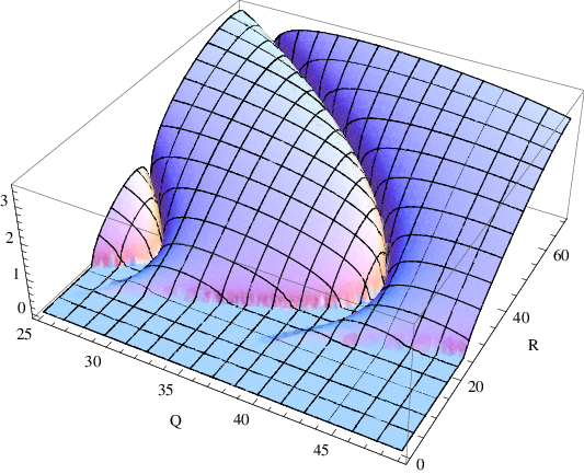
A section of the surface $\lambda_{1}(Q,R)$ for a fixed value $Q$ and a line corresponding to dissipation are presented in Fig. 4, where $Q=36$, $\mu=0.1$.

In the case under consideration the coefficient $r=r(\tau)$ changes slowly. In each $2\pi\,$-interval of the variable $s$ the multiplicator of the solution of (3.4) has the form

Consider the properties of solutions of (3.4) for the fixed value $q=36$, see Fig. 4. For $\Re\lambda-2\mu<0$ the multiplicators are less than $1$. Hence it follows that the modulus of the solution decreases on a sequence of intervals. If $\Re\lambda-2\mu>0$ then the solution growths exponentially on a sequence of intervals.

In Fig. 5 the integral index

is shown depending on time. The solution of equation (3.4) does not depend in the main on the initial data as long as $\mathit{\Lambda}<0$.

For equation (2.1) this means that when studying the general solution one can restrict oneself to the particular solution of zero initial data to the inhomogeneous equation and neglect the solution of the homogeneous equation as long as the condition $\mathit{\Lambda}<0$ is fulfilled.

The correction $y_{1}$ is determined from the differential equation

We look for a solution $y_{1}$ of the form

$\ell$ satisfying the equation

If $q$ and $r$ are in the domain where the characteristic indices of the Mathieu equation are purely imaginary and

then

for $\theta\to\infty$. The averaging over the fast variable on the right-hand side of (3.6) determines the derivative of $k$ as function of slow time . The evolution of $x_{0}$ over the fast variable is determined by the inhomogeneous equation (2.1). The dependence of $x_{0}$ upon the slow variable is explained by the slow perturbation of the coefficients of the Mathieu equation. The explicit dependence of $x_{0}$ upon the slow variable has not so far been defined. However, one can verify (3.6) by means of numerical simulation of the initial system (1.1).

The numerical solution of system (1.1) allows one to evaluate separately the left-hand side and the right-hand side of (3.6) and to determine the relative residual. We construct a numerical solution for the parameter values $\epsilon=0.2$, $\mathit{\Omega}=1$, $\omega=3$, $A=1$ and $\nu=0.1$.

The system (1.1) is solved by the Runge-Kutta method of $4\,$th order. As result we get a numerical solution $x_{\mathrm{num}}$, $y_{\mathrm{num}}$. We then divide the entire integration interval into subintervals of length $2\pi$ and on each subinterval we compute the Fourier coefficients of $\sin\theta$ and $\cos\theta$ for the function $\varepsilon y_{\mathrm{num}}$. From the data obtained in this way we evaluate the difference derivative $k^{\prime}_{\tau}$.

The averaging operator on the right-hand side of (3.6) is written in the form convenient for analytical computations. However, in numerical data the dependencies upon fast and slow variables are not separated from each other. Hence, it is not possible to directly apply formula (3.6). Instead the averaging operator over the fast variable of (3.6) is replaced by the averaging over the interval of length $O(\varepsilon^{-2})$ with centre at the point $\tau_{i}=\varepsilon^{2}t_{i}$. In this way we get the values of the right-hand side at the points $\tau_{i}$.

In Fig. 6 one compares the derivatives in $\tau$ on the left-hand side of equation (3.6), which are evaluated numerically, and the integral on the right-hand side.

We thus conclude that the substitution of the numerical solution for the genuine solution of (3.6) leads to an inessential residual.

In this section we carry out the analysis of the behaviour of the main terms of representation (3.2) under the assumption that $\lambda=\omega/\mathit{\Omega}\gg 1$. This assumption corresponds to the case of forced combinative scattering, where $\lambda$ attains the value $10^{2}$, see [3], [4].

Equation (2.1) for the main term $x_{0}$ can be obviously rewritten in the form

The asymptotics of the particular solution for large values $\lambda$ is

Our next objective is to treat equation (3.6) for $\lambda\gg 1$. To this end we substitute (4.1) into equation (3.6) and evaluate the integral explicitly. As result we get

where $\tau^{\prime}=\lambda^{-8}\tau$. This is a Hamiltonian system with Hamiltonian

The system (4) is easily seen to have a stable equilibrium point of type ‘centre’

see Fig. 7.

The amplitude of oscillations can be found from the system

In Fig. 8 the dependence of the largest $r_{+}$ (dashed curve) and smallest $r_{-}$ (solid curve) values of solutions of (4.3) upon the Hamiltonian is shown. The vertical line corresponds to $H_{0}=1/(4\pi).$

This allows one to evaluate the maximal value of the amplitude of oscillation envelope through

where

The period is determined by

where the integration is over the cycle $c$ in the complex plane of the variable $K=K_{1}+\imath K_{2}$ given by

In Fig. 9 one sees the results of numerical simulation for the solution of system (1.1) with initial data corresponding to the stationary solution

The analytical result obtained in the paper agrees well to the numerical simulation. For the values of parameters $K_{1}$ and $K_{2}$, which are used in the numerical simulation, the Hamiltonian value proves to be $H_{0}=1/(4\pi)$. In this case the amplitude of pulsations is evaluated by $\lambda^{2}\varepsilon^{-1}$. It is shown in Fig. 11. The horizontal line corresponds to $\lambda^{2}\varepsilon^{-1}$.

The explicit value for the period of envelope oscillations can be evaluated from (4.5). Our numerical simulations with parameters $A=1,\omega=3,\Omega=1,\mu=0.1,\varepsilon=0.2$ give the value $T=5264.76$ in the variable $\tau$.

In Fig. 10 the pulsations of the $y\,$-component are shown as well as the envelope superposed on them. The envelope is computed numerically as solution of system (4) with $\varepsilon=0.2$, $\lambda=3$, $A=1$. All these numerical evaluations are realized by the Adams method with the precision $10^{-10}.$

System (4) gives an approximation for determining the behaviour of functions $K_{1}$ and $K_{2}$. In Fig. 11 the solid curve corresponds to the envelope of the $y\,$-component of the solution. This curve is found from a numerical solution of system (1.1). The dashed curve $\sqrt{K_{1}^{2}+K_{2}^{2}}$ gives an approximation of the solution envelope as solution of system (4). A point $K_{1}=0,K_{2}=0$ is an unstable node equilibrium point. Initial data for system (4) correspond to the linear resonance of $y\,$-component of the solution for (1.1) in the initial stage, see Fig. 1. In Fig. 11 the vertical line shows the value of the period $T=5264.76$. It is determined numerically by expression (4.5). The horizontal line is an estimate of the maximal value $\lambda^{2}\varepsilon^{-1}$ of envelope amplitude.

It is shown in the paper that for the large time $t\sim\varepsilon^{-2}$ with $\varepsilon$ being a coupling parameter the behaviour in the main of a resonantly perturbed system of coupled oscillators is described by a Hamiltonian system. This system is studied in the physically interesting case when the quotient of oscillator frequencies $\omega/\mathit{\Omega}$ is large enough. Certain pulsations prove to occur in the solution of the initial system of coupled oscillators. The Hamiltonian system obtained allows one to evaluate the period and amplitude of these pulsations.

Acknowledgements  The research was supported by the RFBR grant 09-01-92436-KE-a, the DFG grant TA 289/4-1 and by grant 2215.2008.1 for Russian scientific schools. The first author wishes to thank the DAAD and Ministry of Education and Science of the RF for financial support in the framework of program “Mikhail Lomonosov.”

References

- [1] Bloembergen, N., The stimulated Raman effect, Amer. J. Phys. 35 (11) (1967), 989.
- [2] Fabelinskii, I. L., Seventy years of combination (Raman) scattering, Phys. Usp. 41 (1998), 1229.
- [3] Platonenko, V. T., and Khokhlov, R. V., On the mechanics of action of a combinative laser, J. of Exper. and Theor. Physics 46 (1964), no. 2, 555–559.
- [4] Akhmanov, S. A., and Nikitin, S. Yu., Physical Optics, Nauka, Moscow, 2004.
- [5] Sivukhin, D. B., General Course of Physics, 3 rd ed., Vol. IV (Optics), Fizmatlit, MFTI, Moscow, 2002, 792 pp.
- [6] Mc Goldrich, L. F., Resonant interactions among capillary-gravity waves, Journal of Fluid Mechanics 21 (1965), Issue 2, 305–331.
- [7] Ball, K., Energy transfer between external and internal gravity waves, Journal of Fluid Mechanics 19 (1964), Issue 3, 465–478.
- [8] Bogolyubov, N. N., and Mitropolskii, Yu. A., Asymptotic Methods in the Theory of Nonlinear Oscillations, Gos. Izd. Tehn.-Teor. Lit., Moscow, 1955. 449 pp.
- [9] Nayfeh, A. H., Introduction to Perturbation Techniques, John Wiley and Sons, New York, 1981.
- [10] Floquet, Gaston, Sur les equations differentielles lineaires a coefficients periodiques, Ann. Sci. École Norm. Super. 12, (1883), 47–88.
- [11] Fedoryuk, M. V., Asymptotic Methods for Linear Ordinary Differential Equations, Nauka, Moscow, 1983, 352 pp. (Russian).
- [12] Whittaker, E. T., and Watson, G. N., A Course of Modern Analysis, 4 th ed., Cambridge University Press, 1927.
- [13] Abramowitz, M., and Stegun, I. A., Handbook of Mathematical Functions, Appl. Math. Series, Nat. Bureau of Stand., Washington, 1964.