On the Support of Minimizers of
Causal Variational PrinciplesThanks: Supported in part by the Deutsche Forschungsgemeinschaft.
Abstract.
A class of causal variational principles on a compact manifold is introduced and analyzed both numerically and analytically. It is proved under general assumptions that the support of a minimizing measure is either completely timelike, or it is singular in the sense that its interior is empty. In the examples of the circle, the sphere and certain flag manifolds, the general results are supplemented by a more detailed and explicit analysis of the minimizers. On the sphere, we get a connection to packing problems and the Tammes distribution. Moreover, the minimal action is estimated from above and below.
1. Introduction
Causal variational principles were proposed in [7] as an approach for formulating relativistic quantum field theory (for surveys see [12, 16]). More recently, they were introduced in a broader mathematical context as a class of nonlinear variational principles defined on measure spaces [13]. Except for the examples and general existence results in [10, 5, 13] and the symmetry breaking effect in the discrete setting [9], almost nothing is known on the structure of the minimizers.
The present paper is the first work dedicated to a detailed analysis of the minimizing measures of causal variational principles. To introduce the problem, we begin with a brief physical motivation (Section 1.1) and then set up our mathematical framework (Section 1.2). Section 1.3 gives an overview of the obtained results. In order to make the paper easily accessible also to mathematicians who are not familiar with relativity or quantum field theory, in Section 1.1 we provide a physical introduction that is independent of the other parts of the paper and may be skipped.
1.1. Physical Background and Motivation
A relativistic quantum-mechanical particle is described by a Dirac wave function . In Minkowski space , is a four-component complex-valued wave function which depends on the spatial coordinates and time . The absolute square of a Dirac wave function has the interpretation as the probability density for the quantum mechanical particle to be at the position . Integrating this probability density over space and polarizing gives rise to a scalar product,
(where denotes complex conjugation and transposition). Note that the quantity is not a scalar, but a density. In order to obtain a Lorentz invariant scalar at a given space-time point , one must take the inner product , where is the so-called adjoint spinor. This inner product is indefinite of signature . Likewise, in the presence of a gravitational field, space-time is described by a Lorentzian manifold . In this case, the Dirac wave functions are sections of the so-called spinor bundle. Again, the spatial integral of the probability density gives rise to a scalar product . Moreover, the spinors at any space-time point are again endowed with an inner product of signature .
Let us consider a system consisting of several Dirac particles in a concrete physical configuration (say an atom or molecule). For simplicity, we here describe the system by the corresponding one-particle wave functions (for the connection to Fock spaces and the Pauli exclusion principle see for example [14]). Moreover, in order to keep the presentation as simple as possible, we assume that the number of particles is finite and that the wave functions are continuous. In order to work in a basis independent way, we consider the vector space spanned by the one-particle wave functions. Endowed with the above scalar product , this vector space is an -dimensional Hilbert space . For any space-time point , we introduce the local correlation operator as the signature operator of the inner product at expressed in terms of the Hilbert space scalar product,
Taking into account that the inner product at has signature , the local correlation operator is a symmetric operator in of rank at most four, which has at most two positive and at most two negative eigenvalues.
The local correlation operators encode how the Dirac particles are distributed in space-time and how the wave functions are correlated at the individual space-time points. We want to consider the local correlation operators as the basic objects in space-time, meaning that all geometric and analytic structures of space-time (such as the causal and metric structure, connection, curvature, gauge fields, etc.) should be deduced from the operators . The only structure besides the local correlation operators which we want to keep is the volume measure of space-time. In order to implement this concept mathematically, it is useful to identify a space-time point with the corresponding local correlation operator . Then space-time is identified with the subset . Next, we introduce the universal measure as the push-forward of the volume measure on under the mapping (thus , where is the standard volume measure). Dropping all the additional structures of space-time, we obtain a causal fermion system of spin dimension two as defined in [19, Section 1.2]:
Definition 1.1.
Given a complex Hilbert space (the “particle space”) and a parameter (the “spin dimension”), we let be the set of all self-adjoint operators on of finite rank, which (counting with multiplicities) have at most positive and at most negative eigenvalues. On we are given a positive measure (defined on a -algebra of subsets of ), the so-called universal measure. We refer to as a causal fermion system in the particle representation.
Causal fermion systems provide a general abstract mathematical framework for the formulation of relativistic physical theories. Clearly, by choosing as an infinite-dimensional Hilbert space, one can describe an infinite number of particles. The setting is so general that it allows for the description of continuum space-times (such as Minkowski space or a Lorentzian manifold), discrete space-times (such as a space-time lattice) and even so-called “quantum space-times” which have no simple classical correspondence (for examples, we refer the reader to [5, 18] and [20]). It is a remarkable fact that in causal fermion systems there are many inherent geometric and analytic structures. Namely, starting from a general causal fermion system, one can deduce space-time together with geometric structures which generalize the setting of spin geometry (see [18]). Moreover, the causal action principle gives interesting analytic structures (see [13]). In particular, one obtains a background-free formulation of quantum field theory in which ultraviolet divergences of standard quantum field theory are avoided. Since the setting also works in curved space-time, causal fermion systems are also a promising approach for quantum gravity. We refer the interested reader to the review article [18] as well as to the preprints [11, 17, 6].
We now outline how to deduce the geometric and analytic structures which will be relevant in this paper. Starting from a causal fermion system , one defines space-time as the support of the universal measure, . On , we consider the topology induced by . The causal structure is encoded in the spectrum of the operator products :
Definition 1.2.
For any , the product is an operator of rank at most . We denote its non-trivial eigenvalues by (where we count with algebraic multiplicities). The points and are called timelike separated if the are all real. They are said to be spacelike separated if all the are complex and have the same absolute value. In all other cases, the points and are said to be lightlike separated.
The main analytic tool is the causal variational principle defined as follows. For two points we define the spectral weight of the operator products and by
We also introduce the
| (1.1) |
For a given universal measure on , we define the non-negative functionals
| (1.2) | ||||
| (1.3) |
The causal action principle is to
| minimize for fixed |
under variations of the universal measure. These variations should keep the total volume unchanged, which means that a variation should satisfy the conditions
for all (where denotes the total variation of a measure; see [21, §28]). Depending on the application, one may impose one of the following constraints:
- (C1)
The trace constraint:
- (C2)
The identity constraint:
- (C3)
Prescribing eigenvalues: We denote the non-trivial eigenvalues of counted with multiplicities by and order them such that
For given constants , we impose that
(1.4)
Moreover, one may prescribe properties of the universal measure by choosing a measure space and restricting attention to universal measures which can be represented as the push-forward of ,
| (1.5) |
One then minimizes the action under variations of the mapping .
The Lagrangian (1.1) is compatible with our notion of causality in the following sense. Suppose that two points are spacelike separated (see Definition 1.2). Then the eigenvalues all have the same absolute value, so that the Lagrangian (1.1) vanishes. Thus pairs of points with spacelike separation do not enter the action. This can be seen in analogy to the usual notion of causality where points with spacelike separation cannot influence each other.
In the present paper, we restrict attention to a special class of causal variational principles, as we now explain. First, we always assume that the number of particles is finite. Then is finite-dimensional, and is a locally compact topological space. Moreover, we always have the situation in mind when the above constraint (C3) is present. In this case, we may replace by the set of those operators which satisfy the constraints (1.4). Then becomes a compact topological space. In this so-called compact setting, the causal variational principle is mathematically well-defined, even without imposing the constraint (1.3). For simplicity, we shall disregard this constraint. Next, we do not want to use (1.5) to prescribe any properties of . Instead, we allow to be any normalized positive Borel measure on . This is what we mean by the continuous setting. Finally, we assume that the Lagrangian (1.1) is of the form
| (1.6) |
This assumption is automatically satisfied in the case of spin dimension one. Namely, in this case the eigenvalues and are either both real, or else they form a complex conjugate pair. In the first case, the Lagrangian is positive and smooth, whereas in the second case it vanishes identically. Hence can indeed be written in the desired form (1.6).
The above specializations are made in order to make the mathematical problem manageable. Despite the major simplifications, our results shed some light on the general structure of minimizers of causal variational principles. Qualitatively speaking, our results reveal a mechanism which favors discrete over continuous configurations. This mechanism seems to have interesting physical implications: First, thinking of a quantum space-time, the discreteness of the minimizing measure means that the causal action principle should arrange that space-time is discrete on the Planck scale. This effect would be very desirable because it would resolve the ultraviolet problems of quantum field theory. Another implication is related to field quantization. To explain the connection, let us consider a family of universal measures which describes a physical system where a classical amplitude is varied continuously. Then our “discreteness results” mean that some discrete values of should be favored. As a consequence, the amplitude no longer takes continuous values, but it should be “quantized” to take the discrete values for which the causal action has a local minimum. Finally, our “discreteness results” might also account for effects related to the wave-particle duality and the collapse of the wave function in the measurement process. For a more detailed physical discussion we refer to [8, 15].
1.2. The Mathematical Setup
We now introduce our mathematical setting. Let be a smooth compact manifold (of arbitrary dimension). For a given function
| (1.7) | ||||
| and strictly positive on the diagonal: | (1.8) |
we define the Lagrangian by
| (1.9) |
Introducing the action by
| (1.10) |
our action principle is to
| minimize under variations of | (1.11) |
where denotes the set of all normalized positive regular Borel measures on . In view of the symmetric form of (1.10), it is no loss of generality to assume that is symmetric in and . Therefore, it is natural to assume that also is symmetric (1.7). If (1.8) were violated, every measure supported in the set would be a minimizer. Thus the condition (1.8) rules out trivial cases.
The existence of minimizers follows immediately from abstract compactness arguments (see [13, Section 1.2]).
Theorem 1.3.
The infimum of the variational principle (1.11) is attained in .
Note that the minimizers will in general not be unique. Moreover, the abstract framework gives no information on what the minimizers look like.
The notion of causality can now be introduced via the sign of .
Definition 1.4 (causal structure).
We define the sets
| open lightcone | |||||
| closed lightcone | |||||
Thus if and only if the function changes sign in every neighborhood of .
Our action is compatible with the causal structure in the sense that if and have lightlike or spacelike separation, then the Lagrangian vanishes, so that the pair does not contribute to the action. Note that for a given minimizer , we have similarly a causal structure on its support.
In order to work in more specific examples, we shall consider the following three model problems.
- (a)
Variational principles on the sphere:
We consider the setting of [13, Chapter 1] in the case (see also [13, Examples 1.5, 1.6 and 2.8]). Thus for a given parameter , we let be the space of Hermitian -matrices whose eigenvalues are equal to and . Writing a matrix as a linear combination of Pauli matrices,we can describe by the unit vector (here denotes the scalar product in ). Thus can be identified with the unit sphere . The function is computed in [13, Example 2.8] to be
(1.12) This function depends only on the angle between the points defined by , which clearly coincides with the geodesic distance of and .
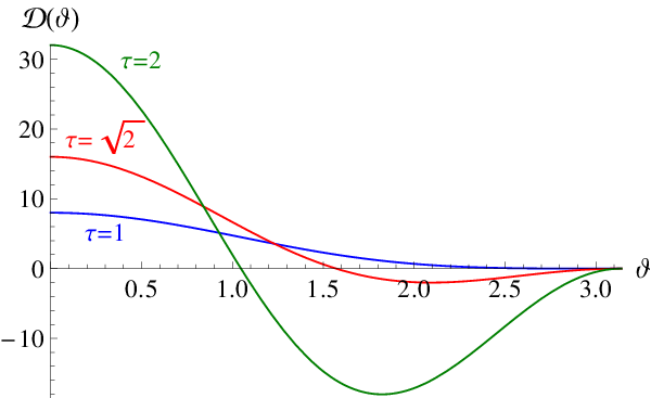
Figure 1. The function . Considered as function of , has its maximum at and is minimal if . Moreover, . Typical plots are shown in Figure 1. In the case , the function has two zeros at and
(1.13) In view of (1.9), the Lagrangian is positive if and only if . Thus is an open spherical cap, and is its closure together with the antipodal point of ,
If is increased, the opening angle of the lightcones gets smaller. In the degenerate case , the function is decreasing, non-negative and has exactly one zero at . Hence the Lagrangian coincides with . All points on the sphere are timelike separated except for the antipodal points. The lightcones are given by and .
- (b)
Variational principles on the circle:
In order to simplify the previous example, we set . For we again choose (1.12). - (c)
Variational principles on the flag manifold :
As in [13, Chapter 1], for a given parameter and an integer parameter , we let be the space of Hermitian -matrices of rank two, whose nontrivial eigenvalues are equal to and . Every is uniquely described by the corresponding eigenspaces and . By considering the chain , can be identified with an element of the flag manifold , the space of one-dimensional subspaces contained in a two-dimensional subspace of (see [22]). It is a -dimensional compact manifold. Every gives rise to the mapping on . This resulting group action of on acts transitively, making a homogeneous space (see [22] for details).For two points , we denote the two non-trivial eigenvalues of the matrix product by and define the Lagrangian by
This Lagrangian is -invariant. In order to bring it into a more convenient form, we first note that by restriction to the image of , the characteristic polynomial of changes only by irrelevant factors of ,
where denotes the orthogonal projection to . It follows that and are the eigenvalues of the -matrix . In particular,
because the operator again has at most one positive and one negative eigenvalue. Moreover, the relation shows that the two eigenvalues are either both real and have the same sign or else they form a complex conjugate pair, in which case the Lagrangian vanishes. Finally, using that , the Lagrangian can be written in the form (1.9) with
(1.14)
We finally comment on the limitations of our setting and mention possible generalizations. First, we point out that our structural results do not immediately apply in the cases when is non-compact or when additional constraints are considered (see [13, Chapter 2]). However, it seems that in the non-compact case, our methods and results could be adapted to the so-called moment measures as introduced in [13, Section 2.3]. A promising strategy for handling additional constraints would be to first derive the corresponding Euler-Lagrange equations, treating the constraints with Lagrange multipliers (for details see [1]). Then one could try to recover these Euler-Lagrange equations as those corresponding to an unconstrained variational problem on a submanifold , where our methods could again be used. We finally point out that in the case of higher spin dimension , it is in general impossible to write the Lagrangian in the form (1.9) with a smooth function , because the Lagrangian is in general only Lipschitz continuous in the open light cone. A possible strategy would be to first show that the support of lies on a submanifold , and then to verify that by restricting to , it becomes smooth in the open lightcones.
1.3. Overview of the Main Results
We now outline our main results. In Section 2, we present numerical results on the sphere (see Figure 3) and discuss all the main effects which will be treated analytically later on. In Section 3, we derive general results on the structure of the minimizers. We first derive the corresponding Euler-Lagrange equations and conditions for minimality (see Lemma 3.4 and Lemma 3.5). We then prove under general assumptions that the minimizers are either generically timelike (see Definition 3.8) or else the support of the minimizing measure defined by
is singular in the sense that its interior is empty (see Theorems 3.16 and 3.18). In the following sections, we apply these general results to our model examples and derive more detailed information on the minimizers. In Section 4, we consider the variational principle on the circle. After briefly discussing numerical results (see Figure 4), we prove a “phase transition” between generically timelike minimizers and minimizers with singular support and construct many minimizers in closed form (see Corollary 4.2 and Theorem 4.4). In Section 5, the variational principle on the sphere is considered. We again prove the above phase transition (see Corollary 5.1) and estimate the action from above and below (see Figure 6 and Proposition 5.3). Finally, in Section 6 we apply our general results to flag manifolds (see Theorem 6.1). Moreover, we prove that minimizers with singular support exist (see Theorem 6.2) and give an outlook on generically timelike minimizers.
We close the introduction with a remark on our methods. Generally speaking, our proofs are based on a detailed functional analytic study of first and second variations. The analysis of second variations reveals that, for a minimizing measure , a certain operator on a Hilbert space is positive (see Lemma 3.5). This positivity property is the key for analyzing the support of . Our method is to proceed indirectly and to show that if the support does not have the desired properties, then there is a vector with , a contradiction. Clearly, the difficulty is to construct the vector ; here we use the specific form of our variational principle.
The method of relating properties of the minimizer to positivity properties of a corresponding operator bears some similarity to the methods in [26, 3]. Namely, in [26] it is shown that if a certain pair potential is positive in momentum space, then there are discrete ground states. In [3], on the other hand, it is shown for a repulsive pair potential that in a suitable limit where the number of particles tends to infinity, the particles are distributed uniformly on a -sphere. The methods in both of these papers cannot be compared directly, because the mathematical structure of the considered variational problems is quite different from our causal variational principles. In particular, our variational principles are not formulated for particle configurations, but for general measures. Moreover, we make essential use of the fact that our pair potential is not smooth, but only Lipschitz continuous.
2. Numerical Results on the Sphere
In order to motivate our general structural results, we now describe our findings in a numerical analysis of the variational principle on the sphere (see Example (a) on page (a)). Clearly, in a numerical study one must work with discrete configurations. Our first attempt is to choose a finite number of points and to let be the corresponding normalized counting measure, i.e.
| (2.1) |
Then the action (1.10) becomes
| (2.2) |
By varying the points for fixed , we obtain a minimizer . Since every normalized positive regular Borel measure can be approximated by such counting measures, we can expect that if we choose sufficiently large, the measure should be a good approximation of a minimizing measure (more precisely, we even know that as with convergence in the weak -topology).
If is sufficiently large, the opening angle of the lightcones is so small that the points can be distributed on the sphere such that any two different points are spacelike separated. In this case, the action becomes
| (2.3) |
and in view of (2.2) this is indeed minimal. The question for which such a configuration exists leads us to the Tammes problem, a packing problem where the points are distributed on the sphere such that the minimal distance between distinct points is maximized, see [25]. More precisely, we know that the Tammes distribution is a minimizer of our action if is so large that . Until now, the Tammes problem is solved only if and for (for details see [4] and the references therein). For special values of , the solutions of the Tammes problem are symmetric solids such as the tetrahedron (), the octahedron (), the icosahedron () and the snub cube (). Moreover, much research has been done on the numerical evaluation of spherical codes, mostly by N.J.A. Sloane, with the collaboration of R.H. Hardin, W.D. Smith and others, [25], obtaining numerical solutions of the Tammes problem for up to points.
In the case , the measure was constructed numerically using a simulated annealing algorithm11 1 We use the “general simulated annealing algorithm” by J. Vandekerckhove, © 2006, http://www.mathworks.de/matlabcentral/fileexchange/10548.. In order to get optimal results, we used this algorithm iteratively, using either a Tammes distribution or previous numerical distributions as starting values. Using that depends smoothly on , it is useful to increase or decrease in small steps, and to use the numerical minimizer as the starting configuration of the next step. In Figure 2, the numerically found is plotted for different values of as a function of the parameter .

The resulting plots look rather complicated. The considered values for are too small for extrapolating the limiting behavior as . Nevertheless, one observation turned out to be very helpful: Near , the plots for different values of look the same. The reason is that some of the coincide, forming “clusters” of several points. For example, in the case , the support of consists of only six distinct points, each occupied by two . A similar “clustering effect” also occurs for higher if is sufficiently large.
These findings give the hope that for large , the minimizers might be well-approximated by a measure supported at a few cluster points, with weights counting the number of points at each cluster. This was our motivation for considering a weighted counting measure. Thus for any fixed , we choose points and corresponding weights with
We introduce the corresponding measure in generalization of (2.1) by
| (2.4) |
Seeking for numerical minimizers by varying both the points and the weights , we obtain the plots shown in Figure 3.

These plots suggest the following structure of the minimizers. Let us denote the minimizing weighted counting measure for given by . Then for any fixed , the series is monotone decreasing (this is obvious because every can be realized by a weighted counting measure with summands by choosing weights equal to zero). The important observation is that there is an integer from which point on the series stays constant, i.e.
This implies that the measure is also a minimizer in the class of all Borel measures. This leads us to the following
Conjecture 2.1.
For any , there is a minimizer of the variational problem on the sphere which is a weighted counting measure supported at points.
From Figure 3 we can read off the value of as a function of . More precisely, if , then is not minimal and coincides with the action for the Tammes distribution (2.3). The corresponding curves are labelled in Figure 3 by . If , on the other hand, is minimal and lies on the thick curve in Figure 3. Obviously, increases as gets larger. This corresponds to the fact that for increasing , the opening angle of the light cones gets smaller, so that it becomes possible to distribute more points on the sphere which are all spatially separated from all the other points.
The more detailed numerical study of the minimizers showed another interesting effect. For values , we found many different minimizers of different form. They all have the property that they are completely timelike in the sense that all points in the support of the minimizing measure have timelike or lightlike separation from all the other points. We found minimizers supported on an arbitrarily large number of points. If, on the other hand , all minimizers were supported on at most points, indicating that every minimizing measure should be discrete with finite support. The intermediate value corresponds to the opening angle of the light cones.
Conjecture 2.2.
If , every minimizer is completely timelike. If, conversely, , every minimizing measure is discrete with finite support.
More graphically, one can say that for , our variational principle spontaneously generates a discrete structure on the sphere. The two regions and can also be understood as two different phases of the system, so that at we have a phase transition from the completely timelike phase to the discrete phase.
The above numerical results will serve as the guideline for our analysis. More precisely, the completely timelike phase will be analyzed in Section 3.2 using the notion of “generically timelike”, whereas in Section 3.3 we will develop under which assumptions and in which sense the support of the minimizing measure is discrete or “singular”. The phase transition is made precise in Theorem 3.16 and 3.18 by stating that minimizing measures are either generically timelike or singular.
3. General Structural Results
We now return to the general variational principle (1.11) with the Lagrangian of the form (1.9) and (1.7) on a general smooth compact manifold . Let us introduce some notation. For a given measure , we define the functions
| (3.1) | ||||
| (3.2) |
Moreover, we denote the Hilbert space by and introduce the operators
(we use the consistent notation that a subscript always denotes the corresponding operator on ).
Lemma 3.1.
The operators and are self-adjoint and Hilbert-Schmidt. The eigenfunctions of (and ) corresponding to the non-zero eigenvalues can be extended to Lipschitz-continuous (respectively smooth) functions on .
Proof.
We only consider , as the proof for is analogous. The self-adjointness follows immediately from the fact that is symmetric. Moreover, as the kernel is smooth and is compact, we know that
This implies that is Hilbert-Schmidt (see [23, Theorem 2 in Section 16.1]).
Suppose that with . Then the representation
shows that (recall that is smooth according to (1.7)). ∎
The following notions characterize properties of and the function that will be needed later on.
Definition 3.2.
A measure is a homogenizer of if and both functions
are constant on . The function is called homogenizable if a homogenizer exists.
In Examples (a) and (b) in Section 1.2, we can always choose the standard normalized volume measure as the homogenizer. More generally, in Example (c) we choose for the normalized Haar measure, obtained by introducing a -invariant metric on and taking the corresponding volume form (see for example [2, Section I.5]).
The next proposition gives a sufficient condition for a homogenizer to be a minimizer.
Proposition 3.3.
If , the homogenizer is a minimizer of the variational principle (1.11).
Proof.
We denote the constant function on by . If is a homogenizer, this function is an eigenfunction of , which can be completed to an orthonormal eigenvector basis of with and corresponding eigenvalues .
Using an approximation argument in the -topology, it suffices to show that
for any with and . We write in the eigenvector basis ,
The condition implies that . Thus
∎
3.1. The Euler-Lagrange Equations
Let us assume that is a minimizer of the variational principle (1.11),
We now derive consequences of minimality. In the first lemma, we consider first variations of to obtain the Euler-Lagrange equations corresponding to our variational principle. The second lemma, on the other hand, accounts for a nonlinear effect.
Lemma 3.4.
(The Euler-Lagrange equations)
| (3.3) |
Proof.
Since is continuous and is compact, there clearly is with
| (3.5) |
We consider for the family of measures
where denotes the Dirac measure supported at . Substituting this formula in (1.10) and differentiating, we obtain for the first variation the formula
Since is a minimizer, is positive. Combining this result with (3.4) and (3.5), we obtain the relations
It follows that is constant on the support of , giving the result. ∎
The statement of Lemma 3.4 implies that for any ,
| (3.6) |
showing that the constant function is an eigenvector of the operator corresponding to the eigenvalue . However, the statement (3.3) is stronger because it gives information on even away from the support of .
Lemma 3.5.
The operator is positive (but not necessarily strictly positive).
Proof.
Assume that the lemma is wrong. Then, as is a compact and self-adjoint operator (see Lemma 3.1), there exists an eigenvector corresponding to a negative eigenvalue, with . We consider the family of measures
In view of Lemma 3.1, is continuous and therefore bounded. Thus for sufficiently small , the measure is positive. In view of (3.6), the functions and are eigenfunctions corresponding to different eigenvalues. Hence these eigenfunctions are orthogonal. Thus
showing that is again normalized. Finally, again using the orthogonality,
Thus is an admissible variation which decreases the action, a contradiction. ∎
This lemma has useful consequences. We first derive a positivity property of the Lagrangian when evaluated on a finite number of points in the support of .
Corollary 3.6.
For a finite family (with ), the Gram matrix defined by
is symmetric and positive semi-definite.
Proof.
Given and a vector , we set
where is a ball of radius (in any given coordinate system). Lemma 3.5 implies that . Taking the limit , it follows that
∎
We next derive a simple criterion which guarantees that a minimizing measure cannot be supported on the whole manifold .
Corollary 3.7.
Assume that there is a bounded regular Borel measure (not necessarily positive) such that
Then the support of a minimizing measure cannot contain the support of ,
Proof.
If we assume, conversely, that , the measure can be approximated by measures of the form with (in the sense that in the weak--topology). As a consequence, the expectation value is negative for large , in contradiction to Lemma 3.5. ∎
This corollary explains why minimizers have the tendency of being supported on proper subsets of . But the argument is too weak for concluding discreteness. In order to get more detailed information on the form of the minimizing measures, we need more advanced notions and methods, which we now introduce.
3.2. Generically Timelike Minimizers
Definition 3.8.
A minimizing measure is called generically timelike if the following conditions hold:
- (i)
for all .
- (ii)
The function defined by (3.2) is constant on .
This constant can easily be computed:
Lemma 3.9.
Suppose that is a generically timelike minimizer. Then
Proof.
In view of property (i), and coincide on the support of . Thus
Carrying out one integral using (3.2), we obtain
Using property (ii) gives the result. ∎
In the remainder of this subsection, we assume that is homogenizable (see Definition 3.2) and denote the homogenizer by .
Lemma 3.10.
If has only a finite number of negative eigenvalues, then the kernel has the representation
| (3.7) |
with , , , and , where in the case the series converges uniformly.
Proof.
By definition of the homogenizer, the function is an eigenfunction of the operator . Denoting the corresponding eigenvalue by , we obtain the spectral representation (3.7).
If is positive, the uniform convergence is an immediate generalization of Mercer’s theorem (see [23, Theorem 11 in Chapter 30], where we replace the interval by the compact space , and the Lebesgue measure by the measure ). In the case when has a finite number of negative eigenvalues, we apply Mercer’s theorem similarly to the operator with kernel , where are the negative eigenvalues with corresponding eigenfunctions . By construction, this operator is positive, and in view of Lemma 3.1 its kernel is continuous. ∎
Lemma 3.11.
Suppose that is a generically timelike minimizer and that the operator has only a finite number of negative eigenvalues. Then
Proof.
Proposition 3.12.
Suppose that is a positive operator on the Hilbert space . Then
In the case of equality, every minimizer is generically timelike.
Proof.
If is positive, all the parameters in (3.7) are positive. It follows that for every measure ,
| (3.9) |
Let us assume that equality holds. It then follows from (3.9) that and coincide on the support of and thus for all . Moreover, we find from (3.7) or (3.8) that
and thus
It follows that is a constant. We conclude that is generically timelike. ∎
This proposition can be used to construct generically timelike minimizers.
Corollary 3.13.
Suppose that is a positive operator on . Assume that the function has the following properties:
- (a)
for all .
- (b)
Then the measure is a generically timelike minimizer.
Proof.
We conclude this section by stating obstructions for the existence of generically timelike minimizers.
Proposition 3.14.
Assume that one of the following conditions holds:
- (I)
The operator has only a finite number of negative eigenvalues, and the eigenvalue in the decomposition (3.7) is non-positive.
- (II)
For every there is a point with (“condition of disjoint lightcones”).
- (III)
For every there is a point with and (“condition of antipodal points”).
Then there are no generically timelike minimizers.
Proof.
We first show that . Namely, choosing in the support of a minimizing measure , we know from (1.8) and the continuity of that there is a neighborhood of and such that for all . It follows that
Case (I) is obvious in view of Lemma 3.11 and the fact that . To prove the remaining cases (II) and (III), we assume conversely that there exists a generically timelike minimizer . Choosing a point , we know from property (i) in Definition 3.8 that . In case (II), we choose with to obtain
in contradiction to Lemma 3.9.
In case (III), we know that . If , the estimate
again gives a contradiction, where in (*) we used that . If conversely , then (where we again used that ). Hence the integral in (3.2) reduces to a sum over two points,
| (3.10) |
In view of our assumption (1.8), we know that and . On the other hand, the relation shows that . Hence there is a point . It follows that (because ) and also (because and thus ). Using these inequalities in (3.10), we again find that , a contradiction. ∎
It is interesting to ask what the support of a generically timelike minimizer may look like. The next proposition (which will not be used later on) quantifies that must be “sufficiently spread out.”
Proposition 3.15.
Assume that is a generically timelike minimizer and that the operator has only a finite number of negative eigenvalues. Then every real function with
| (3.11) |
changes its sign on the support of (here is again the homogenizer of Definition 3.2).
Proof.
We return to the spectral decomposition (3.7) of the operator . Since the eigenfunctions are orthogonal in , we know that
Representing in an eigenvector basis of and using (3.11), we find
with complex coefficients . Integrating with respect to , we can apply Lemma 3.11 to obtain
Hence changes its sign on the support of . ∎
3.3. Minimizers with Singular Support
We now state results on the support of a minimizing measure.
Theorem 3.16.
Let be a smooth compact manifold. Assume that is symmetric (1.7) and equal to one on the diagonal, . Furthermore, we assume that for every and , there is a smooth curve joining the points and , along which has a non-zero derivative at , i.e.
| (3.12) |
where we parametrized the curve such that . Then the following statements are true:
- (A)
If , are real analytic, then a minimizing measure is either generically timelike or .
- (B)
If is smooth and if there is a differential operator (of any finite order) on which vanishes on the constant functions such that
(3.13) then .
A typical example for is the Laplacian corresponding to a Riemannian metric on . Note that the condition (3.12) implies that for every , the set is a smooth hypersurface, which the curve intersects transversely (in the applications of Section 4 and 5, this set will coincide with , but this does not need to be true in general).
The condition (3.12) can be removed if, instead, we make the following symmetry assumption.
Definition 3.17.
The function is called locally translation symmetric at with respect to a curve with if there is and a function such that the curve is defined on the interval and
Theorem 3.18.
Let be a smooth compact manifold. Assume that is symmetric (1.7) and strictly positive on the diagonal (1.8). Furthermore, we assume that for every and , there is a smooth curve joining the points and such that is locally translation symmetric at with respect to , and such that the function changes sign at (where we again parametrize the curve such that ). Then statement (A) of Theorem 3.16 holds, provided that the curve is analytic in a neighborhood of . Assume, furthermore, that there is with
| (3.14) |
Then statement (B) of Theorem 3.16 again holds.
In the smooth setting, the above theorems involve quite strong additional assumptions (see (3.12), (3.13) and (3.14)). The following counter example shows that some conditions of this type are necessary for the statements of these theorems to be true22 2 We would like to thank Robert Seiringer for pointing out a similar example to us..
Example 3.19.
Let be non-negative even functions with
We introduce the function by
| (3.15) |
where is the standard volume measure, and denotes the geodesic distance (taking values in ). Note that the two summands in (3.15) have disjoint supports, and thus the corresponding Lagrangian (1.9) is simply
We again consider and as the integral kernels of corresponding operators and on the Hilbert space .
First, it is obvious that is symmetric and constant on the diagonal. Next, it is clear by symmetry that the measure is a homogenizer (see Definition 3.2). Moreover, writing as , where is the operator with integral kernel , one sees that the operator is positive. Thus by Proposition 3.3, the measure is minimizing. If the function is non-trivial, there are points which are spacelike separated, so that this minimizer is not generically timelike. Also, its support obviously has an empty interior. We have thus found a minimizing measure which violates statement (A) of Theorem 3.16.
The remainder of this section is devoted to the proof of the above theorems. We begin with a simple but very useful consideration. Suppose that for given , the boundary of the light cone does not intersect the support of . As the support of is compact, there is neighborhood of such that
Thus introducing the measure , the function can for all be represented by
| (3.16) |
In the following two lemmas, we make use of this identity in the smooth and analytic settings.
Lemma 3.20.
If (3.13) holds, then for every the set is nonempty.
Proof.
Lemma 3.21.
Suppose that and are real analytic. Assume that there exists a point such that . Then is generically timelike and .
Proof.
We introduce on the function
Then is real analytic and, according to (3.16), it coincides on with the function . Since , the Euler-Lagrange equations in Lemma (3.4) yield that in a neighborhood of . Hence in a neighborhood of , and the real analyticity implies that
It follows that
| (3.17) |
and thus . Since and is normalized, we conclude that . Thus . Moreover, the inequality in (3.17) becomes an equality, showing that on the support of . Thus is indeed generically timelike. ∎
To complete the proof of Theorems 3.16 and 3.18, it remains to show the following statement:
| (3.18) |
We proceed indirectly and assume that there is a point . Our strategy is to choose points in a neighborhood of such that restricted to the set is not positive semi-definite, in contradiction to Corollary 3.6. The points will all lie on a fixed smooth curve which joins and chosen as in the statement of the theorems. We parametrize such that and , and by extending the curve we can arrange that the curve is defined on the interval for suitable . By the assumptions in Theorems 3.16 and 3.18, we know that changes sign at . Depending on the sign of , we introduce the “chain” of points
| (3.19) |
(thus has timelike separation from , lightlike separation from , and spacelike separation from ). Then by construction, , whereas all the other points of the chain are spacelike or lightlike separated from .
For the proof of Theorem 3.16, it suffices to consider a chain of three points.
Lemma 3.22.
Proof.
We set for . Using that is symmetric and that , we know that
Thus the linear term in a Taylor expansion vanishes,
where we set
As the function is smooth, we can again expand it in a Taylor series,
We thus obtain
Setting and using that , the result follows. ∎
Proof.
Assume, conversely, that for there is a point . We choose the chain as in Lemma 3.22. We use the notation of Corollary 3.6 in case , setting . Choosing the vector as , we can apply Lemma 3.22 to obtain
Furthermore, using (3.12), we know that
with . Thus, choosing with , it is
For sufficiently small , the matrix in this equation has a negative determinant, in contradiction to Corollary 3.6. ∎
This completes the proof of Theorem 3.16.
In order to finish the proof of Theorem 3.18, we first remark that, combining the symmetry of with the assumption that is locally translation symmetric at with respect to , we know that . After rescaling, we can assume that . A Taylor expansion of then yields the following simplification and generalization of Lemma 3.22,
| (3.21) |
where the real coefficients only depend on and the curve .
Proof.
Let us first verify that in the real analytic case, there is a such that (3.14) holds. Namely, assuming the contrary, all the -derivatives of the function vanish. As the function is real analytic in a neighborhood of (as the composition of analytic functions is analytic), it follows that this function is locally constant. This contradicts the fact that changes sign at .
Assume conversely that for there is a point . We choose the chain as in (3.19) with . We use the notation of Corollary 3.6 in case . Then the Gram matrix becomes
Using the expansion (3.21) for , we obtain
| (3.22) |
where denotes the matrix where all the matrix entries (also the off-diagonal entries) are equal to one, and is the matrix whose element has the value .
Let us construct a vector such that the expectation value is of the order . To this end, we take for a non-trivial solution of the linear equations
| (3.23) |
Then and for all ,
Each summand involves a power of and a power of , where always one of these powers is smaller than . Thus all summands vanish according to (3.23),
We conclude that in the expectation value with according to (3.22) all the terms except for the error term vanish,
Moreover, the solution can always be normalized by , because setting to zero, the system of equations (3.23) can be rewritten with the square Vandermonde matrix, which has a trivial kernel.
We next consider the setting of Corollary 3.6, but now with and . Using (3.14) together with the fact that the points and are timelike separated, we find that
| (3.24) |
for . We choose the vector as with (and as above). Then
where we combined (3.24) with our normalization , and used that is not timelike separated from . For sufficiently small , the matrix in this equation has a negative determinant, in contradiction to Corollary 3.6. ∎
This completes the proof of Theorem 3.18.
4. The Variational Principles on the Circle
As a simple starting point for a more detailed analysis, we now consider the variational principles on the circle (see Example (b) on page (b)). We first discuss numerical results, which again show the “critical behavior” discussed in Section 2 for the variational principle on . Applying the previous structural results, we will prove this critical behavior and show, under generic assumptions, that the minimizing measure is supported at a finite number of points. Moreover, we will give many minimizers in closed form.
Our numerical methods and results are similar to those on , as we now describe. We again consider the weighted counting measure (2.4). As the starting configuration we choose, in analogy of the Tammes distribution on a uniform distribution of points on the circle,
| (4.1) |
with uniform weights . Minimizing as in Section 2 with a simulated annealing algorithm, we obtain the results shown in Figure 4.

The numerical findings indicate that the minimizing measure is supported at a finite number of points . This number can be stated explicitly by
| (4.2) |
where , as given by (1.13), denotes the opening angle of the lightcone. The number increases with , with discontinuous “jumps” at the values
| (4.3) |
Besides the discrete nature of the minimizers, the numerical results reveal that at (corresponding to ), the structure of the minimizers changes completely. Just as in Section 2, this effect can be understood as a phase transition. More precisely, if , every minimizer is generically timelike. If we further decrease (i.e., for every fixed ), we even found a large number of minimizing measures, supported at different numbers of points with strikingly different positions. However, if , the minimizer is unique (up to rotations on ), is supported at points, and is not generically timelike.
In the remainder of this section, we make this picture rigorous. First, the operator can be diagonalized explicitly by plane waves (where , and is the angle). This gives rise to the decomposition
where
| (4.4) |
and similarly and . In the case , all eigenvalues , and are non-negative, and we can apply Proposition 3.12 to obtain
For sufficiently small , the uniform distribution of points on the circle (4.1) gives a family of generically timelike minimizers:
Lemma 4.1.
If and is so small that for all , then is a generically timelike minimizer. Every other minimizer is also generically timelike.
Proof.
A straightforward calculation using the identities
yields for any ,
In particular, one sees that .
Applying this lemma in the case gives the following result.
Corollary 4.2.
If , every minimizer is generically timelike.
More general classes of generically timelike minimizers can be constructed explicitly with the help of Corollary 3.13. In particular, one can find minimizing measures which are not discrete. For the details we refer to the analogous measure on given in Example 5.2.
Having explored the case , we proceed with the case . As already stated, the closed lightcones are given by
Therefore, if (or equivalently ), the condition of antipodal points (see Proposition 3.14) is satisfied. Thus there are no generically timelike minimizers. As the condition (3.12) is obvious, we can apply Theorem 3.16 (A) and conclude that
| (4.5) |
Using results and methods from Section 3.3, we we will be able to explicitly construct all minimizers under the additional technical assumption that
We first introduce a descriptive notation:
Definition 4.3.
A chain of length is a sequence of pairwise distinct points such that for all .
Theorem 4.4.
If , then the support of every minimizer is a chain (with as given by (4.2)). The minimal action is
| (4.6) |
where . The minimizing measure is unique up to rotations on .
An example for the support of the minimizing measure is shown in Figure 5.

Up to rotations, the points of the chain can be written as
| (4.7) |
In the special cases , the minimizer is the measure with equal weights supported on the uniform distribution . In the general case, the weights will not all be the same, as will be specified below.
For the proof of Theorem 4.4 we proceed in several steps.
Lemma 4.5.
If , the minimal action is attained for a measure supported on a chain . In the case , every minimizing measure is a chain.
Proof.
Let be a minimizing measure. We first note that every chain in the support of must have finite length, because otherwise would have to be irrational. As a consequence, would be a dense set of , in contradiction to the discreteness of (see (4.5)). Let us assume that the support of is not a chain.
We let be a chain, which is maximal in the sense that it cannot be extended. Set . We consider variations of where we rotate by a small angle , leaving the weights on as well as unchanged. The fact that cannot be extended implies that that these variations are smooth in at . The minimality of implies that
| (4.8) |
On the other hand, differentiating (1.12), one finds that the function restricted to is concave,
Comparing with (4.8), we conclude that vanishes for all and . In the case that , this implies that , a contradiction. In the remaining case , we can subdivide the circle into two disjoint arcs and such that and . The opening angle of can be chosen larger than times the length of , giving an a priori upper bound on the length of .
By further rotating , we can arrange that the chain can be extended by a point in , without changing the action. If the extended chain equals the support of , the proof is finished. Otherwise, we repeat the above argument with replaced by its extension. In view of our a priori bound on the length of , this process ends after a finite number of steps. ∎
Lemma 4.6.
Suppose that is a minimizing measure supported on a chain. If , the length of this chain is at most .
Proof.
From the last two lemmas we conclude that every minimizer is supported on one chain of length at most . If we parametrize the points as in (4.7), the only contributions to the action come from and . Using Lagrange multipliers, the optimal weights are calculated to be
where we set
The corresponding action is computed to be , giving the formula in (4.6). Using this explicit value of the action, we obtain the following result.
Lemma 4.7.
Suppose that is a minimizing measure supported on a chain. Then the length of this chain is at least .
Proof.
For a chain of length , the only contributions to the action come from , . The corresponding optimal weights are computed by . The resulting action is
This is easily verified to be strictly larger than the value of the action in (4.6). ∎
This completes the proof of Theorem 4.4.
We finally remark that if lies in the interval where Theorem 4.4 does not apply, the numerics show that the minimizing is again the measure supported on the chain of length , with one exception: If is in the interval with , a chain of length gives a lower action than the chain of length . In this case, the Gram matrix (4.10) is indeed positive definite, so that the argument in Lemma 4.7 fails.
5. The Variational Principles on the Sphere
We now come to the analysis of the variational principles on the sphere (see Example (a) on page 4). Applying Theorem 3.16 (A) with the curve chosen as the grand circle joining and , we immediately obtain that every minimizing measure on is either generically timelike or else . The numerics in Section 2 indicated that these two cases are separated by a “phase transition” at . We will now prove that this phase transition really occurs. Moreover, we will develop methods for estimating the minimal action from above and below. Many of these methods apply just as well to the general setting introduced in Section 1.2 (see (1.7)–(1.11)).
5.1. Generically Timelike Minimizers
We first decompose in spherical harmonics. A short calculation yields in analogy to (3.7) the decomposition
where the eigenvalues are given by
| (5.1) |
In particular, the operator is positive if .
If , there is a large family of minimizers, as we now discuss. The simplest example is the octahedron: Denoting the unit vectors in by , we consider the measure supported at with equal weights . Obviously, the condition (i) in Definition 3.8 is satisfied. Moreover, for any one calculates
Thus Proposition 3.12 yields that is a generically timelike minimizer. Moreover, from Proposition 3.12 we conclude that every minimizer is generically timelike. If conversely , the condition of antipodal points is fulfilled, and thus Proposition 3.14 shows that no generically timelike minimizers exist. We have thus proved the following result:
Corollary 5.1.
If , every minimizing measure on is generically timelike, and the minimal action is equal to as given by (5.1). If conversely , every minimizing measure is not generically timelike and .
Using Corollary 3.13, one can also construct minimizers which are not discrete, as is illustrated by the following example.
Example 5.2.
We introduce the function by
Then if , a straightforward calculation shows that has the properties (a) and (b) of Corollary 3.13. Thus the measure is a minimizing generically timelike measure with .
5.2. Estimates of the Action
As not even the solution of the Tammes problem is explicitly known, we cannot expect to find explicit minimizers for general . Therefore, we need good estimates of the action from above and below. We now explain different methods for getting estimates, which are all shown in Figure 6.

Estimates from above can be obtained simply by computing the action for suitable test measures. For example, the action of the normalized volume measure is
As one sees in Figure 6, this estimate is good if is close to one. Another example is to take the measure supported at the Tammes distribution for points, with equal weights. We denote the corresponding action by . We then obtain the estimate
One method is to compute numerically using the tables in [25]. This gives quite good results (see Figure 6), with the obvious disadvantage that the estimate is not given in closed form. Moreover, the Tammes distribution is useful for analyzing the asymptotics for large . To this end, for every Tammes-distribution we introduce as the minimal value of for which all distinct points in are spacelike separated. In analogy to (4.3), the value of is given by
where now denotes the minimal angle between the points of the Tammes distribution,
Using an estimate by W. Habicht and B.L. van der Waerden for the solution (see [24, page 6]), we obtain
for some constant . For given we choose such that . Then
In the limit , we know that , and thus
Constructing a lower bound is more difficult. From (5.1) it is obvious that the operator is positive if . Thus we can apply Proposition 3.12 to obtain
If , this lower bound is even equal to according to Corollary 5.1. As shown in Figure 6, the estimate is no longer optimal if .
Another method for obtaining lower bounds is based on the following observation:
Proposition 5.3.
Assume that is an integral operator on with integral kernel with the following properties:
- (a)
for all .
- (b)
The operator is positive.
Then the minimal action satisfies the estimate
Proof.
For any , our assumption (a) gives rise to the estimate
Next, using property (b), we can apply Proposition 3.3 to conclude that the volume measure is a minimizer of the variational principle corresponding to , i.e.
Combining these inequalities gives the result. ∎
In order to construct a suitable kernel, we first consider the heat kernel on ,
The heat kernel has the advantage that condition (b) is satisfied, but condition (a) is violated. This leads us to choosing as the difference of two heat kernels,
For given , we choose and such that and , i.e.
By direct inspection, one verifies that condition (a) is satisfied (see Figure 7 for a typical example).
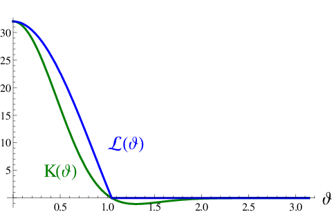
The eigenvalues of the operator are computed to be
showing that the operator is indeed positive. Thus we can apply Proposition 5.3. Using that
we obtain the heat kernel estimate
In this estimate, we are still free to choose the parameters and . By adjusting these parameters, one gets the lower bound shown in Figure 6. Thus the heat kernel estimate differs from the minimal action only by an error of about , and describes the qualitative dependence on quite well. But of course, it does not take into account the discreteness of the minimizers.
6. The Variational Principles on the Flag Manifold
We finally make a few comments on the variational principles on the flag manifold in the case (see Example (c) on page (b)). We first apply our main Theorems 3.16 and 3.18 to obtain the following general result.
Theorem 6.1.
Every minimizer on is either generically timelike or .
Proof.
As a homogeneous space, the flag manifold has a real analytic structure (see [22, Chapter II, §4]). Then the function is obviously real analytic. Moreover, it is symmetric and constant on the diagonal. In order to apply Theorem 3.16, for given we must find a curve joining and which satisfies (3.12). Alternatively, in order to apply Theorem 3.18, our task is to construct a curve with and which is analytic in a neighborhood of , such that the function changes sign at .
We denote the range of by and the orthogonal projection to by . Choosing an orthonormal basis of , the matrix can be represented in terms of Pauli matrices by
Similarly, the operator has the representation
where the real parameters and satisfy the inequalities
Using (1.14), the function is computed by
where denotes the angle between and . The operator has rank two if and only if . A short calculation shows that in this case, has only transverse zeros. Thus we can choose a direction where the condition (3.12) is satisfied. Choosing a smooth curve starting in this direction which joins and , we can apply Theorem 3.16 (A) to conclude the proof in this case.
It remains to consider the situation when has rank at most one. This leads us to several cases. We begin with the case when vanishes. In this case, we may restrict attention to the four-dimensional subspace . In a suitable basis of this subspace, the operators and have the matrix representations
where again . A unitary transformation of the basis vectors and describes a rotation of the vector in . By a suitable transformation of this type, we can arrange that the angle between and equals (see (1.13)). We now define the curve by
| (6.1) |
where is the geodesic on with and . The curve is a real analytic function with and , which is obviously translation symmetric. Furthermore, one computes
where is the corresponding function on the unit sphere (1.12). As changes sign at , the function changes sign at . Thus Theorem 3.18 (A) applies, completing the proof in the case .
We next consider the case that has rank one. We choose the basis of such that is diagonal,
An elementary consideration shows that we can extend the basis of to an orthonormal system such that on the subspace , the operator has the form
| (6.2) |
We let be the unitary transformation
Setting , the matrix becomes
where and are new parameters with
| (6.3) |
and is again a unit vector. The function is now computed by
| (6.4) |
In order to simplify the trace, we transform the phase of . This changes the phase of in (6.2), thus describing a rotation of the vector in the -plane. This makes it possible to arrange that the vectors and are orthogonal in . We thus obtain
We now have two subcases:
- (1)
: We vary the vectors and as functions of such that the above orthogonality relations remain valid and
with free “velocities” and . Since at , we know that
(6.5) A Taylor expansion yields
(6.6) (6.7) As the factor is non-zero in view of (6.3), the linear term (6.6) does not vanish whenever . By suitably adjusting , we can arrange that the square of this linear term compensates the last term in (6.4) (which is also non-zero in view of our assumption ). Next, we know from (6.5) and our assumptions that the term in (6.7) is non-zero. Thus by a suitable choice of , we can give the quadratic term (6.7) any value we want. Taking the square, in (6.4) we get a contribution . Thus the function changes sign. Transforming to a suitable basis where is a fixed matrix, we obtain a curve which is locally translation symmetric. Extending this curve to a smooth curve which joins the point , we can apply Theorem 3.18 (A).
- (2)
: We know that the matrix is diagonal,
Now we keep fixed, while we choose the curve to be a great circle which is inclined to the -plane by an angle , i.e.
Repeating the above calculation leading to (6.6) and (6.7), one sees that we again get a non-zero contribution to of the order . Thus again changes sign, making it possible to apply Theorem 3.18 (A).
It remains to consider the case when vanishes but . A short consideration shows that cannot have rank two. Thus we can choose the orthonormal basis of such that and . By suitably extending this orthonormal system by and , we can arrange that the operator is invariant on the subspace and has the matrix representation
If , we can again work with the curve (6.1). If on the other hand , the operator is invariant on and has the canonical form
Transforming by the unitary matrix
we can arrange that is again of the form (6.2), but now with coefficients depending on . Setting , we can again use the construction after (6.2). This completes the proof. ∎
For sufficiently large , we can rule out one of the cases in Theorem 6.1, showing that the minimizing measures do have a singular support.
Theorem 6.2.
There are no generically timelike minimizers if
The method of proof is to apply Proposition 3.14 (I). In the next two lemmas we verify the necessary assumptions and compute .
Lemma 6.3.
The operator has rank at most .
Proof.
We extend the method used in the proof of [13, Lemma 1.10]. A point is a Hermitian -matrix of rank two, with non-trivial eigenvalues and . Thus we can represent in in bra/ket notation as
where and are the eigenvectors of , normalized such that
A short calculation shows that the non-trivial eigenvalues of the matrix product coincide with the eigenvalues of the -matrix product
Using (1.14), we can thus write the function as
This makes it possible to recover as the “expectation value”
of a suitable matrix , whose block entries are of the form
and the operators permute the factors of the tensor product,
Hence introducing the operator
we find that . This gives the claim. ∎
In view of this lemma, we may decompose in the form (3.7).
Lemma 6.4.
The eigenvalue in the decomposition (3.7) is given by
Proof.
It is most convenient to represent the elements in as
| (6.8) |
where the vectors are orthonormal. Then the normalized volume measure on can be written as
where and denote the Lebesgue measure on , and is the Dirac distribution. The total volume is computed to be
To simplify the calculations, we fix and choose an eigenvector basis of . Then , whereas is again represented in the form (6.8). Then the eigenvalues of the product depend only on the vector components and . More precisely, using (1.14), we obtain
Our task is to compute the integral . In the case , one uses the symmetries to reduce to a lower-dimensional integral,
where is the constant
Carrying out all integrals gives the claim. The proof in the case is similar. ∎
The remaining question is whether generically timelike minimizers exist for small . In the special case , the operator is positive (see [13, Lemma 1.10]), so that Proposition 3.3 or similarly Proposition 3.12 yields that the standard volume measure is a generically timelike minimizer. However, if , these propositions can no longer be used, because the operator fails to be positive:
Lemma 6.5.
If , the operator has negative eigenvalues.
Proof.
Since , it suffices to find two points such that the corresponding Gram matrix is not positive semi-definite. For given we choose the four vectors
(where are the standard basis vectors of ). Taking the representation (6.8), we obtain two points . The corresponding Gram matrix is computed to be
The determinant of this matrix is negative for small . ∎
In this situation, Proposition 3.15 still gives some information on the possible support of generically timelike minimizers. But it remains an open problem whether and under which conditions generically timelike minimizers exist.
Acknowledgments: We would like to thank the referees for valuable comments on the manuscript.
References
- [1] Y. Bernard and F. Finster, On the structure of minimizers of causal variational principles in the non-compact and equivariant settings, arXiv:1205.0403 [math-ph], to appear in Adv. Calc. Var. (2013).
- [2] T. Bröcker and T. tom Dieck, Representations of Compact Lie Groups, Graduate Texts in Mathematics, vol. 98, Springer-Verlag, New York, 1985.
- [3] S. Capet and G. Friesecke, Minimum energy configurations of classical charges: large asymptotics, arXiv:0907.5097 [math.CA], Appl. Math. Res. Express. AMRX (2009), no. 1, 47–73.
- [4] H.T. Croft, K.J. Falconer, and R.K. Guy, Unsolved Problems in Geometry, Problem Books in Mathematics, Springer-Verlag, New York, 1994, Corrected reprint of the 1991 original.
- [5] A. Diethert, F. Finster, and D. Schiefeneder, Fermion systems in discrete space-time exemplifying the spontaneous generation of a causal structure, arXiv:0710.4420 [math-ph], Int. J. Mod. Phys. A 23 (2008), no. 27/28, 4579–4620.
- [6] F. Finster, The continuum limit of a fermion system involving leptons and quarks: Strong, electroweak and gravitational interactions, in preparation.
- [7] by same author, The Principle of the Fermionic Projector, hep-th/0001048, hep-th/0202059, hep-th/0210121, AMS/IP Studies in Advanced Mathematics, vol. 35, American Mathematical Society, Providence, RI, 2006.
- [8] by same author, The principle of the fermionic projector: An approach for quantum gravity?, arXiv:gr-qc/0601128, Quantum Gravity (B. Fauser, J. Tolksdorf, and E. Zeidler, eds.), Birkhäuser Verlag, Basel, 2006, pp. 263–281.
- [9] by same author, Fermion systems in discrete space-time—outer symmetries and spontaneous symmetry breaking, arXiv:math-ph/0601039, Adv. Theor. Math. Phys. 11 (2007), no. 1, 91–146.
- [10] by same author, A variational principle in discrete space-time: Existence of minimizers, arXiv:math-ph/0503069, Calc. Var. Partial Differential Equations 29 (2007), no. 4, 431–453.
- [11] by same author, An action principle for an interacting fermion system and its analysis in the continuum limit, arXiv:0908.1542 [math-ph] (2009).
- [12] by same author, From discrete space-time to Minkowski space: Basic mechanisms, methods and perspectives, arXiv:0712.0685 [math-ph], Quantum Field Theory (B. Fauser, J. Tolksdorf, and E. Zeidler, eds.), Birkhäuser Verlag, 2009, pp. 235–259.
- [13] by same author, Causal variational principles on measure spaces, arXiv:0811.2666 [math-ph], J. Reine Angew. Math. 646 (2010), 141–194.
- [14] by same author, Entanglement and second quantization in the framework of the fermionic projector, arXiv:0911.0076 [math-ph], J. Phys. A: Math. Theor. 43 (2010), 395302.
- [15] by same author, The fermionic projector, entanglement, and the collapse of the wave function, arXiv:1011.2162 [quant-ph], J. Phys.: Conf. Ser. 306 (2011), 012024.
- [16] by same author, A formulation of quantum field theory realizing a sea of interacting Dirac particles, arXiv:0911.2102 [hep-th], Lett. Math. Phys. 97 (2011), no. 2, 165–183.
- [17] by same author, The continuum limit of a fermion system involving neutrinos: Weak and gravitational interactions, arXiv:1211.3351 [math-ph] (2012).
- [18] F. Finster and A. Grotz, A Lorentzian quantum geometry, arXiv:1107.2026 [math-ph], Adv. Theor. Math. Phys. 16 (2012), no. 4, 1197–1290.
- [19] F. Finster, A. Grotz, and D. Schiefeneder, Causal fermion systems: A quantum space-time emerging from an action principle, arXiv:1102.2585 [math-ph], Quantum Field Theory and Gravity (F. Finster, O. Müller, M. Nardmann, J. Tolksdorf, and E. Zeidler, eds.), Birkhäuser Verlag, Basel, 2012, pp. 157–182.
- [20] F. Finster and M. Reintjes, A non-perturbative construction of the fermionic projector on globally hyperbolic manifolds I – Space-times of finite lifetime, arXiv:1301.5420 [math-ph] (2013).
- [21] P.R. Halmos, Measure Theory, Springer, New York, 1974.
- [22] S. Helgason, Differential Geometry, Lie Groups, and Symmetric Spaces, Pure and Applied Mathematics, vol. 80, Academic Press Inc., New York, 1978.
- [23] P.D. Lax, Functional Analysis, Pure and Applied Mathematics (New York), Wiley-Interscience [John Wiley & Sons], New York, 2002.
- [24] E.B. Saff and A.B.J. Kuijlaars, Distributing many points on a sphere, Math. Intelligencer 19 (1997), no. 1, 5–11.
- [25] N.J.A. Sloane, Tables of sphere packings and spherical codes, IEEE Trans. Inform. Theory 27 (1981), no. 3, 327–338.
- [26] A. Sütő, Crystalline ground states for classical particles, arXiv:math-ph/0508004, Phys. Rev. Lett. 95 (2005), 265501.