Sparser Johnson-Lindenstrauss Transforms
Abstract
We give two different and simple constructions for dimensionality reduction in via linear mappings that are sparse: only an -fraction of entries in each column of our embedding matrices are non-zero to achieve distortion with high probability, while still achieving the asymptotically optimal number of rows. These are the first constructions to provide subconstant sparsity for all values of parameters, improving upon previous works of Achlioptas (JCSS 2003) and Dasgupta, Kumar, and Sarlós (STOC 2010). Such distributions can be used to speed up applications where dimensionality reduction is used.
1 Introduction
The Johnson-Lindenstrauss lemma states:
Lemma 1 (JL Lemma [21]).
For any integer , and any , there exists a probability distribution on real matrices for such that for any ,
Proofs of the JL lemma can be found in [1, 6, 7, 13, 14, 17, 21, 23, 28]. The value of in the JL lemma is optimal [20] (also see a later proof in [22]).
The JL lemma is a key ingredient in the JL flattening theorem, which states that any points in Euclidean space can be embedded into dimensions so that all pairwise Euclidean distances are preserved up to . The JL lemma is a useful tool for speeding up solutions to several high-dimensional problems: closest pair, nearest neighbor, diameter, minimum spanning tree, etc. It also speeds up some clustering and string processing algorithms, and can further be used to reduce the amount of storage required to store a dataset, e.g. in streaming algorithms. Recently it has also found applications in approximate numerical algebra problems such as linear regression and low-rank approximation [10, 34]. See [19, 36] for further discussions on applications.
Standard proofs of the JL lemma take a distribution over dense matrices (e.g. i.i.d. Gaussian or Bernoulli entries), and thus performing the embedding naïvely takes time where has non-zero entries. Several works have devised other distributions which give faster embedding times [2, 3, 4, 18, 27, 38], but all these methods require embedding time even for sparse vectors (even when ). This feature is particularly unfortunate in streaming applications, where a vector receives coordinate-wise updates of the form , so that to maintain some linear embedding of we should repeatedly calculate during updates. Since , even the naïve embedding time method is faster than these approaches.
Even aside from streaming applications, several practical situations give rise to vectors with . For example, a common similarity measure for comparing text documents in data mining and information retrieval is cosine similarity [33], which is approximately preserved under any JL embedding. Here, a document is represented as a bag of words with the dimensionality being the size of the lexicon, and we usually would not expect any single document to contain anywhere near distinct words (i.e., we expect sparse vectors). In networking applications, if counts bytes sent from source to destination in some time interval, then is the total number of IP pairs, whereas we would not expect most pairs of IPs to communicate with each other. In linear algebra applications, a rating matrix may for example have as user ’s score for item (e.g. the Netflix matrix where columns correspond to movies), and we would expect that most users rate only small fraction of all available items.
One way to speed up embedding time in the JL lemma for sparse vectors is to devise a distribution over sparse embedding matrices. This was first investigated in [1], which gave a JL distribution where only one third of the entries of each matrix in its support was non-zero, without increasing the number of rows from dense constructions. Later, the works [9, 35] gave a distribution over matrices with only non-zero entries per column, but the algorithm for estimating given the linear sketch then relied on a median calculation, and thus these schemes did not provide an embedding into . In several applications, such as nearest-neighbor search [17] and approximate numerical linear algebra [10, 34], an embedding into a normed space or even itself is required, and thus median estimators cannot be used. Median-based estimators also pose a problem when one wants to learn classifiers in the dimension-reduced space via stochastic gradient descent, since in this case the estimator needs certain differentiability properties [39]. In fact, the work of [39] investigated JL distributions over sparse matrices for this reason, in the context of collaborative spam filtering. The work [12] later analyzed the JL distribution in [39] and showed that it can be realized where for each matrix in the support of the distribution, each column has at most 11 1 We say when , when , and when and simultaneously. non-zero entries, thus speeding up the embedding time to . This “DKS construction” requires bits of random seed to sample a matrix from their distribution. The work of [12] left open two main directions: (1) understand the sparsity parameter that can be achieved in a JL distribution, and (2) devise a sparse JL transform distribution which requires few random bits to sample from, for streaming applications where storing a long random seed requires prohibitively large memory.
The previous work [23] of the current authors made progress on both these questions by showing sparsity was achievable by giving an alternative analysis of the scheme of [12] which also only required seed length. The work of [7] later gave a tighter analysis under the assumption , improving the sparsity and seed length further by and factors in this case. In Section 5 we show that the DKS scheme requires , and thus a departure from their construction is required to obtain better sparsity. For a discussion of other previous work concerning the JL lemma see [23].

|

|
| (a) | (b) |
(c)
Main Contribution:
In this work, we give two new constructions which achieve sparsity for embedding into optimal dimension . This is the first sparsity bound which is always for the asymptotically optimal value of for all ranges of . One of our distributions can be sampled from using uniform random bits.
It is also worth nothing that after the preliminary version of this work was published in [24], it was shown in [32] that our bound is optimal up to an factor. That is, for any fixed constant , any distribution satisfying Lemma 1 that is supported on matrices with and at most non-zero entries per column must have as long as . Note that once one can always take the distribution supported solely on the identity matrix, giving and satisfying Lemma 1 with .
We also describe variations on our constructions which achieve sparsity , but which have much simpler analyses. We describe our simpler constructions in Section 3, and our better constructions in Section 4. We show in Section 5 that our analyses of the required sparsity in our schemes are tight up to a constant factor. In Section 6 we discuss how our new schemes speed up the numerical linear algebra algorithms in [10] for approximate linear regression and best rank- approximation in the streaming model of computation. We also show in Section 6 that a wide range of JL distributions automatically provides sketches for approximate matrix product as defined in [34]. While [34] also showed this, it lost a logarithmic factor in the target dimension due to a union bound in its reduction; the work of [10] avoided this loss, but only for the JL distribution of random sign matrices. We show a simple and general reduction which incurs no loss in parameters. Plugging in our sparse JL transform then yields faster linear algebra algorithms using the same space. In Section 7 we state two open problems for future work.
1.1 Our Approach
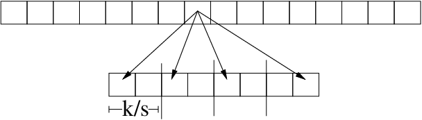
Our constructions are depicted in Figure 1. Figure 1(a) represents the DKS construction of [12] in which each item is hashed to random target coordinates with replacement. Our two schemes achieving are as follows. Construction (b) is much like (a) except that we hash coordinates times without replacement; we call this the graph construction, since hash locations are specified by a bipartite graph with left vertices, right vertices, and left-degree . In (c), the target vector is divided into contiguous blocks each of equal size , and a given coordinate in the original vector is hashed to a random location in each block (essentially this is the CountSketch of [9], though we use a higher degree of independence in our hash functions); we call this the block construction. In all cases (a), (b), and (c), we randomly flip the sign of a coordinate in the original vector and divide by before adding it in any location in the target vector.
We give two different analyses for both our constructions (b) and (c). Since we consider linear embeddings, without loss of generality we can assume , in which case the JL lemma follows by showing that , which is implied by . Thus it suffices to show that for any unit norm ,
| (1) |
We furthermore observe that both our graph and block constructions have the property that the entries of our embedding matrix can be written as
| (2) |
where the are independent and uniform in , and is an indicator random variable for the event (in fact in our analyses we will only need that the are -wise independent). Note that the are not independent, since in both constructions we have that there are exactly non-zero entries per column. Furthermore in the block construction, knowing that for in some block implies that for all other in the same block.
To outline our analyses, look at the random variable
| (3) |
Our proofs all use Markov’s bound on the th moment to give for an even integer. The task is then to bound . In our first approach, we observe that is a quadratic form in the of Eq. (2), and thus its moments can be bounded via the Hanson-Wright inequality [16]. This analysis turns out to reveal that the hashing to coordinates in the target vector need not be done randomly, but can in fact be specified by any sufficiently good code (i.e. the need not be random). Specifically, it suffices that for any , . That is, no two columns have their non-zero entries in more than of the same rows. In (b), this translates to the columns of the embedding matrix (ignoring the random signs and division by ) to be codewords in a constant-weight binary code of weight and minimum distance . In (c), if for each we let be a length- vector with entries in specifying where coordinate is mapped to in each block, it suffices for to be a code of minimum distance . It is fairly easy to see that if one wants a deterministic hash function, it is necessary for the columns of the embedding matrix to be specified by a code: if two coordinates have their non-zeroes in many of the same rows, it means those coordinates collide often. Since collision is the source of error, an adversary in this case could ask to embed a vector which has its mass equally spread on these two coordinates, causing large error with large probability over the choice of random signs. What our analysis shows is that not only is a good code necessary, but it is also sufficient.
In our second analysis approach, we define
| (4) |
so that
| (5) |
We show that to bound it suffices to bound for each . To bound , we expand expand to obtain a polynomial with roughly terms. We view its monomials as being in correspondence with graphs, group monomials that map to the same graph, then do some combinatorics to make the expectation calculation feasible. We remark that a similar tactic of mapping monomials to graphs then carrying out combinatorial arguments is frequently used to analyze the eigenvalue spectrum of random matrices; see for example work of Wigner [40], or the work of Füredi and Komlós [15]. In our approach here, we assume that the random signs as well as the hashing to coordinates in the target vector are done -wise independently. This combinatorial approach of mapping to graphs played a large role in our previous analysis of the DKS construction [23], as well as a later analysis of that construction in [7].
We point out here that Figure 1(c) is somewhat simpler to implement, since there are simple constructions of -wise hash families [8]. Figure 1(b) on the other hand requires hashing without replacement, which amounts to using random permutations and can be derandomized using almost -wise independent permutation families [26] (see Remark 14).
2 Conventions and Notation
Definition 2.
For , the Frobenius norm of is .
Definition 3.
For , the operator norm of is . In the case is symmetric, this is also the largest magnitude of an eigenvalue of .
Henceforth, all logarithms are base- unless explicitly stated otherwise. For a positive integer we use to denote the set . We will always be focused on embedding a vector into , and we assume without loss of generality (since our embeddings are linear). All vectors are assumed to be column vectors, and denotes its transpose. We often implicitly assume that various quantities, such as , are powers of or , which is without loss of generality. Space complexity bounds (as in Section 6), are always measured in bits.
3 Code-Based Constructions
In this section, we provide analyses of our constructions (b) and (c) in Figure 1 when the non-zero entry locations are deterministic but satisfy a certain condition. In particular, in the analysis in this section we assume that for any ,
| (6) |
That is, no two columns have their non-zero entries in more than of the same rows. We show how to use error-correcting codes to ensure Eq. (6) in Remark 8 for the block construction, and in Remark 9 for the graph construction. Unfortunately this step will require setting to be slightly larger than the desired . We give an alternate analysis in Section 4 which avoids assuming Eq. (6) and obtains an improved bound for by not using deterministic .
In what follows, we assume for a sufficiently large constant , and that is some integer dividing satisfying . We also assume that the are -wise independent for , so that is fully determined.
Analysis of Figure 1(b) and Figure 1(c) code-based constructions:
Recall from Eq. (3)
Note is a quadratic form in which can be written as for a block-diagonal matrix . There are blocks, each , where in the th block we have for and for all . Now, . To obtain an upper bound for this probability, we use the Hanson-Wright inequality combined with a Markov bound.
Theorem 4 (Hanson-Wright inequality [16]).
Let be a vector of i.i.d. Rademacher random variables. For any symmetric and ,
for some universal constant independent of .
We prove our construction satisfies the JL lemma by applying Theorem 4 with .
Lemma 5.
.
Lemma 6.
.
Proof. Since is block-diagonal, its eigenvalues are the eigenvalues of each block. For a block , write . is diagonal with , and . Since and are both positive semidefinite, we have . We have . Define by so . Thus .
By Eq. (1), it now suffices to prove the following theorem.
Theorem 7.
.
Proof. By a Markov bound applied to for an even integer,
Since and , applying Theorem 4 with , , and gives
| (7) |
since the th moment is determined by -wise independence of . We conclude the proof by noting that the expression in Eq. (7) is at most for our choices for .
We now discuss how to choose the non-zero locations in to ensure Eq. (6).
Remark 8.
Consider the block construction, and for let specify the locations of the non-zero entries for column of in each of the blocks. Then Eq. (6) is equivalent to being an error-correcting code with relative distance , i.e. that no pair for agree in more than coordinates. It is thus important to know whether such a code exists. Let be such that gives the non-zero location in block for column , i.e. . Note that having relative distance is to say that for every , for at most values of . For let be an indicator random variable for the event , and define . Then , and if , then a Chernoff bound shows that with probability at least over the choice of (in fact it suffices to use Markov’s bound applied to the moment implied by the Chernoff bound so that can be -wise independent, but we do not dwell on this issue here since Section 4 obtains better parameters). Thus by a union bound over all pairs , is a code with the desired properties with probability at least . Note that the condition is equivalent to . We also point out that we may assume without loss of generality that . This is because there exists an embedding into this dimension with sparsity using only -wise independence with distortion and success probability [9, 35]. It is worth noting that in the construction in this section, potentially could be deterministic given an explicit code with our desired parameters.
Remark 9.
It is also possible to use a code to specify the hash locations in the graph construction. In particular, let the th entry of the th column of the embedding matrix be the th symbol of the th codeword (which we call ) in a weight- binary code of minimum distance for . Define for as an indicator variable for . Then, the error is again exactly as in Eq. (3). Also, as in Remark 8, such a code can be shown to exist via the probabilistic method (the Chernoff bound can be applied using negative dependence, followed by a union bound) as long as . We omit the details since Section 4 obtains better parameters.
Remark 10.
Only using Eq. (6), it is impossible to improve our sparsity bound further. For example, consider an instantiation of the block construction in which Eq. (6) is satisfied. Create a new set of which change only in the case so that for all , so that Eq. (6) still holds. In our construction this corresponds to all indices colliding in the first chunk of coordinates, which creates an error term of . Now, suppose consists of entries each with value . Then, with probability , all these entries receive the same sign under and contribute a total error of in the first chunk alone. We thus need , which implies .
4 Random Hashing Constructions
In this section, we show that if the hash functions described in Remark 8 and Remark 9 are not specified by fixed codes, but rather are chosen at random from some family of sufficiently high independence, then one can achieve sparsity (in the case of Figure 1(b), we actually need almost k-wise independent permutations). Recall our bottleneck in reducing the sparsity in Section 3 was actually obtaining the codes, discussed in Remark 8 and Remark 9.
We perform our analysis by bounding the moment of from first principles for an even integer (for this particular scheme, it seems the Hanson-Wright inequality does not simplify any details of the proof). To show Eq. (1) we then use Markov’s inequality to say . Although the are specified differently in the two constructions, in both cases they are easily seen to be negatively correlated; that is, for any subset (in fact in our proof we will only be concerned with ) we have . Also, each construction has with probability for all , and thus, recalling the definition of from Eq. (4),
We first bound the moment of each for . As in the Frobenius norm moment bound of [23], and also used later in [7], the main idea is to construct a correspondence between the monomials appearing in and certain graphs. Notice
| (8) |
To each monomial above we associate a directed multigraph with labeled edges whose vertices correspond to the distinct and . An term corresponds to a directed edge with label from the vertex corresponding to to the vertex corresponding to . The basic idea we use to bound is to group these monomials based on their associated graphs.
Lemma 11.
For an integer, .
Proof. We have
| (9) |
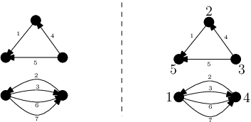
Define as the set of directed multigraphs with edges having distinct labels in and no self-loops, with between and vertices (inclusive), and where every vertex has non-zero and even degree (we use degree to denote the sum of in- and out-degrees). Let map variable sequences to their corresponding graph. That is, we draw a directed edge labeled from the vertex representing to that representing for , where one vertex represents all the which are assigned the same element of (see Figure 2). For a graph , let be its number of vertices, and let be the degree of vertex . By construction every monomial maps to a graph with edges. Also we need only consider graphs with all even vertex degrees since a monomial whose graph has at least one vertex with odd degree will have at least one random sign appearing an odd number of times and thus have expectation zero. Then,
| (10) | ||||
| (11) | ||||
| (12) | ||||
| (13) |
where is the set of all directed multigraphs as in , but in which vertices are labeled as well, with distinct labels in (see Figure 2; the vertex labels can be arbitrarily permuted).
Eq. (10) used that are independent for any . For Eq. (11), note that , and the coefficient of in its expansion for is . Meanwhile, the coefficient of this monomial when summing over all for a particular is at most . For Eq. (12), we move from graphs in to those in , and for any there are exactly ways to label vertices. This is because for any graph there is a canonical way of labeling the vertices as since there are no isolated vertices. Namely, the vertices can be labeled in increasing order of when they are first visited by an edge when processing edges in order of increasing label (if two vertices are both visited for the first time simultaneously by some edge, then we can break ties consistently using the direction of the edge). Thus the vertices are all identified by this canonical labeling, implying that the vertex labelings all give distinct graphs in . Eq. (13) follows since and
The summation over in Eq. (13) is over the with vertices. Let us bound this summation for some fixed choice of vertex degrees . For any given , consider the set of all graphs on labeled vertices with distinct labels in , and with edges with distinct labels in (that is, we do not require even edge degrees, and some vertices may even have degree ). For a graph , let represent the degree of vertex in . For define the function
| (14) |
Let be those graphs with vertices such that vertex has degree . Then
since . To upper bound , note . For , note any graph in can be formed by taking a graph and adding an edge labeled from to for some vertices in . This change causes to both increase by , whereas all other degrees stay the same. Thus considering Eq. (14),
with the last inequality using Cauchy-Schwarz. Thus by induction, . Since , we have . We then have that the summation in Eq. (13) is at most the number of choices of even summing to (there are such choices), times , implying
By differentiation, the quantity is maximized for (recall ), giving our lemma.
Corollary 12.
For an integer, .
Proof. We use Lemma 11. In the case we can multiply the term by and still obtain an upper bound, and in the case of larger we have since . Also when we have , so that .
Theorem 13.
For some , we have .
Proof. We choose an even integer to be specified later. Using Eq. (5) and for all ,
| (15) | ||||
| (16) | ||||
| (17) | ||||
| (18) | ||||
| (19) | ||||
| (20) | ||||
| (21) |
Eq. (15) follows since the expansion of into monomials contains all nonnegative terms, in which the participating terms are negatively correlated, and thus is term-by-term dominated when expanding into a sum of monomials by the case when the are independent. Eq. (16) uses Corollary 12, and Eq. (17) uses . Eq. (18) compares geometric and arithmetic means, giving . Eq. (19) bounds . Eq. (20) follows since there are ways to choose the , and there are at most ways to choose the summing to . Taking derivatives shows that the right hand side of Eq. (21) is maximized for , which will be bigger than and less than by our choices of that will soon be specified. Then gives a summand of . We choose and so that Eq. (21) is at most . Then to ensure we choose . The theorem then follows by Markov’s inequality.
Remark 14.
In order to use fewer random bits to sample from the graph construction, we can use the following implementation. We realize the distribution over via two hash functions and . The function is drawn from from a -wise independent family. The function has the property that for any , exactly distinct have ; in particular, we pick seeds -wise independently to determine for , and where each is drawn from a -almost -wise independent family of permutations on for . The seed length required for any one such permutation is [26], and thus we can pick such seeds -wise independently using total seed length . We then let iff some has . Recall that a -almost -wise independent family of permutations from onto itself is a family of permutations where the image of any fixed elements in has statistical distance at most when choosing a random when compared with choosing a uniformly random permutation . Now, there are monomials in the expansion of . In each such monomial, the coefficient of the term is at most . In the end, we want to apply Markov’s inequality. Thus, we want .
Remark 15.
It is worth noting that if one wants distortion with probability simultaneously for all in some set , our proof of Theorem 13 reveals that it suffices to set and .
5 Tightness of analyses
In this section we show that sparsity is required in Figure 1(b) and Figure 1(c), even if the hash functions used are completely random. We also show that sparsity is required in the DKS construction (Figure 1(a)), nearly matching the upper bounds of [7, 23]. Interestingly, all three of our proofs of (near-)tightness of analyses for these three constructions use the same hard input vectors. In particular, if , then we show that a vector with entries each of value incurs large distortion with large probability. If but is still not sufficiently large, we show that the vector incurs large distortion with large probability (in fact, for the DKS scheme one can even take the vector ).
5.1 Near-tightness for DKS Construction
The main theorem of this section is the following.
Theorem 16.
The DKS construction of [12] requires sparsity to achieve distortion with success probability .
Before proving Theorem 16, we recall the DKS construction (Figure 1(a)). First, we replicate each coordinate times while preserving the norm. That is, we produce the vector , where each is replicated times. Then, pick a random embedding matrix for where each column has exactly one non-zero entry, in a location defined by some random function , and where this non-zero entry is , determined by some random function . The value is some fixed constant. The final embedding is applied to . We are now ready to prove Theorem 16. The proof is similar to that of Theorem 19.
Our proof will use the following standard fact.
Fact 17 ([30, Proposition B.3]).
For all with and ,
Proof (of Theorem 16). First suppose . Consider a vector with non-zero coordinates each of value . If there is exactly one pair that collides under , and furthermore the signs agree under , the norm squared of our embedded vector will be . Since , this quantity is at least . The event of exactly one pair colliding occurs with probability
which is much larger than for smaller than some constant. Now, given a collision, the colliding items have the same sign with probability .
We next consider the case . Consider the vector . If there are exactly three pairs that collide under in three distinct target coodinates, and furthermore the signs agree under , the norm squared of our embedded vector will be . The event of three pairs colliding occurs with probability
which is much larger than for smaller than some constant. Now, given a collision, the colliding items have the same sign with probability .
We lastly consider the case for some constant (depending on ) to be determined later. First note this case only exists when . Define . Suppose there exists an integer so that
- 1.
- 2.
- 3.
.
First we show it is possible to satisfy the above conditions simultaneously for our range of . We set , satisfying item 1 trivially, and item 2 since . For item 3, Fact 17 gives
The term is at least by the settings of , and the term is also at least for sufficiently small.
Now, consider the event that exactly of the copies of are hashed to by , and to by . If occurs, then coordinate in the target vector contributes to in the target vector by item 1 above, whereas these coordinates only contribute to by item 2 above, thus causing error at least . Furthermore, the coordinates which do not hash to are being hashed to a vector of length with random signs, and thus these coordinates have their contribution preserved up to with constant probability by Chebyshev’s inequality. It thus just remains to show that . We have
The term is and thus overall .
5.2 Tightness of Figure 1(b) analysis
Theorem 18.
For smaller than a constant depending on for , the graph construction of Section 4 requires to obtain distortion with probability .
Proof. First suppose . We consider a vector with non-zero coordinates each of value . If there is exactly one set with such that are both non-zero for the embedding matrix (i.e., there is exactly one collision), then the total error is . It just remains to show that this happens with probability larger than . The probability of this occurring is
Now consider the case for some small constant . Consider the vector . Suppose there are exactly collisions, i.e. distinct values of such that are both non-zero (to avoid tedium we disregard floors and ceilings and just assume is an integer). Also, suppose that in each colliding row we have . Then, the total error would be . It just remains to show that this happens with probability larger than . The probability of signs agreeing in exactly chunks is , which is larger than for . The probability of exactly collisions is
| (22) |
It suffices for the right hand side to be at least since is independent of , and thus the total probability of error larger than would be greater than . Taking natural logarithms, it suffices to have
Writing and , the left hand side is . Taking a derivative shows is monotonically increasing for . Thus as long as for a sufficiently small constant , . Also, the term is at most for sufficiently small.
5.3 Tightness of Figure 1(c) analysis
Theorem 19.
For smaller than a constant depending on for , the block construction of Section 4 requires to obtain distortion with probability .
Proof. First suppose . Consider a vector with non-zero coordinates each of value . If there is exactly one set with such that (i.e. exactly one collision), then the total error is . It just remains to show that this happens with probability larger than .
The probability of exactly one collision is
which is larger than for smaller than a universal constant.
Now consider for some small constant . Consider the vector . Suppose there are exactly collisions, i.e. distinct values of such that (to avoid tedium we disregard floors and ceilings and just assume is an integer). Also, suppose that in each colliding chunk we have . Then, the total error would be . It just remains to show that this happens with probability larger than . The probability of signs agreeing in exactly chunks is , which is larger than for . The probability of exactly collisions is
The above is at most , by the analysis following Eq. (22). Since is independent of , the total probability of having error larger than is greater than .
6 Faster numerical linear algebra streaming algorithms
The works of [10, 34] gave algorithms to solve various approximate numerical linear algebra problems given small memory and a only one or few passes over an input matrix. They considered models where one only sees a row or column at a time of some matrix . Another update model considered was the turnstile streaming model. In this model, the matrix starts off as the all zeroes matrix. One then sees a sequence of updates , where each update triggers the change . The goal in all these models is to compute some functions of at the end of seeing all rows, columns, or turnstile updates. The algorithm should use little memory (much less than what is required to store explicitly). Both works [10, 34] solved problems such as approximate linear regression and best rank- approximation by reducing to the problem of sketches for approximate matrix products. Before delving further, first we give a definition.
Definition 20.
Distribution over has -JL moments if for all with ,
Now, the following theorem is a generalization of [10, Theorem 2.1]. The theorem states that any distribution with JL moments also provides a sketch for approximate matrix products. A similar statement was made in [34, Lemma 6], but that statement was slightly weaker in its parameters because it resorted to a union bound, which we avoid by using Minkowski’s inequality.
Theorem 21.
Given , let be any distribution over matrices with columns with the -JL moment property for some . Then for any real matrices with rows,
Proof. Let each have norm . Then
so that, defining (which is a norm for by Minkowski’s inequality),
Now, if has columns and has columns, label the columns of as and the columns of as . Define the random variable . Then . Then again by Minkowski’s inequality since ,
Then by Markov’s inequality and using ,
Remark 22.
Often when one constructs a JL distribution over matrices, it is shown that for all with and for all ,
Any such distribution automatically satisfies the -JL moment property for any by converting the tail bound into a moment bound via integration by parts.
Remark 23.
After this work there was interest in finding sparse oblivious subspace embeddings, i.e. a randomized and sparse such that for any with orthonormal columns, . Here the norm is to operator norm, and thus implies that for all in the column span of . It was shown in [11, 29, 31] that such exists with one non-zero entry per column and rows. It has sinced been pointed out to us by Huy Lê Nguyn that this result also follows from Theorem 21. Indeed, [35] provides a distribution with -JL moments with rows, and supported on matrices each with exactly one non-zero entry per column. The claim then follows by applying Theorem 21 with and by noting that and that operator norm is upper bounded by Frobenius norm.
Now we arrive at the main point of this section. Several algorithms for approximate linear regression and best rank- approximation in [10] simply maintain as is updated, where comes from the JL distribution with -wise independent entries. In fact though, their analyses of their algorithms only use the fact that this distribution satisfies the approximate matrix product sketch guarantees of Theorem 21. Due to Theorem 21 though, we know that any distribution satisfying the -JL moment condition gives an approximate matrix product sketch. Thus, random Bernoulli matrices may be replaced with our sparse JL distributions in this work. We now state some of the algorithmic results given in [10] and describe how our constructions provide improvements in the update time (the time to process new columns, rows, or turnstile updates).
As in [10], when stating our results we will ignore the space and time complexities of storing and evaluating the hash functions in our JL distributions. We discuss this issue later in Remark 26.
6.1 Linear regression
In this problem we have an and . We would like to compute a vector such that with probability . In [10], it is assumed that the entries of require bits of precision to store precisely. Both receive turnstile updates.
Theorem 3.2 of [10] proves that such an can be computed with probability from and , where is drawn from a distribution that simultaneously satisfies both the and -JL moment properties for some fixed constant in their proof, and where . Thus due to Remark 15, we have the following.
Theorem 24.
There is a one-pass streaming algorithm for linear regression in the turnstile model where one maintains a sketch of size . Processing each update requires arithmetic operations and hash function evaluations.
6.2 Low rank approximation
In this problem, we have an of rank with entries that require precision to store. We would like to compute the best rank- approximation to . We define as the error of . We relax the problem by only requiring that we compute a matrix such that with probability over the randomness of the algorithm.
Two-pass algorithm:
Theorem 4.4 of [10] gives a -pass algorithm where in the first pass, one maintains where is drawn from a distribution that simultaneously satisfies both the and -JL moment properties for some fixed constant in their proof. It is also assumed that . The first pass is thus sped up again as in Theorem 24.
One-pass algorithm for column/row-wise updates:
Theorem 4.5 of [10] gives a one-pass algorithm in the case that is seen either one whole column or row at a time. The algorithm maintains both and where is drawn from a distribution that simultaneously satisfies both the and -JL moment properties. This implies the following.
Theorem 25.
There is a one-pass streaming algorithm for approximate low rank approximation with row/column-wise updates where one maintains a sketch of size . Processing each update requires amortized arithmetic operations and hash function evaluations per entry of .
Three-pass algorithm for row-wise updates:
Theorem 4.6 of [10] gives a three-pass algorithm using less space in the case that is seen one row at a time. Again, the first pass simply maintains where is drawn from a distribution that satisfies both the and -JL moment properties. This pass is sped up using our sparser JL distribution.
One-pass algorithm in the turnstile model, bi-criteria:
Theorem 4.7 of [10] gives a one-pass algorithm under turnstile updates where and are maintained in the stream. is drawn from a distribution satisfying both the and -JL moment properties. is drawn from a distribution satisfying both the and -JL moment properties. Theorem 4.7 of [10] then shows how to compute a matrix of rank which achieves the desired error guarantee given and .
One-pass algorithm in the turnstile model:
Theorem 4.9 of [10] gives a one-pass algorithm under turnstile updates where and are maintained in the stream. is drawn from a distribution satisfying both the and -JL moment properties. is drawn from a distribution satisfying both the and -JL moment properties. Theorem 4.9 of [10] then shows how to compute a matrix of rank which achieves the desired error guarantee given and .
Remark 26.
In the algorithms above, we counted the number of hash function evaluations that must be performed. We use our construction in Figure 1(c), which uses -wise independent hash functions. Standard constructions of -wise independent hash functions over universes with elements fitting in a machine word require time to evaluate [8]. In our case, this would blow up our update time by factors such as or , which could be large. Instead, we use fast multipoint evaluation of polynomials. The standard construction [8] of our desired hash functions mapping some domain onto itself for a power of takes a degree- polynomial with random coefficients in . The hash function evaluation at some point is then the evaluation over . Theorem 27 below states that can be evaluated at points in total time . We note that in the theorems above, we are always required to evaluate some -wise independent hash function on many more than points per stream update. Thus, we can group these evaluation points into groups of size then perform fast multipoint evaluation for each group. We borrow this idea from [25], which used it to give a fast algorithm for moment estimation in data streams.
Theorem 27 ([37, Ch. 10]).
Let be a ring, and let be a degree- polynomial. Then, given distinct , all the values can be computed using operations over .
7 Open Problems
In this section we state two explicit open problems. For the first, observe that our graph construction is quite similar to a sparse JL construction of Achlioptas [1]. The work of [1] proposes a random normalized sign matrix where each column has an expected number of non-zero entries, so that in the notation of this work, the are i.i.d. Bernoulli with expectation . Using this construction, [1] was able to achieve without causing to increase over analyses of dense constructions, even by a constant factor. Meanwhile, our graph construction requires that there be exactly non-zero entries per column. This sole change was the reason we were able to obtain better asymptotic bounds on the sparsity of in this work, but in fact we conjecture an even stronger benefit than just asymptotic improvement. The first open problem is to resolve the following conjecture.
Conjecture 28.
Fix a positive integer . For , define as the error random variable when is the sparse construction of [1] with sparsity parameter . Let be similarly defined, but when using our graph construction. Then for any and any , stochastically dominates . That is, for all , , , .
A positive resolution of this conjecture would imply that not only does our graph construction obtain better asymptotic performance than [1], but in fact obtains stronger performance in a very definitive sense.
The second open problem is the following. Recall that the “metric Johnson-Lindenstrauss lemma” [21] states that for any vectors in , there is a linear map into for which preserves all pairwise Euclidean distances of the vectors up to . Lemma 1 implies this metric JL lemma by setting then performing a union bound over all pairwise difference vectors. Alon showed that is necessary [5]. Our work shows that metric JL is also achievable where every column of the embedding matrix has at most non-zeroes, and this is also known to be tight up to an factor [32]. Thus, for metric JL, the lower bounds for both and are off by factors. Meanwhile, for the form of the JL lemma in Lemma 1 where one wants to succeed on any fixed vector with probability (the “distributional JL lemma”), the tight lower bound on of is known [20, 22]. Thus it seems that obtaining lower bounds for distributional JL is an easier task.
Question: Can we obtain a tight lower bound of for distributional JL in the case that , thus removing the factor gap?
Acknowledgments
We thank Venkat Chandar, Venkatesan Guruswami, Swastik Kopparty, and Madhu Sudan for useful discussions about error-correcting codes, David Woodruff for answering several questions about [10], Piotr Indyk and Eric Price for useful comments and discussion, and Mark Rudelson and Dan Spielman for both pointing out the similarity of our proof of Lemma 11 to the types of arguments that are frequently used to analyze the eigenvalue spectrum of random matrices. We thank Huy Lê Nguyn for pointing out Remark 23. We also thank the anonymous referees for many helpful comments.
References
- [1] Dimitris Achlioptas. Database-friendly random projections: Johnson-Lindenstrauss with binary coins. J. Comput. Syst. Sci., 66(4):671–687, 2003.
- [2] Nir Ailon and Bernard Chazelle. The fast Johnson–Lindenstrauss transform and approximate nearest neighbors. SIAM J. Comput., 39(1):302–322, 2009.
- [3] Nir Ailon and Edo Liberty. Fast dimension reduction using Rademacher series on dual BCH codes. Discrete Comput. Geom., 42(4):615–630, 2009.
- [4] Nir Ailon and Edo Liberty. An almost optimal unrestricted fast Johnson-Lindenstrauss transform. ACM Transactions on Algorithms, 9(3):21, 2013.
- [5] Noga Alon. Problems and results in extremal combinatorics I. Discrete Mathematics, 273(1-3):31–53, 2003.
- [6] Rosa I. Arriaga and Santosh Vempala. An algorithmic theory of learning: Robust concepts and random projection. Machine Learning, 63(2):161–182, 2006.
- [7] Vladimir Braverman, Rafail Ostrovsky, and Yuval Rabani. Rademacher chaos, random Eulerian graphs and the sparse Johnson-Lindenstrauss transform. CoRR, abs/1011.2590, 2010.
- [8] J. Lawrence Carter and Mark N. Wegman. Universal classes of hash functions. J. Comput. Syst. Sci., 18(2):143–154, 1979.
- [9] Moses Charikar, Kevin Chen, and Martin Farach-Colton. Finding frequent items in data streams. Theor. Comput. Sci., 312(1):3–15, 2004.
- [10] Kenneth L. Clarkson and David P. Woodruff. Numerical linear algebra in the streaming model. In Proceedings of the 41st ACM Symposium on Theory of Computing (STOC), pages 205–214, 2009.
- [11] Kenneth L. Clarkson and David P. Woodruff. Low rank approximation and regression in input sparsity time. In Proceedings of the 45th ACM Symposium on Theory of Computing (STOC), pages 81–90, 2013.
- [12] Anirban Dasgupta, Ravi Kumar, and Tamás Sarlós. A sparse Johnson-Lindenstrauss transform. In Proceedings of the 42nd ACM Symposium on Theory of Computing (STOC), pages 341–350, 2010.
- [13] Sanjoy Dasgupta and Anupam Gupta. An elementary proof of a theorem of Johnson and Lindenstrauss. Random Struct. Algorithms, 22(1):60–65, 2003.
- [14] Peter Frankl and Hiroshi Maehara. The Johnson-Lindenstrauss lemma and the sphericity of some graphs. J. Comb. Theory. Ser. B, 44(3):355–362, 1988.
- [15] Zoltán Füredi and János Komlós. The eigenvalues of random symmetric matrices. Combinatorica, 1(3):233–241, 1981.
- [16] David Lee Hanson and Farroll Tim Wright. A bound on tail probabilities for quadratic forms in independent random variables. Ann. Math. Statist., 42(3):1079–1083, 1971.
- [17] Sariel Har-Peled, Piotr Indyk, and Rajeev Motwani. Approximate nearest neighbor: Towards removing the curse of dimensionality. Theory of Computing, 8(1):321–350, 2012.
- [18] Aicke Hinrichs and Jan Vybíral. Johnson-Lindenstrauss lemma for circulant matrices. Random Struct. Algorithms, 39(3):391–398, 2011.
- [19] Piotr Indyk. Algorithmic applications of low-distortion geometric embeddings. In Proceedings of the 42nd Annual Symposium on Foundations of Computer Science (FOCS), pages 10–33, 2001.
- [20] T. S. Jayram and David P. Woodruff. Optimal bounds for Johnson-Lindenstrauss transforms and streaming problems with subconstant error. ACM Transactions on Algorithms, 9(3):26, 2013.
- [21] William B. Johnson and Joram Lindenstrauss. Extensions of Lipschitz mappings into a Hilbert space. Contemporary Mathematics, 26:189–206, 1984.
- [22] Daniel M. Kane, Raghu Meka, and Jelani Nelson. Almost optimal explicit Johnson-Lindenstrauss transformations. In Proceedings of the 15th International Workshop on Randomization and Computation (RANDOM), pages 628–639, 2011.
- [23] Daniel M. Kane and Jelani Nelson. A derandomized sparse Johnson-Lindenstrauss transform. CoRR, abs/1006.3585, 2010.
- [24] Daniel M. Kane and Jelani Nelson. Sparser Johnson-Lindenstrauss transforms. In Proceedings of the 23rd Annual ACM-SIAM Symposium on Discrete Algorithms (SODA), pages 1195–1206, 2012.
- [25] Daniel M. Kane, Jelani Nelson, Ely Porat, and David P. Woodruff. Fast moment estimation in data streams in optimal space. In Proceedings of the 43rd ACM Symposium on Theory of Computing (STOC), pages 745–754, 2011.
- [26] Eyal Kaplan, Moni Naor, and Omer Reingold. Derandomized constructions of k-wise (almost) independent permutations. Algorithmica, 55(1):113–133, 2009.
- [27] Felix Krahmer and Rachel Ward. New and improved Johnson-Lindenstrauss embeddings via the Restricted Isometry Property. SIAM J. Math. Anal., 43(3):1269–1281, 2011.
- [28] Jirí Matousek. On variants of the Johnson-Lindenstrauss lemma. Random Struct. Algorithms, 33(2):142–156, 2008.
- [29] Xiangrui Meng and Michael W. Mahoney. Low-distortion subspace embeddings in input-sparsity time and applications to robust linear regression. In Proceedings of the 45th ACM Symposium on Theory of Computing (STOC), pages 91–100, 2013.
- [30] Rajeev Motwani and Prabakar Raghavan. Randomized Algorithms. Cambridge University Press, 1995.
- [31] Jelani Nelson and Huy L. Nguyn. OSNAP: Faster numerical linear algebra algorithms via sparser subspace embeddings. In Proceedings of the 54th Annual IEEE Symposium on Foundations of Computer Science (FOCS), 2013.
- [32] Jelani Nelson and Huy L. Nguyn. Sparsity lower bounds for dimensionality reducing maps. In Proceedings of the 45th ACM Symposium on Theory of Computing (STOC), pages 101–110, 2013.
- [33] Vipin Kumar Pang-Ning Tan, Michael Steinbach. Introduction to Data Mining. Addison-Wesley, 2005.
- [34] Tamás Sarlós. Improved approximation algorithms for large matrices via random projections. In Proceedings of the 47th Annual IEEE Symposium on Foundations of Computer Science (FOCS), pages 143–152, 2006.
- [35] Mikkel Thorup and Yin Zhang. Tabulation-based 5-independent hashing with applications to linear probing and second moment estimation. SIAM J. Comput., 41(2):293–331, 2012.
- [36] Santosh Vempala. The random projection method, volume 65 of DIMACS Series in Discrete Mathematics and Theoretical Computer Science. American Mathematical Society, 2004.
- [37] Joachim von zur Gathen and Jürgen Gerhard. Modern Computer Algebra. Cambridge University Press, 1999.
- [38] Jan Vybíral. A variant of the Johnson-Lindenstrauss lemma for circulant matrices. J. Funct. Anal., 260(4):1096–1105, 2011.
- [39] Kilian Q. Weinberger, Anirban Dasgupta, John Langford, Alexander J. Smola, and Josh Attenberg. Feature hashing for large scale multitask learning. In Proceedings of the 26th Annual International Conference on Machine Learning (ICML), pages 1113–1120, 2009.
- [40] Eugene P. Wigner. Characteristic vectors of bordered matrices with infinite dimensions. Ann. Math., 62:548–564, 1955.