A simple model for high-energy nucleon-nucleon elastic diffraction and exclusive diffractive electroproduction of vector mesons on protons

The aim of this job is the construction of quite a simple phenomenological model which could be applicable to various processes of high energy diffractive scattering. For this purpose we will consider reactions of nucleon-nucleon elastic diffraction and exclusive electroproduction of vector mesons on protons and try to give a simultaneous description of these processes. This will be done in the framework of the Regge-eikonal approach [1] which allows to satisfy the Froissart-Martin bound [2] explicitly. The basis of this approach is the eikonal (impact parameter) representation of the elastic diffractive non-flip scattering amplitude

$$T_{12\to 12}(s,t)=4\pi\lambda^{1/2}(s,m_{1}^{2},m_{2}^{2})\int_{0}^{\infty}db^{2}J_{0}(b\sqrt{-t})\frac{e^{2i\delta_{12\to 12}(s,b)}-1}{2i}\,,$$

(1)

where $s$ is the collision energy squared, $t$ is the transferred 4-momentum squared, $b$ is the impact parameter, $m_{1}$ and $m_{2}$ are the masses of the scattering particles, $\lambda(s,m_{1}^{2},m_{2}^{2})\equiv s^{2}+m_{1}^{4}+m_{2}^{4}-2m_{1}^{2}s-2m_{2}^{2}s-2m_{1}^{2}m_{2}^{2}$, and the eikonal is the sum of single-reggeon exchange terms [1] (for derivation of the eikonal Regge approximation see, also, Appendix):

$$\delta_{12\to 12}(s,b)=\frac{1}{16\pi\lambda^{1/2}(s,m_{1}^{2},m_{2}^{2})}\int_{0}^{\infty}d(-t)J_{0}(b\sqrt{-t})\delta_{12\to 12}(s,t)=\frac{1}{16\pi\lambda^{1/2}(s,m_{1}^{2},m_{2}^{2})}\times$$

$$\times\int_{0}^{\infty}d(-t)J_{0}(b\sqrt{-t})\left\{\sum_{n}\left(i+{\rm tg}\frac{\pi(\alpha_{n}^{+}(t)-1)}{2}\right)\Gamma_{n}^{(1)+}(t)\Gamma_{n}^{(2)+}(t)\left(\frac{s}{s_{0}}\right)^{\alpha_{n}^{+}(t)}\mp\right.$$

(2)

$$\left.\mp\sum_{n}\left(i-{\rm ctg}\frac{\pi(\alpha_{n}^{-}(t)-1)}{2}\right)\Gamma_{n}^{(1)-}(t)\Gamma_{n}^{(2)-}(t)\left(\frac{s}{s_{0}}\right)^{\alpha_{n}^{-}(t)}\right\}\,.$$

Here $\alpha_{n}^{+}(t)$, $\Gamma_{n}^{(i)+}(t)$ and $\alpha_{n}^{-}(t)$, $\Gamma_{n}^{(i)-}(t)$ are $C$-even and $C$-odd Regge trajectories and reggeon form-factors of the scattered particles, $s_{0}\equiv$ 1 GeV², and the sign “$-$” (“$+$”) before $C$-odd contributions corresponds to the particle-particle (particle-antiparticle) scattering.

The practical use of the Regge-eikonal approach is that in the case of high energy diffraction it allows to reduce the unknown function of two variables, $T_{12\to 12}(s,t)$, to a few functions of one dynamical variable $t$ (Regge trajectories and reggeon form-factors) and to make explicit estimations for the high energy evolution of the diffractive pattern. In the following sections we will demonstrate that for various diffractive reactions there exist wide kinematical ranges where for description of cross-sections it is enough to keep only two $C$-even reggeons in the eikonal, pomeron and $f_{2}$-reggeon.

Since the behavior of Regge trajectories and reggeon form-factors at low values of $t$ is still not calculable in the framework of QCD we have to use for them purely phenomenological (test) expressions. But though the main criterion for our choice of such parametrizations is simplicity we should take into account the QCD asymptotic behavior of Regge trajectories at $t\to-\infty$. For example, if we assume that in the limit of large transfers the pomeron exchanges turn into multi-gluon exchanges then (like in QED [3]) we come to [4, 5, 6]

$$\lim_{t\to-\infty}\alpha_{\rm P}(t)=1\,.$$

(3)

In the case of the quark-antiquark pair ($f_{2}$-reggeon, etc.) one obtains [7]

$$\lim_{t\to-\infty}\alpha_{\bar{q}q}(t)\ln^{1/2}(-t)=\sqrt{\frac{32}{11N_{c}-2n_{f}}}=\sqrt{\frac{32}{21}}\;,$$

(4)

where $N_{c}=3$ is the number of colors and $n_{f}=6$ is the full number of quark flavors.

The main feature of the proposed model is the use of universal (“universality” means “uniqueness”, i.e. that corresponding reggeons are the same in applications of the model to various reactions) and essentially nonlinear Regge trajectories with asymptotical behavior satisfying (3), (4).

Thus, for the nucleon-nucleon elastic diffraction we will exploit the following approximation to the eikonal in the momentum representation:

$$\delta(s,t)=\delta_{\rm P}(s,t)+\delta_{f}(s,t)=\left(i+{\rm tg}\frac{\pi(\alpha_{\rm P}(t)-1)}{2}\right){\Gamma^{({\rm pp})}_{\rm P}}^{2}(t)\left(\frac{s}{s_{0}}\right)^{\alpha_{\rm P}(t)}+$$

(5)

$$+\left(i+{\rm tg}\frac{\pi(\alpha_{f}(t)-1)}{2}\right){\Gamma^{({\rm pp})}_{f}}^{2}(t)\left(\frac{s}{s_{0}}\right)^{\alpha_{f}(t)}.$$

For the pomeron and the $f_{2}$-reggeon trajectories we choose the simplest parametrizations¹¹ 1 One should not consider analytical properties of test parametrizations seriously. True Regge trajectories and reggeon form-factors have much more complicated analytical structure. Nevertheless, at negative values of the argument they could be approximated by simple monotonic test functions. satisfying asymptotical conditions (3), (4):

$$\alpha_{\rm P}(t)=1+C_{\rm P}e^{B_{\rm P}t},\;\;\;\alpha_{f}(t)=\sqrt{\frac{32}{21}}\ln^{-1/2}\frac{t_{f}-t}{\Lambda^{2}_{f}}\,.$$

(6)

The reggeon test form-factors are chosen as

$$\Gamma^{({\rm pp})}_{\rm P}(t)=\Gamma^{({\rm pp})}_{\rm P}e^{b^{({\rm pp})}_{\rm P}t},\;\;\;\;\Gamma^{({\rm pp})}_{f}(t)=\Gamma^{({\rm pp})}_{f}e^{b^{({\rm pp})}_{f}t}\,.$$

(7)

To obtain angular distributions one should substitute (6), (7) into (5), then using (2) and (1) calculate the scattering amplitude (integrals are calculated numerically) and substitute it into the expression for the differential cross-section

$$\frac{d\sigma_{el}}{dt}=\frac{|T_{el}(s,t)|^{2}}{16\pi\lambda(s,m_{p}^{2},m_{p}^{2})}\,.$$

(8)

We postpone the discussion of the used parametrizations to the last section and now apply the proposed phenomenological scheme to the description of the elastic nucleon-nucleon diffractive scattering. Here we restrict ourselves by the kinematical range $\sqrt{s}>$ 60 GeV, 0.01 GeV${}^{2}<-t<$ 1.6 GeV². At larger transfers the systematic deviations of the model curves from experimental angular distributions become too large due to the fact that exponential approximations to reggeon form-factors are invalid in the hard scattering region. At $\sqrt{s}<$ 60 GeV the contributions from secondary reggeons ($\omega$, $\rho$, $a$, etc.) have so significant influence on the values of dynamical quantities at low $t$ and in the region of the first dip that they also should not be ignored.²² 2 In fact, relative deviations about even one percent from the experimental data are noticeable in the near-forward scattering vicinity. So, we take into consideration only $pp$-scattering at $\sqrt{s}\approx$ 62 GeV since at such energy the influence of secondary reggeons is minimal in comparison with other ISR data sets, also due to the fact that $C$-odd and $C$-even secondary contributions to the eikonal have opposite signs and compensate one another. And, at last, in the region $\sqrt{-t}<$ 0.1 GeV the interference with Coulomb interaction takes place.

The value of the pomeron intercept can be extracted explicitly from the data on $\gamma^{*}p$ total cross-sections at high photon virtualities and turns out $\approx 1.31$. We will discuss this below in one of the following sections.

For verification of the model we used the set of data on angular distributions collected by J.R. Cudell, A. Lengyel, and E. Martynov at [8]. The original data can also be found at [9]. The data set for $\sqrt{s}=1.96$ TeV is taken from [10]. The results of applying the model to the data are represented in Fig. 1 and Tabs. 1, 2.

Also, in Fig. 1 the total cross-section dependence on the collision energy [11] is given. In particular, $\sigma^{pp}_{tot}$(7 TeV) $\approx$ 110 mb and $\sigma^{pp}_{tot}$(14 TeV) $\approx$ 128 mb.

We will treat exclusive diffractive electroproduction of vector mesons on protons from the standpoint of the vector-dominance model (VDM) [12] where the incoming photon fluctuates into a virtual vector meson which, in turn, scatters from the target proton. According to the so-called hypothesis of $s$-channel helicity conservation (the adequacy of this approximation is confirmed by numerous experimental data on helicity effects [13, 14]) the cross-section of reaction $\gamma^{*}+p\to V+p$ (here $V$ denotes some vector meson) is dominated by the non-flip helicity amplitude which can be represented in the form

$$T^{\lambda}_{\gamma^{*}p\to Vp}(W^{2},t,Q^{2})=\sum_{V^{\prime}}C_{V^{\prime}}^{\lambda}(Q^{2})T^{\lambda}_{V^{\prime*}p\to Vp}(W^{2},t,Q^{2})\,,$$

(9)

where $W$ is the collision energy, $Q^{2}$ is the incoming photon virtuality, $T^{\lambda}_{V^{\prime*}p\to Vp}(W^{2},t,Q^{2})$ is the diffractive hadronic amplitude with Regge-eikonal structure (the applicability of the Regge-eikonal approach to the hadronic reactions with off-shell particles is grounded in [15]), and the sum is taken over all neutral vector mesons. At low $Q^{2}$ the function $C_{V^{\prime}}^{\lambda}(Q^{2})$ behaves like the coefficient of vector dominance (at high $Q^{2}$ the VDM is invalid [13, 14]) dependent on the type of vector meson $V^{\prime}$, helicity $\lambda$, and virtuality $Q^{2}$.

It is known that for small enough values of $t$ the diagonal coupling of vacuum reggeons to hadrons is much stronger than the off-diagonal coupling (for example, elastic proton-proton scattering has a considerably larger cross-section than diffractive excitation of N(1470) in the proton-proton collisions). Hence, in the high-energy range ($W>30$ GeV) where vacuum exchanges exceed the non-vacuum ones the so-called “diagonal approximation” of (9) may be used

$$T^{\lambda}_{\gamma^{*}p\to Vp}(W^{2},t,Q^{2})=C_{V}^{\lambda}(Q^{2})T_{V^{*}p\to Vp}(W^{2},t,Q^{2}).$$

(10)

Here we should note that measurements by ZEUS Collaboration [13, 14] did not reveal patent dependence on $t$ and $W$ of the ratio of differential cross-sections for the cases of longitudinally and transversely polarized incoming photon and this is the reason why we have omitted the superscript $\lambda$ for $T_{V^{*}p\to Vp}(W^{2},t,Q^{2})$ in (10). In other words, we presume that spin phenomena related to the dependence of $T_{V^{*}p\to Vp}(W^{2},t,Q^{2})$ on helicities of incoming and outgoing particles are much more fine effects than diffractive scattering itself and further deal only with amplitude $T_{\gamma^{*}p\to Vp}(W^{2},t,Q^{2})$ averaged over spin states (it is obtained by the replacement $C_{V}^{\lambda}(Q^{2})\to\sqrt{\frac{1}{3}\sum_{\lambda}{[C_{V}^{\lambda}(Q^{2})]}^{2}}$ in (10)).³³ 3 The $Q^{2}$-behavior of $C_{V}^{\lambda}(Q^{2})$ differs at different $\lambda$ but in this job we concentrate on the reggeon structure of the amplitude and, so, on the helicity independent $W$- and $t$-behavior of cross-sections. For this quantity the extended (off-shell) eikonal representation is valid [15]:

$$T_{\gamma^{*}p\to Vp}(W^{2},b,Q^{2})=\frac{\delta_{\gamma^{*}p\to Vp}(W^{2},b,Q^{2})}{\delta_{Vp\to Vp}(W^{2},b)}T_{Vp\to Vp}(W^{2},b)=$$

(11)

$$=\delta_{\gamma^{*}p\to Vp}(W^{2},b,Q^{2})+i\delta_{\gamma^{*}p\to Vp}(W^{2},b,Q^{2})\delta_{Vp\to Vp}(W^{2},b)+...$$

(where $b$ is the impact parameter, $\delta_{\gamma^{*}p\to Vp}(W^{2},b,Q^{2})$ is the “eikonal” (the sum of pole terms) of the vector meson electroproduction on protons, $\delta_{Vp\to Vp}(W^{2},b)$ is the eikonal of the vector meson elastic scattering on protons, and $T_{Vp\to Vp}(W^{2},b)=\frac{e^{2i\delta_{Vp\to Vp}(W^{2},b)}-1}{2i}$ is the “eikonalized” (unitarized) amplitude of elastic $Vp$-scattering).

The secondary reggeon exchanges are suppressed ($C$-odd reggeon exchanges – due to the $C$-parity conservation, $a_{2}$-reggeon exchange – due to the isospin conservation). Hence, the pole part of the amplitude takes a relatively simple form:

$$\delta_{\gamma^{*}p\to Vp}(W^{2},t,Q^{2})=\left[\left(i+{\rm tg}\frac{\pi(\alpha_{\rm P}(t)-1)}{2}\right)\Gamma^{({\rm V^{*}V})}_{\rm P}(t,Q^{2})\Gamma^{({\rm pp})}_{\rm P}(t)\left(\frac{W^{2}}{W_{0}^{2}}\right)^{\alpha_{\rm P}(t)}+\right.$$

(12)

$$\left.+\left(i+{\rm tg}\frac{\pi(\alpha_{f}(t)-1)}{2}\right)\Gamma^{({\rm V^{*}V})}_{f}(t,Q^{2})\Gamma^{({\rm pp})}_{f}(t)\left(\frac{W^{2}}{W_{0}^{2}}\right)^{\alpha_{f}(t)}\right]\sqrt{\frac{3\Gamma_{V\to e^{+}e^{-}}}{\alpha_{e}M_{V}}}\frac{M^{2}_{V}}{M^{2}_{V}+Q^{2}}\;,$$

where $M_{V}$ is the vector meson mass, $\alpha_{e}\approx\frac{1}{137}$ is the electromagnetic coupling, $\Gamma_{V\to e^{+}e^{-}}$ is the width of the vector meson decay to the electron-positron pair, $W_{0}\equiv 1$ GeV, $\alpha_{\rm P}(t)$ and $\alpha_{f}(t)$ are the pomeron and the $f_{2}$-reggeon trajectories, $\Gamma^{({\rm pp})}_{\rm P}(t)$ and $\Gamma^{({\rm pp})}_{f}(t)$ are the corresponding reggeon form-factors of the proton (the factor $\sqrt{\frac{3\Gamma_{V\to e^{+}e^{-}}}{\alpha_{e}M_{V}}}\frac{M^{2}_{V}}{M^{2}_{V}+Q^{2}}$ is singled out explicitly from the photon-meson-reggeon vertex functions for convenience).

The VDM implies that $\Gamma^{({\rm V^{*}V})}_{\rm R}(t,-M_{V}^{2})=\Gamma^{({\rm V\,V})}_{\rm R}(t)$, where $\Gamma^{({\rm V\,V})}_{\rm R}(t)$ is the reggeon (${\rm R}={\rm P},f$) form-factor of the vector meson:

$$\delta_{Vp\to Vp}(W^{2},t)=\left(i+{\rm tg}\frac{\pi(\alpha_{\rm P}(t)-1)}{2}\right)\Gamma^{({\rm V\,V})}_{\rm P}(t)\Gamma^{({\rm pp})}_{\rm P}(t)\left(\frac{W^{2}}{W_{0}^{2}}\right)^{\alpha_{\rm P}(t)}$$

$$\left(i+{\rm tg}\frac{\pi(\alpha_{f}(t)-1)}{2}\right)\Gamma^{({\rm V\,V})}_{f}(t)\Gamma^{({\rm pp})}_{f}(t)\left(\frac{W^{2}}{W_{0}^{2}}\right)^{\alpha_{f}(t)}.$$

(13)

To calculate $T_{\gamma^{*}p\to Vp}(W^{2},t,Q^{2})$ we should determine functions $\Gamma^{({\rm V^{*}V})}_{\rm R}(t,Q^{2})$ and $\Gamma^{({\rm V\,V})}_{\rm R}(t)$ (functions $\alpha_{\rm R}(t)$ and $\Gamma^{({\rm pp})}_{\rm R}(t)$ were fixed under consideration of elastic nucleon-nucleon scattering).

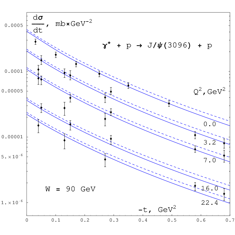
Here we make an assumption that in the diffraction region one can neglect the $t$-dependence of reggeon form-factors of vector mesons (i.e. at low enough values of $t$ the approximations $\Gamma^{({\rm V^{*}V})}_{\rm R}(t,Q^{2})\approx\Gamma^{({\rm V^{*}V})}_{\rm R}(Q^{2})$ and $\Gamma^{({\rm V\,V})}_{\rm R}(t)\approx\Gamma^{({\rm V\,V})}_{\rm R}$ are valid⁴⁴ 4 The hypothesis about the weak $t$-dependence of vector meson reggeon form-factors (in comparison with corresponding form-factors of the proton) is confirmed a posteriori under describing the experimental data.). Such a behavior corresponds to the small effective radii of vector meson interaction with reggeons. According to the dimensional counting rules [16], the quantities $\Gamma^{({\rm V^{*}V})}_{\rm R}(Q^{2})$ should exhibit slow (nonpower-like) $Q^{2}$-behavior (power-like $Q^{2}$-dependence was already singled out above). Taking into account this slow $Q^{2}$-evolution we, also, assume that $\Gamma^{({\rm V\,V})}_{\rm R}\approx\Gamma^{({\rm V^{*}V})}_{\rm R}(0)$ (since we have no possibility to fix the on-shell form-factors separately from the elastic scattering of vector mesons on protons). Thus, for estimation of the photoproduction ($Q^{2}\approx 0$) amplitude we need to determine only two extra free parameters, $\Gamma^{({\rm V^{*}V})}_{\rm P}(0)$ and $\Gamma^{({\rm V^{*}V})}_{f}(0)$.

Applying the model to the data on the photoproduction of $J/\psi(3096)$ on protons [17] yields $\chi^{2}\approx 158$ over 114 points (see Fig. 2).

For the electroproduction of $J/\psi(3096)$ [13, 17] and exclusive production of light vector mesons [18, 14] we obtain rather slow changing of reggeon form-factors with $Q^{2}$ growth (see Figs. 3,4,5⁵⁵ 5 Integrated cross-sections are obtained by integration of the differential ones over $0<-t<1$ GeV² for heavy mesons and over $0<-t<0.6$ GeV² for light mesons. and Tab. 3) in accordance with the dimensional counting rules [16].

For the photoproduction of $\psi(2s)$ [19] and $\Upsilon(1s)$ [20] we obtain $\Gamma^{({\rm\psi^{*}\psi})}_{\rm P}(0)\approx 0.25$, $\Gamma^{({\rm\psi^{*}\psi})}_{f}(0)\approx 0.1$ and $\Gamma^{({\rm\Upsilon^{*}\Upsilon})}_{\rm P}(0)\approx 0.08$, $\Gamma^{({\rm\Upsilon^{*}\Upsilon})}_{f}(0)\approx 0$ (see Fig. 6).

In this section we consider the $W$-behavior of the $\gamma^{*}p$ total cross-sections which are closely related to the proton structure function $F_{2}(x,Q^{2})$ [21]:

$$\sigma^{\gamma^{*}p}_{tot}(W^{2},Q^{2})=\frac{4\pi^{2}\alpha_{e}}{Q^{4}}\frac{Q^{2}+4m_{p}^{2}x^{2}}{1-x}F_{2}(x,Q^{2})\;\;\;\left(x=\frac{Q^{2}}{W^{2}+Q^{2}-m_{p}^{2}}\right)\,.$$

(14)

Following the VDM the non-flip forward $\gamma^{*}p$ scattering amplitude can be represented in the form:

$$T^{\lambda}_{\gamma^{*}p\to\gamma^{*}p}(W^{2},t=0,Q^{2})=\sum_{V^{\prime},V}C_{V^{\prime}}^{\lambda}(Q^{2})T_{V^{\prime*}p\to V^{*}p}(W^{2},t=0,Q^{2})C_{V}^{\lambda}(Q^{2})\,.$$

(15)

Owing to the optical theorem [1] the total cross-section is proportional to the imaginary part of the forward amplitude. From the reggeonic point of view one could single out (at high $W$) the pomeron pole contribution:

$$\sigma^{\gamma^{*}p}_{tot}(W^{2},Q^{2})=\Gamma^{(\gamma^{*}\gamma^{*})}_{\rm P}(Q^{2})\Gamma^{({\rm pp})}_{\rm P}(0)W^{2(\alpha_{\rm P}(0)-1)}+S+A\,,$$

(16)

where $S$ denotes the sum of other pole contributions, $A$ denotes absorptive corrections, and $\Gamma^{(\gamma^{*}\gamma^{*})}_{\rm P}(Q^{2})$ is the pomeron form-factor of virtual photon.

Immediately, a question emerges if there exists such a kinematical range at HERA energies where $S$ and $A$ are negligible and, hence, the simple pole approximation is valid ($W_{0}\equiv 1$ GeV):

$$\sigma^{\gamma^{*}p}_{tot}(W^{2},Q^{2})\approx\beta(Q^{2})\left(\frac{W}{W_{0}}\right)^{2\delta}\,,$$

(17)

where $\beta(Q^{2})\equiv W_{0}^{-2}\Gamma^{(\gamma^{*}\gamma^{*})}_{\rm P}(Q^{2})\Gamma^{({\rm pp})}_{\rm P}(0)$, $\delta\equiv\alpha_{\rm P}(0)-1$.

Such a range exists. At 50 GeV $<W<$ 300 GeV and 25 GeV${}^{2}<Q^{2}\ll W^{2}$ the $W$-behavior of the $\gamma^{*}p$ total cross-sections can be well-described by (17) with $\delta\approx 0.31$ and values of $\beta(Q^{2})$ from Tab. 4 (see Fig. 7).

The slower rising of total cross-sections with the collision energy growth at lower $Q^{2}$ and $W$ is due to the influence of secondary poles and absorptive corrections (the secondary pole terms rise cross-sections at lower energies and absorptive corrections drop them at higher energies). The fact that these contributions are negligibly small in the above-mentioned kinematical range could be explained by the following. Owing to the presence of factors $\frac{M_{V}^{2}}{M_{V}^{2}+Q^{2}}$ in coefficients $C_{V}^{\lambda}(Q^{2})$, at high photon virtualities the scattering amplitude (15) is dominated by fluctuations to heavy vector mesons. But for heavy mesons diffractive scattering the secondary pole terms and the absorptive corrections are suppressed by the pomeron pole term due to the much smaller $f_{2}$-reggeon form-factors (in comparison with both the $f_{2}$-reggeon form-factors of light mesons and the pomeron form-factors) and significantly lower values of the pomeron form-factors. This can be traced explicitly by the collation of the light meson ($\rho^{0}(770)$, $\phi(1020)$) versus the heavy meson ($J/\psi(3096)$, $\psi(2s)$, $\Upsilon(1s)$) exclusive production (see the previous section).

After the extraction of $\delta$ from the data on $F_{2}(x,Q^{2})$ and fixing the pomeron intercept we obtain (see the previous sections) a consistent phenomenological scheme for various exclusive diffractive reactions $2\to 2$ at high energies.

Now let us turn to the general discussion of the proposed model.

One of the advantages of Regge-eikonal approach is that it allows explicit taking into account absorptive corrections. Above there was demonstrated that absorptive corrections are not negligible for elastic nucleon-nucleon scattering and exclusive electroproduction of light vector mesons (see dashed lines in Figs. 1 – 5).

Regge trajectories in our model turn out essentially nonlinear in the diffraction region (see Fig. 1). At first sight such a picture may seem strange but such a nonlinearity is the only way for true Regge trajectories to combine the asymptotic behavior (3), (4) with the approximate large-slope linearity in the resonance region⁶⁶ 6 The resonance masses are determined from equations like $\alpha(M^{2}-{\rm i}M\Gamma)=J$ (here $\alpha(t)$ is some Regge trajectory and $J$ is the resonance spin) which do not imply that ${\rm Re}\,\alpha(M^{2})=J$ and ${\rm Im}\,\alpha(M^{2})=0$. The decay widths $\Gamma$ are only few times less than the corresponding masses $M$: for example, for $f_{2}(1270)$-meson $\frac{\Gamma_{f}}{M_{f}}\approx 0.15$. Consequently, Chew-Frautschi plots should be considered only as very rough approximations to the true Regge trajectories in the resonance region. (observed in the light meson spectroscopy data) and the monotony at negative values of the argument (see Fig. 8). This monotony itself seems quite natural. If ${\rm Im}\,\alpha(t+i0)\geq 0$ increases slowly enough at $t\to+\infty$ (for example, not faster than $Ct\ln^{-1-\epsilon}t$, $\epsilon>0$), the dispersion relations with not more than one subtraction take place, i.e.

$$\alpha(t)=\alpha_{0}+\frac{t}{\pi}\int_{t_{T}}^{+\infty}\frac{{\rm Im}\,\alpha(t^{\prime}+i0)}{t^{\prime}(t^{\prime}-t)}dt^{\prime}\,.$$

And if, in addition, we assume that ${\rm Im}\,\alpha(t+i0)\geq 0$ at $t\geq t_{T}>0$ (we would like to point out that these assumptions are strictly fulfilled in the theory of perturbations and the theory of potential scattering [1]) then

$$\frac{d^{n}\alpha(t)}{dt^{n}}>0\;\;(t<t_{T},\;n=1,2,3,...).$$

Also, using the nonlinear trajectories (instead of linear ones) allows to avoid emerging unphysical singularities in the real part of the signature factors at those points where Regge trajectories take on a value of negative integers.

The eikonal (5) could be called “minimal” since it contains contributions from only those reggeons which are essential for all considered diffractive reactions. For Regge trajectories and reggeon form-factors we chose parametrizations as simple as possible. Expressions (6), (7) were not derived from QCD or general principles. So, they should be considered not as analytic but only as purely quantitative (test) approximations to the true Regge trajectories and reggeon form-factors at negative values of the argument. They are not valid at $t>0$. Moreover, we do not expect that exponential approximations (7) to reggeon form-factors are valid in the region of transfers essentially larger than 1 GeV (exponential form-factors correspond to Gaussian distribution of strongly interacting matter in nucleons). The imperfectness of these approximations and the neglection of secondary reggeons ($\omega$, $\rho$, $a$, etc.) are the causes of systematic deviations of the model curves from the experimental data. Therefore, we had to consider only that kinematical range for the elastic nucleon-nucleon scattering where the contributions from secondary reggeons are small enough and where the non-exponential behavior of reggeon form-factors at high transfers is not essential.

For better description of the considered data sets on nucleon-nucleon scattering and for extension of the model to higher transfers one should use more complicated expressions for the reggeon form-factors. Also, for extension to lower energies and for description of the difference between $pp$ and $\bar{p}p$ cross-sections it is necessary to include secondary reggeons ($\omega$, $\rho$, $a$, etc.) and, possibly, odderon (which could have some influence on the behavior in the dip region). But in this job we deliberately restricted ourselves by the simplest eikonal and the simplest test parametrizations to make the main conclusions more transparent:

• •

  For various diffractive processes there exist wide kinematical ranges where the cross-sections are dominated by only two reggeons, the pomeron and the $f_{2}$-reggeon.

• •

  Regge trajectories are universal in all diffractive reactions⁷⁷ 7 This universality is closely related to the fact that Regge trajectories are analytic (i.e. unique) continuations of observable spectra of resonances. and essentially nonlinear (such a nonlinearity does not contradict to both the phenomenology and the QCD asymptotic relations).

• •

  The pomeron trajectory has intercept $\approx 1.31$ (which could be extracted from the data on the proton structure function $F_{2}(x,Q^{2})$) and corresponds to the so-called “hard” pomeron frequently mentioned in literature. The $f_{2}$-reggeon has intercept $\approx 1.07$ and corresponds to the so-called “soft” pomeron.

• •

  Different cross-section growth rates for various reactions (at high energies) are due to different relative contributions of the $f_{2}$-reggeon to the eikonal.

Among other models for elastic diffractive scattering [22, 23, 24, 25, 26, 27] and exclusive electroproduction of vector mesons [28, 29, 30, 31, 32] the proposed phenomenological scheme stands out due to its salient simplicity and physical clearness and, also, due to the fact that it is the only model which allows to give a simultaneous qualitative description to both “soft” and “hard” exclusive diffractive processes. The range of validity of the model is wide enough to give a good ground for making well-reasoned predictions for elastic diffraction at LHC energies (see Fig. 1). The TOTEM measurements [33] on $pp$ total cross-sections and angular distributions should discriminate among different models.

The obtained approximations to leading vacuum Regge trajectories and reggeon form-factors of the proton could be used under considering more complicated (than $2\to 2$) diffractive reactions: single diffraction ($p+p\to p+X$ or $\bar{p}+p\to\bar{p}+X$), central exclusive diffractive production of the Higgs boson ($p+p\to p+H+p$), etc.

The author is grateful to V.A. Petrov for encouragement and numerous discussions and A.K. Likhoded, G.P. Pronko, V.V. Kiselev, and Yu.F. Pirogov for discussion and useful criticism.

The eikonal representation of the scattering amplitude itself does not yield any progress in solving the problem since it is reduced to the replacement of the unknown function of two variables, $T(s,t)$, to another one, $\delta(s,t)$, without any specification of the functional form of $\delta(s,t)$. The key assumption is that the eikonal is proportional (with high accuracy) to the effective relativistic (quasi-)potential of hadronic interaction. According to the Van Hove interpretation [34] of the relativistic (quasi-)potential as the “sum” over all single-particle exchanges in the $t$-channel, the eikonal can be represented in the form

$$\delta^{(f_{1},f_{2})}(s,t)=\sum_{j=0}^{\infty}\sum_{m_{j}}J^{(f_{1},j,m_{j})}_{\alpha_{1}...\alpha_{j}}(p_{1},\Delta)\frac{D_{(j,m_{j})}^{\alpha_{1}...\alpha_{j},\beta_{1}...\beta_{j}}(\Delta)}{m_{j}^{2}-\Delta^{2}}J^{(f_{2},j,m_{j})}_{\beta_{1}...\beta_{j}}(p_{2},\Delta)\,,$$

$(A.1)$

(here $\frac{D_{(j,m_{j})}^{\alpha_{1}...\alpha_{j},\beta_{1}...\beta_{j}}}{m_{j}^{2}-\Delta^{2}}$ is the propagator of the spin-$j$ particle with mass $m_{j}$, $J^{(f,j,m_{j})}_{\alpha_{1}...\alpha_{j}}$ is the hadronic current (index $f$ denotes the kind of scattering particle), $\Delta$ is the transferred 4-momentums, $t=\Delta^{2}$, $p_{1}$ and $p_{2}$ are 4-momentumes of the incoming hadrons, $s=(p_{1}+p_{2})^{2}$, the symbol $\sum_{m_{j}}$ denotes summing over all spin-$j$ particles with different masses, which, in what further, will be transformed into summing over reggeons). We impose the following constraints on the general dependence of hadronic currents on $\Delta$: symmetry with respect to all $\alpha_{k}$, transversality with respect to $\Delta_{\alpha_{k}}$ ($k=1,...,j$), and tracelessness with respect to any pair of Lorentz indices. The first two conditions yield

$$J^{(f,j,m_{j})}_{\alpha_{1}...\alpha_{j}}(p,\Delta)=\sum_{k=0}^{\left[\frac{j}{2}\right]}\Gamma^{(f,j,m_{j})}_{k}(p^{2},\Delta^{2},(p\Delta))\sum G_{\alpha_{\mu_{1}}\alpha_{\mu_{2}}}...G_{\alpha_{\mu_{2k-1}}\alpha_{\mu_{2k}}}P_{\alpha_{\mu_{k+1}}}...P_{\alpha_{\mu_{j}}},$$

$(A.2)$

where $\Gamma^{(f,j,m_{j})}_{k}(p^{2},\Delta^{2},(p\Delta))$ are some scalar functions, $P_{\alpha}\equiv\frac{p_{\alpha}-\frac{p\Delta}{\Delta^{2}}\Delta_{\alpha}}{\sqrt{p^{2}-\frac{(p\Delta)^{2}}{\Delta^{2}}}}$, $G_{\alpha\beta}\equiv-g_{\alpha\beta}+\frac{\Delta_{\alpha}\Delta_{\beta}}{\Delta^{2}}$, and the inner sum is over all nonequivalent permutations of Lorentz indices (the total number of terms is $\frac{j!}{(2k)!!(j-2k)!}$). Taking into account that

$$g^{\alpha\beta}G_{\alpha\beta}=-3\,,\;\;\;P_{\alpha}P^{\alpha}=1\,,\;\;\;g^{\alpha\beta}G_{\alpha\gamma}G_{\beta\delta}=-G_{\gamma\delta}\,,\;\;\;G_{\alpha\beta}P^{\beta}=-P_{\alpha}\,,$$

$(A.3)$

the tracelessness condition results in the recurrent relations

$$\Gamma^{(f,j,m_{j})}_{k}(p^{2},\Delta^{2},(p\Delta))=\frac{\Gamma^{(f,j,m_{j})}_{k-1}(p^{2},\Delta^{2},(p\Delta))}{2(j-k)+1}\,,$$

$(A.4)$

and, consequently, yields

$$J^{(f,j,m_{j})}_{\alpha_{1}...\alpha_{j}}(p,\Delta)=\Gamma^{(f,j,m_{j})}_{0}(p^{2},\Delta^{2},(p\Delta))\times$$

$(A.5)$

$$\times\sum_{k=0}^{\left[\frac{j}{2}\right]}\frac{(2(j-k)-1)!!}{(2j-1)!!}\sum G_{\alpha_{\mu_{1}}\alpha_{\mu_{2}}}...G_{\alpha_{\mu_{2k-1}}\alpha_{\mu_{2k}}}P_{\alpha_{\mu_{k+1}}}...P_{\alpha_{\mu_{j}}}\,.$$

Substituting (A.5) into (A.1) and taking into account the transversality and the tracelessness of hadronic currents, we come to the following expression for the eikonal:

$$\delta^{(f_{1},f_{2})}(s,t)=\sum_{j=0}^{\infty}\sum_{m_{j}}\frac{\gamma^{(f_{1},f_{2},j,m_{j})}(\Delta^{2})}{m_{j}^{2}-\Delta^{2}}\frac{2^{j}(j!)^{2}}{(2j)!}P_{j}\left(\frac{p_{1}p_{2}-\frac{(p_{1}\Delta)(p_{2}\Delta)}{\Delta^{2}}}{\sqrt{(p_{1}^{2}-\frac{(p_{1}\Delta)^{2}}{\Delta^{2}})(p_{2}^{2}-\frac{(p_{2}\Delta)^{2}}{\Delta^{2}})}}\right),$$

$(A.6)$

where $P_{j}(x)$ are Legendre polynomials of power $j$ and

$$\gamma^{(f_{1},f_{2},j,m_{j})}(\Delta^{2})\equiv\Gamma^{(f_{1},j,m_{j})}_{0}(p_{1}^{2},\Delta^{2},(p_{1}\Delta))\Gamma^{(f_{2},j,m_{j})}_{0}(p_{2}^{2},\Delta^{2},(p_{2}\Delta))\,.$$

$(A.7)$

For elastic scattering we have

$$(p_{1}-\Delta)^{2}=p_{1}^{2}=m_{1}^{2}\,,\;\;\;(p_{2}+\Delta)^{2}=p_{2}^{2}=m_{2}^{2}\,,$$

$(A.8)$

and, so, using the kinematical relations

$$p_{1,2}\Delta=\pm\frac{\Delta^{2}}{2}\,,\;\;\;\;p_{1}p_{2}=\frac{s-m_{1}^{2}-m_{2}^{2}}{2}\,,\;\;\;\;\Delta^{2}\equiv t\,,$$

$(A.9)$

we can simplify the expression for the eikonal (from now on, indices $f_{1}$ and $f_{2}$, denoting the kinds of scattering particles, will be omitted):

$$\delta(s,t)=\sum_{j=0}^{\infty}\sum_{m_{j}}\frac{\gamma^{(j,m_{j})}(t)}{m_{j}^{2}-t}\frac{2^{j}(j!)^{2}}{(2j)!}P_{j}\left(\frac{s-m_{1}^{2}-m_{2}^{2}+\frac{t}{2}}{2\sqrt{(m_{1}^{2}-\frac{t}{4})(m_{2}^{2}-\frac{t}{4})}}\right)\,.$$

$(A.10)$

Here we divide the sum over $j$ in the right-hand side of (A.10) into two sums over even and odd $j$:

$$\delta(s,t)=\delta^{+}(s,t)+\delta^{-}(s,t)=\sum_{j=0}^{\infty}\sum_{\eta=\pm 1}\sum_{m_{(\eta)j}}\frac{\eta+e^{-i\pi j}}{2}(-1)^{j}\frac{\gamma^{(\eta,j,m_{(\eta)j})}(t)}{m_{(\eta)j}^{2}-t}\times$$

$(A.11)$

$$\times\frac{2^{j}(j!)^{2}}{(2j)!}P_{j}\left(\frac{s-m_{1}^{2}-m_{2}^{2}+\frac{t}{2}}{2\sqrt{(m_{1}^{2}-\frac{t}{4})(m_{2}^{2}-\frac{t}{4})}}\right)\,.$$

Each of sequences $\gamma^{(\eta,j,m_{(\eta)j})}(t)$, $m_{(\eta)j}^{2}$ ($j=0,2,4,...,2n,...$ at $\eta=+1$ and $j=1,3,4,...,2n-1,...$ at $\eta=-1$) separately satisfies the conditions of the Carlson theorem [1, 35] which states that if for some analytic and regular at ${\rm Re}\,x\geq 0$ function $f(x)$ the inequality $f(x)<e^{k|x|}$ at some $k<\pi$ is valid, then this function is determined unilocally by its values at integer $x$.

Now we make a key assumption about the possibility of unilocal (under the Carlson theorem) analytic continuation of (A.11) into the region of complex $j$ (the Regge hypothesis [1]). It implies that $m_{(\eta)j}^{2}$ and $\gamma^{(\eta,j,m_{(\eta)j})}(t)$ in (A.11) are the values of analytic (holomorphic with respect to the complex variable $j$) functions for integer non-negative values of $j$. We denote these functions by $m_{\eta}^{2}(j)$ and $\gamma^{(\eta)}(t,j,m_{\eta}^{2}(j))$, respectively. Via the Sommerfeld–Watson transform [1, 36] we replace the sum over $j$ in (A.11) by the integral over the contour $C$ (on the complex plane of the variable $j$) encircling the real positive half-axis including the point $j=0$ in such a way that the half-axis is on the right:

$$\delta(s,t)=\frac{1}{2i}\oint_{C}\frac{dj}{\sin(\pi j)}\sum_{\eta=\pm 1}\sum_{m_{\eta}}\left(-\frac{\eta+e^{-i\pi j}}{2}\right)\frac{\gamma^{(\eta)}(t,j,m_{\eta}^{2}(j))}{m_{\eta}^{2}(j)-t}\times$$

$(A.12)$

$$\times\frac{2^{j}\Gamma^{2}(j+1)}{\Gamma(2j+1)}P\left(j\;,\;\frac{s-m_{1}^{2}-m_{2}^{2}+\frac{t}{2}}{2\sqrt{(m_{1}^{2}-\frac{t}{4})(m_{2}^{2}-\frac{t}{4})}}\right)$$

(here $P(j,x)$ is the analytic continuation of Legendre polynomials $P_{j}(x)$ to the region of complex $j$ and $\Gamma(j)$ is the Euler gamma-function). Since (according to our assumption) the unique sources of singularities of the integrand in the region ${\rm Re}\;j>-\frac{1}{2}$ are the zeros of the functions $\sin(\pi j)$ and $m_{\eta}^{2}(j)-t$, then, by deforming the contour $C$ and passing to the contour parallel to the imaginary axis, ${\rm Re}\;j=-\frac{1}{2}$, we obtain

$$\delta(s,t)=\frac{1}{2i}\int_{-\frac{1}{2}-i\infty}^{-\frac{1}{2}+i\infty}\frac{dj}{\sin(\pi j)}\sum_{\eta=\pm 1}\sum_{m_{\eta}}\left(-\frac{\eta+e^{-i\pi j}}{2}\right)\frac{\gamma^{(\eta)}(t,j,m_{\eta}^{2}(j))}{m_{\eta}^{2}(j)-t}\times$$

$$\times\frac{2^{j}\Gamma^{2}(j+1)}{\Gamma(2j+1)}P\left(j\;,\;\frac{s-m_{1}^{2}-m_{2}^{2}+\frac{t}{2}}{2\sqrt{(m_{1}^{2}-\frac{t}{4})(m_{2}^{2}-\frac{t}{4})}}\right)+$$

$(A.13)$

$$+\sum_{\eta=\pm 1}\sum_{n}\left(-\frac{\eta+e^{-i\pi\alpha_{n}^{(\eta)}(t)}}{\sin(\pi\alpha_{n}^{(\eta)}(t))}\right)\frac{d\alpha_{n}^{(\eta)}(t)}{dt}\,\frac{\pi\gamma^{(\eta)}(t,\alpha_{n}^{(\eta)}(t),t)}{2}\times$$

$$\times\frac{2^{\alpha_{n}^{(\eta)}(t)}\Gamma^{2}(\alpha_{n}^{(\eta)}(t)+1)}{\Gamma(2\alpha_{n}^{(\eta)}(t)+1)}P\left(\alpha_{n}^{(\eta)}(t)\;,\;\frac{s-m_{1}^{2}-m_{2}^{2}+\frac{t}{2}}{2\sqrt{(m_{1}^{2}-\frac{t}{4})(m_{2}^{2}-\frac{t}{4})}}\right)\,,$$

where the functions $\alpha_{n}^{(\eta)}(t)$ are the roots of the equations $m_{\eta}^{2}(j)-t=0$ and, thus, correspond to the poles of the eikonal in the region of complex $j$. These poles are called Regge poles, and the functions $\alpha_{n}^{(\eta)}(t)$ are called Regge trajectories ($C$-even at $\eta=+1$ and $C$-odd at $\eta=-1$).