Let us recall here the classification of conformal $SU(N)$ linear quiver tails [6, 7].

An ${\mathcal{N}}=2$ supersymmetric $SU(N)$ gauge theory is conformal when the total number of matter fields in the fundamental and anti-fundamental representations is $N_{F}=2N$. Any subgroup of the flavor symmetry may be gauged, but then we should ask whether the resulting gauge theory is still conformal. The simplest theories constructed in this way have some number $k$ of $SU(N)$ gauge multiplets arranged along a line with nearest neighbors having bi-fundamental matter charged under the two groups. At the end of this linear quiver we can add bi-fundamental matter between the first and last group, getting a quiver ring. It is also possible to add $N$ fundamental fields to the first and $N$ anti-fundamental to the last, giving a linear quiver.

In the latter configuration, at each end of the linear quiver there is an $SU(N)$ flavor symmetry, and we can try to gauge a subgroup of it. For example, if $N$ is even we can gauge an $SU(N/2)$ subgroup. This gauge theory will be conformal, since there are $N$ fields in the fundamental of $SU(N/2)$. Such constructions can be done at either end of the quiver and involve a finite series of groups of decreasing rank. The most general linear quiver tail [6, 7] has gauge group

The requirement of conformality is that the sequence of integers $N_{1},\cdots,N_{k}$ is convex, i.e.

The $SU(N_{i})$ group couples to $N_{i-1}+N_{i+1}$ fields²² 2 Here $N_{0}=0$. from the two bi-fundamentals so that by adding $2N_{i}-(N_{i-1}+N_{i+1})\geq 0$ extra fundamental fields, we get a conformal theory.

The most general linear quiver tail is illustrated in Figure 1. The circles are gauge multiplets, the boxes are fundamental fields and the horizontal lines are bi-fundamentals. On the right this quiver is terminated on $N$ anti-fundamentals, but it can also be continued with more $SU(N)$ gauge fields and another quiver tail. The flavor symmetry is given by the product of $U(2N_{i}-N_{i-1}+N_{i+1}))$, an extra $U(N)$ from the fundamental field on the right and $k-1$ factors of $U(1)$. We will also add masses to the fields, where each of the fundamental fields can have a mass and likewise the bi-fundamentals. There are in total $\sum_{i}(2N_{i}-N_{i-1}+N_{i+1}))=N_{1}$ mass parameters for the fundamental fields and $k-1$ mass parameters for the bi-fundamentals. In our conventions all masses as well as Coulomb branch parameters are purely imaginary.

We can encode the structure of the quiver tail in a Young-diagram with $N$ boxes by taking the $r^{\text{th}}$ row to be of length $N_{l}-N_{l-1}$. It will be useful also to look at the columns in the diagram and we label the Young-diagram by the sequence of heights $[n_{1},n_{2},\cdots,n_{N_{1}}]$.

The longest quiver tail has $N_{1}=2$ and $N_{l}-N_{l-1}=1$ for all $l>1$ and has $N-1$ rows. It has two columns with $[N-1,1]$ and is also referred to as a simple puncture. The shortest quiver has $k=1$, so it’s a single row, or $[1,1,\cdots,1]$, also known as a full puncture.

The classification of quiver tails in terms of Young-diagrams matches the classification of physical semi-degenerate representations of conformal Toda theory [8]. Semi-degenerate fields have descendants which are null vectors, the restriction to physical semi-degenerates is that all the null states are at level 1 (or are descendants of other null states). If the state satisfies $N-1$ independent null conditions the state is completely degenerate, and if they are all at level 1, it’s the identity state.

A generic primary state of $A_{N-1}$ Toda CFT is given by $N-1$ continuous parameters (modulo $S_{N}$ Weyl reflections). It can be easily written in the orthonormal basis in terms of an $N$-vector whose components sum to zero. Due to the constraints satisfied by the semi-degenerate states, they will have fewer continuous parameters.

To be specific, the vertex operator for a primary state of Toda CFT is given (ignoring normal ordering issues) by

where $\phi$ is the Toda field defined on the root space of the $A_{N-1}$ algebra and the vector $\alpha$ has the form

where $\vec{Q}$ is the background charge³³ 3 While many other quantities are vectors, we write the arrow only over $Q$ to distinguish the vector $Q\rho$ from the constant $Q$.

and $\rho$ is the Weyl vector of $A_{N-1}$, that is half the sum of all the positive roots. $b$ is the coupling constant of the action of Toda. The Virasoro central charge is

For a generic state of Toda, $\gamma$ is purely imaginary and breaks the entire $S_{N}$ Weyl group. For the physical (level 1) degenerate fields, the weight $\alpha$ is invariant under a subgroup of the Weyl group.⁴⁴ 4 For more details on semi-degenerate states see [8, 12]. Since $\vec{Q}$ is real and breaks the Weyl group, $\gamma$ is not purely imaginary anymore. To see the relation to Young-diagrams, for a state where $\alpha$ breaks $S_{N}$ to $S_{n_{1}}\times S_{n_{2}}\times\cdots\times S_{n_{N_{1}}}$ we associate the Young-diagram $[n_{1},n_{2},\cdots,n_{N_{1}}]$.⁵⁵ 5 $S_{1}$ is of course trivial. We included them to get the sum $\sum n_{i}=N$. Such a state will depend on $N_{1}-1$ continuous imaginary parameters, one for each column in the diagram, with the weighted sum vanishing. We write explicit expressions for such states below in (2.7).

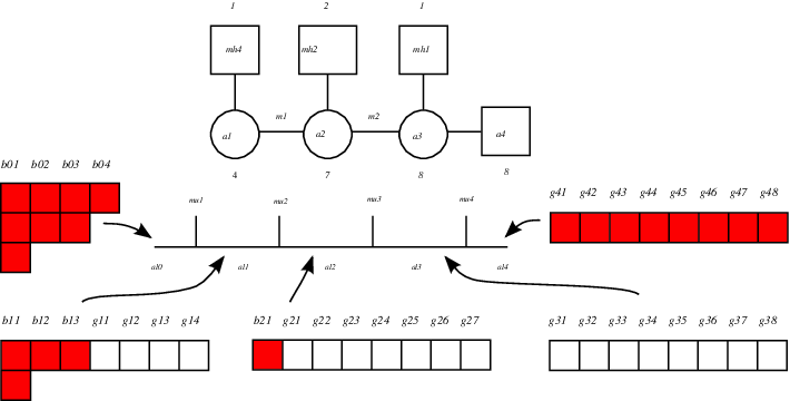
According to the AGT correspondence we should associate to each gauge theory a Riemann surface with punctures, decorated by mass parameters. In the case of linear quivers, the surface is a punctured sphere. The number of punctures is the number of gauge group components plus three.⁶⁶ 6 A simple way to do the counting it to recall that the complex moduli parameters of the surface are mapped to the gauge couplings.

Since the classification of quiver tails matches the physical semi-degenerate fields of Toda, it is natural to expect [8] that for each of the tails there will be one puncture with the semi-degenerate state. Indeed the analysis of the Seiberg-Witten curve for theories with a quiver tail gives a special singular point, and many other regular singularities (“simple punctures”). In the case of the theory in Figure 1 there are $k+1$ simple punctures, one full puncture, corresponding to the right-most matter in the quiver and a special puncture where we will insert the semi-degenerate state.

We expect to be able to reproduce the partition function of this gauge theory by studying Toda CFT on this Riemann surface. We consider the trivalent graph in Figure 2 representing the successive fusion of the semi-degenerate state $\alpha^{(0)}$ with simple-puncture states $\mu^{(l)}$. The intermediate states $\alpha^{(l)}$ with $1\leq l\leq k$ have to be integrated over. They should be related to the Coulomb branch parameters $a^{(l)}$, which take values in $i\mathbb{R}^{N_{l}-1}/S_{N_{l}}$, and therefore the states $\alpha^{(l)}$ should be restricted to such a subspace of primaries of Toda.

We can now state in a precise way the question we would like to answer:

1. 1.

   How are the mass parameters $m_{l}$ and $\hat{m}_{l}$ in the gauge theory encoded in the states $\mu^{(l)}$, $\alpha^{(0)}$ and $\alpha^{(k+1)}$.

2. 2.

   What are the allowed states $\alpha^{(l)}$ in the intermediate channels and how are they related to the Coulomb branch parameters $a^{(l)}$.

As a first test, though, we would like to check the consistency of the construction under decoupling of one of the gauge groups. We consider sending to zero the coupling of the first gauge multiplet, that of $SU(N_{1})$. In terms of the Riemann surface this is a degeneration limit where the neck connecting the first two punctures (with insertions $\alpha^{(0)}$ and $\mu^{(1)}$) is stretched to infinite length. In the limit this neck will look like a single puncture on the sphere with the state $\alpha^{(1)}$ and the same $k+1$ other operators as before.

On the gauge theory side we have the gauge group $SU(N_{2})\times\cdots\times SU(N_{k})$. The Coulomb branch parameters of $SU(N_{1})$ and $m_{1}$ are now frozen as mass parameters for $SU(N_{2})$. Looking at how we defined $\alpha^{(0)}$ and $\mu^{(1)}$ before exactly matches the definition of $\alpha^{(1)}$ and $\mu^{(2)}$ in terms of the new masses. The identification of all the other parameters $\alpha^{(l)}$ and $\mu^{(i+1)}$ for $i>1$ is not affected by the decoupling of the first $SU(N_{1})$, since their definitions depended only on parameters that appear in the quiver to the right of $SU(N_{2})$.

This can be done in more detail in the semiclassical approximation (ignoring $b$ and $b^{-1}$) by examining the Seiberg-Witten curve for these theories, which was written down in [13, 8]

where $c_{j}$ and $u^{(j)}_{s}$ with $s=2,\dots,N_{j}$ are the gauge coupling and a set of Coulomb branch parameters for the $j$-th gauge group. $\tilde{M}_{i}$ are the masses of the $N$ fundamental hypermultiplets coupling to the rightmost gauge group. $\hat{M}_{i}$ and $M_{i}$ are related to the masses of the fundamental hypermultiplets of the tail and the bifundamental matter.⁹⁹ 9 The physical masses of BPS states can be read from the poles in the Seiberg-Witten differential. The simplest (and most commonly cited) choice for the differential, which is $\lambda=v\,dz/z$, gives the correct physical masses only after a complicated linear transformation on the parameters $\hat{M}_{i}$ and $M_{i}$. This is explained for the case of $SU(2)$ with $N_{F}=4$ in [14] (see also the discussion in Appendix C of [15]). We perform this transformation in detail for the case of $SU(2)\times SU(3)$ in Section 3.4.

This curve was rewritten by Gaiotto in a different form [6]. First we collect all the terms with definite power of $v$

and then shift $v$ as $v\rightarrow v-\frac{M(z)}{N\Delta(z)}$. Considering the change of coordinate $v=xz$ the curve can be written as

In this way the Seiberg-Witten curve is written as an $N^{\text{th}}$ cover of a Reimann surface which in this case is the $k+3$ punctured sphere.

The functions $\Phi^{(I)}(z)$ have poles of order $I$ at the location of each of the punctures $z=z_{i}$ [6]

and it was shown in [1, 8] that in the semiclassical approximation the coefficient of the leading poles are the charges under the W-symmetry of the Toda state inserted at the puncture

It is straight-forward to read the parameters of the Toda states from the Seiberg-Witten curve, which is written explicitly in (2.14). One does has to take into account the shift in $v$ needed to write (2.16), which act by linear transformations on the mass parameters. Furthermore, as mentioned in footnote 9, these parameters are not exactly the physical masses in the theory. In Section 3.4 we do it in detail for the $SU(2)\times SU(3)$ theory. Here we study the allowed intermediate states in the general curve, but due to this difficulty, we discuss only the type of states, not the exact values of the mass parameters.

Looking at (2.14) and expanding around $z\sim 0$ we can identify in the semiclassical approximation [8]

where $\hat{M}_{i}^{(0)}=\hat{M}_{i}-\bar{M}^{(0)}$ and $\bar{M}^{(0)}=\frac{1}{N}\sum_{j=1}^{N_{1}}n_{j}\hat{M}_{j}$. Considering the parameterization (2.7), we have $\beta^{(0)}_{i}=\hat{M}_{i}^{(0)}$.

In order to analyze the internal state $\alpha^{(l)}$, we decouple the first $l$ gauge groups by setting $c_{j}=0$ for $j<l$. The Seiberg-Witten curve becomes

where $r_{i}$, with $i=1,\ldots,N_{l}$ are the roots of the polynomial

and thus satisfy $\sum_{i=1}^{N_{l}}r_{i}=M_{l}$. $r_{i}$ are the $N_{l}$ parameters of the Coulomb branch of the $SU(N_{l})$ gauge group. Defining $\hat{M}_{i}^{(l)}=\hat{M}_{i}-\bar{M}^{(l)}$ and $r_{i}^{(l)}=r_{i}-\bar{M}^{(l)}$ with

we can identify semiclassically

The analysis of the Seiberg-Witten curve thus confirm that the internal states $\alpha^{(l)}$ are of the form described in (2.9).

As mentioned above, the mass parameters as they appear in these states are not the physical masses, but are related to them by linear transformations. In fact, we can view our identification of states in Section 2.3 as filling in the information needed to complete the writing of the curve in Gaiotto form. The functions $\Phi^{(I)}(z)$ are completely determined by knowing their behavior near all their singularities. The leading poles give the W-charges of the external states. The lower order poles (like $\phi^{(I)}_{i,-1}$) satisfy certain constraints among them [8] which mirror the degeneracy conditions of the Toda states and after solving for these constraints, the remaining information parametrizes the Coulomb branch.

In the preceding section we proposed a map of the parameters between the quiver tails in ${\mathcal{N}}=2$ conformal gauge theories and correlation functions in Toda CFT with certain semi-degenerate states in the intermediate channels. The space of primary states in the intermediate channels is restricted by the conditions (2.11). Normally we should sum over all primary states in the intermediate channel. Our claim is that only the states we wrote down in (2.9) appear in the fusion rules of the other states (to the left) in the correlation function.

In the case of the $SU(2)\times SU(3)$ quiver, this claim amounts to saying that the fusion of two semi-degenerate states $\alpha^{(0)}$ and $\mu^{(1)}$ gives a state $\alpha^{(1)}$, which while not degenerate, does satisfy a condition restricting one of its two continuous parameters, $\beta^{(1)}$, to be related to $\beta^{(0)}$ and $\mu_{1}$ and in turn, to the masses in the gauge theory picture.

Being semi-degenerate means that the Verma module of the state $\alpha^{(0)}$, has a null states at level 1. This degeneracy condition allows to write a Ward identity on the three point function of $\alpha^{(0)}$, $\mu^{(1)}$ and $\alpha^{(1)}$. Due to the fact that $\mu^{(1)}$ is also semi-degenerate, this Ward identity can be written as a condition on the state $\alpha^{(1)}$. This Ward identity was written in [9] and we present here a slightly different derivation of it.

The degeneracy condition of $\alpha^{(0)}$ is given by

where

We would like to use the equation satisfied by $\alpha^{(0)}$ to derive a constraint on $\alpha^{(1)}$, so we need to commute the operators through $V_{\mu^{(1)}}(z)$. The action of $L_{n}$ and $W_{n}$ on the primaries is given by

By virtue of the degeneracy condition of the state $\mu$, which can be written as $[W_{-1},V_{\mu^{(1)}}]=\frac{3w_{\mu}}{2\Delta_{\mu}}[L_{-1},V_{\mu^{(1)}}]$, the combinations

have simple commutation relations with $V_{\mu^{(1)}}$

The degeneracy condition (3.2) can be written as

Permuting through $V_{\mu^{(1)}}(z)$ we get

Finally we can write the Ward identity by multiplying by ${\left|{\alpha^{(1)}}\right>}$ on the right. The degeneracy condition implies that this correlation function should vanish. Given that $\alpha^{(1)}$ is a primary, it is annihilated by $L_{1}$ and $W_{1}$ and satisfies $L_{0}|\alpha^{(1)}\rangle=\Delta_{1}|\alpha^{(1)}\rangle$ and $W_{0}|\alpha^{(1)}\rangle=w_{1}|\alpha^{(1)}\rangle$. We get an equation relating $w_{1}$ and $\Delta_{1}$ by

Therefore, for the three point function not to vanish, the prefactor has to. This is indeed the equation found by [9] which restricts the allowed primaries $\alpha^{(1)}$ in the intermediate channel of the $A_{2}$ description of $SU(2)\times SU(3)$ gauge theory.

To understand this equation it is useful to write the quantum numbers of the states as

Here $h_{i}$ are the weights of the fundamental representation, which for $SU(3)$ are

For the degenerate states parameterized in the orthonormal basis as in (3.1) we have

Plugging these relations into (3.9) we find the equation for the components of $\alpha^{(1)}$

The three different solutions to this equation are related, of course, by Weyl reflections. Using the parametrization of $\alpha^{(1)}$ in (3.1) we can choose the solution

As we see, though $\alpha^{(1)}$ is not a degenerate state, one of its components is fixed by the external parameters $\beta^{(0)}$ and $\mu_{1}$. The other parameter $\gamma^{(1)}_{1}=-\gamma^{(1)}_{2}$ is free, and should match the Coulomb branch parameter of the $SU(2)$ gauge group.

Within the AGT correspondence the product of the 1-loop determinants of the vector and hypermultiplets matches the three point functions associated to the fusion of successive primary states in the CFT.

In the following two sections we study the three point functions of semi-degenerate states in Toda CFT which are needed for the calculation of the quiver tail. In particular we show in Section 4 that imposing the condition (3.14) gives a pole in the three point function, whose residue is the desired three point function. In Section 5 we combine all the terms together and show in a more general setup that the 1-loop partition function agrees with the product of three point functions in Toda CFT. It is easy to plug in the states parameterized above in (3.1) into the resulting expressions, and we will not copy it here.

The upshot of that calculation is that it allows us to identify the gauge theory and Toda parameters as

Within the AGT correspondence, the instanton corrections to the gauge theory partition function [16, 17] match the contributions of descendants to the conformal blocks of the CFT. We turn now to analyzing this question for our case of the $SU(2)\times SU(3)$ gauge theory and its description within $A_{2}$ Toda CFT.

The relevant Toda correlator we are calculating is on the five-punctured sphere represented by the graphs in Figure 4. There are two intermediate states, $\alpha^{(1)}$ and $\alpha^{(2)}$ and the conformal blocks capture the contributions of all W-algebra descendants of these primaries

The expansion parameters $q^{(i)}$ are the complex structure moduli of the Riemann surface, related to the gauge groups couplings $\tau^{(i)}$ by $q^{(i)}=e^{2\pi i\tau^{(i)}}$. The sum is taken over all the descendants $|{\bf x};\alpha\rangle=L_{-x_{1}}\ldots L_{-x_{r}}W_{-\tilde{x}_{1}}\ldots W_{-\tilde{x}_{\tilde{r}}}|\alpha\rangle$, represented by the vectors ${\bf x}=(x_{1},\ldots,x_{r},\tilde{x}_{1},\ldots,\tilde{x}_{\tilde{r}})$ with $x_{1}\leq\dots\leq x_{r}$ and $\tilde{x}_{1}\leq\dots\leq\tilde{x}_{r}$. The level of the descendant is given by $|{\bf x}|=x_{1}+\ldots+x_{r}+\tilde{x}_{1}+\ldots+\tilde{x}_{\tilde{r}}$. $X^{-1}_{\bf x;\bf x^{\prime}}(\alpha)$ is the inverse of the Shapovalov matrix defined as $X_{\bf x;\bf x^{\prime}}(\alpha)=\langle\bf x;\alpha|\bf x^{\prime};\alpha\rangle$. The Shapovalov matrix is block diagonal, where any block correspond to a set of descendants with a given level. Restricting to a fixed level we define