跳到论文正文
W Papers独立论文阅读器 arXiv:1012.1271 论文正文 计算阅读时间 · 0%
引用这篇论文根据当前论文元数据生成,正式投稿前建议核对。


License: arXiv.org perpetual non-exclusive license
arXiv:1012.1271v1 [math.PR] 06 Dec 2010

Quasi-polynomial mixing of the 2d stochastic Ising model with “plus” boundary up to criticalityThanks: This work was supported by the European Research Council through the “Advanced Grant” PTRELSS 228032

Eyal Lubetzky Address: E. Lubetzky Microsoft Research One Microsoft Way Redmond, WA 98052-6399, USA. Email address: eyal@microsoft.com , Fabio Martinelli Address: F. Martinelli Dipartimento di Matematica Università Roma Tre Largo S. Murialdo 1 00146 Roma, Italia. Email address: martin@mat.uniroma3.it , Allan Sly Address: A. Sly Microsoft Research One Microsoft Way Redmond, WA 98052-6399, USA. Email address: allansly@microsoft.com and Fabio Lucio Toninelli Address: F.L. Toninelli CNRS and ENS Lyon Laboratoire de Physique 46 Allée d’Italie, 69364 Lyon, France. Email address: fabio-lucio.toninelli@ens-lyon.fr
Abstract.

We considerably improve upon the recent result of [33] on the mixing time of Glauber dynamics for the 2d Ising model in a box of side LL at low temperature and with random boundary conditions whose distribution 𝐏{\bf P} stochastically dominates the extremal plus phase. An important special case is when 𝐏{\bf P} is concentrated on the homogeneous all-plus configuration, where the mixing time TmixT_{\textsc{mix}} is conjectured to be polynomial in LL. In [33] it was shown that for a large enough inverse-temperature β\beta and any ε>0\varepsilon>0 there exists c=c⁡(β,ε)c=c(\beta,\varepsilon) such that limL→∞𝐏⁡(Tmix≥exp⁡(c​Lε))=0\lim_{L\to\infty}{\bf P}\left(T_{\textsc{mix}}\geq\exp({cL^{\varepsilon}})\right)=0. In particular, for the all-plus boundary conditions and β\beta large enough Tmix≤exp⁡(c​Lε)T_{\textsc{mix}}\leq\exp({cL^{\varepsilon}}).

Here we show that the same conclusions hold for all β\beta larger than the critical value βc\beta_{c} and with exp⁡(c​Lε)\exp({cL^{\varepsilon}}) replaced by Lc​log⁡LL^{c\log L} (i.e. quasi-polynomial mixing). The key point is a modification of the inductive scheme of [33] together with refined equilibrium estimates that hold up to criticality, obtained via duality and random-line representation tools for the Ising model. In particular, we establish new precise bounds on the law of Peierls contours which quantitatively sharpen the Brownian bridge picture established e.g. in [17, 19, 20].

Key words and phrases: 
Ising model, Mixing time, Phase coexistence, Glauber dynamics.
2010 Mathematics Subject Classification
60K35, 82C20

1. Introduction

The Ising model on lattices at and near criticality has been the focus of numerous research papers since its introduction in 1925, establishing it as one of the most studied models in mathematical physics. In two dimensions the model was exactly solved by Onsager [37] in 1944, determining its critical inverse-temperature βc=12​log⁡(1+2)\beta_{c}=\frac{1}{2}\log(1+\sqrt{2}) in the absence of an external magnetic field. While the classical study of the Ising model concentrated on its static properties, over the last three decades significant efforts were dedicated to the analysis of stochastic dynamical systems that both model its evolution and provide efficient methods of sampling it. Of particular interest is the interplay between the behaviors of the static and dynamical models as they both undergo a phase transition at the critical βc\beta_{c}.

The Glauber dynamics for the Ising model (also known as the stochastic Ising model), introduced by Glauber [16] in 1963, is considered to be the most natural sampling method for it, with notable examples including heat-bath and Metropolis. It is known that on a box of side-length LL in ℤ2\mathbb{Z}^{2} with free boundary conditions (b.c.), alongside the phase transition in the range of spin-spin correlations in the static Ising model around βc\beta_{c}, the corresponding Glauber dynamics exhibits a critical slowdown: Its mixing time (formally defined in §1.1) transitions from being logarithmic in LL in the high temperature regime β<βc\beta<\beta_{c} to being exponentially large in LL in the low temperature regime β>βc\beta>\beta_{c}, en route following a power law at the critical βc\beta_{c}.

One of the most fundamental open problems in the study of the stochastic Ising model is understanding the system’s behavior in the so-called phase-coexistence region under homogenous boundary conditions, e.g. all-plus boundary. In the presence of these b.c. the (−)(-) phase becomes unstable and as such the reduced bottleneck between the two phases drastically accelerates the rate of convergence of the dynamics to equilibrium. Indeed, in this case the Glauber dynamics is known to mix in time that is sub-exponential in the surface area of the box, contrary to its low-temperature behavior with free boundary. The central and longstanding conjecture addressing this phenomenon states that the mixing time of Glauber dynamics for the Ising model on a box of side-length LL with all-plus boundary conditions is at most polynomial in LL at any temperature.

So far this has been confirmed on the 2d lattice throughout the one-phase region β<βc\beta<\beta_{c} (see [28, 29]) and very recently at the critical β=βc\beta=\beta_{c} (see [27]). Despite intensive efforts over the last two decades, establishing a power-law behavior for the mixing of Glauber dynamics at the phase-coexistence region β>βc\beta>\beta_{c} under the all-plus b.c. remains an enticing open problem.

In [12] the precise order of mixing in this regime on a 2d square lattice of side-length LL was conjectured to be L2L^{2} in accordance with Lifshitz’s law (see [25] and also [9, 36, 44]). The heuristic behind this prediction argues that when a droplet of the (−)(-) phase is surrounded by the (+)(+) phase at low temperature it proceeds to shrink according to the mean-curvature of the interface between them. Unfortunately, rigorous analysis is still quite far from establishing the expected Lifshitz behavior of O⁡(L2)O(L^{2}) mixing.

Until recently the best upper bound on the mixing at the phase-coexistence region under the all-plus boundary was exp⁡(L1/2+o⁡(1))\exp(L^{1/2+o(1)}) due to [30] and valid for large enough β\beta. This bound from 1994 was substantially improved in a recent breakthrough paper [33], where it was shown (as a special case of a result on a wider class of b.c.) that for a sufficiently large β\beta and any ε>0\varepsilon>0 the mixing time is exp⁡(O⁡(Lε))\exp(O(L^{\varepsilon})). The approach of [33] hinged on a novel inductive scheme on boxes with random boundary conditions, combined with a careful use of the so-called Peres-Winkler censoring inequality; these ideas form the foundation of the present paper. Note that the requirement of large β\beta in [30, 33] was essential in order to make use of results of [11] on the Wulff construction, available only at low enough temperature by cluster expansion methods. For smaller values of β>βc\beta>\beta_{c} the best known estimates on the mixing time are due to [8] and of the weaker form exp⁡(o⁡(L))\exp(o(L)).

In this work we improve these estimates into an upper bound of the form LO⁡(log⁡L)L^{O(\log L)} on the mixing-time (i.e. quasi-polynomial in the side-length LL) valid for any β>βc\beta>\beta_{c}. The key to our analysis is a modification of the recursive framework introduced in [33] combined with refined equilibrium estimates that hold up to criticality. To establish these, in lieu of relying on cluster-expansions, we utilize duality and the random-line representation machinery for the high temperature Ising model developed in [40, 39].

A key new element of our proof concerns fine estimates on the fluctuations of cluster boundaries. Whenever the boundary is pinned at two vertices u=(0,0)u=(0,0) and v=(ℓ,0)v=(\ell,0), the contour of the cluster is known to converge to the Brownian bridge (cf. [10, 19, 20]). This does not, however, allow us to estimate the probability of events when these converge to 0 in the limit. In particular, we are interested in: (i) a Gaussian bound for the probability that the contour would reach height x​ℓx\sqrt{\ell} (established in Theorem 5.3); (ii) the probability that the contour remains in the upper half-plane, an event that would have probability 1/ℓ1/\ell were the contour to behave like a 1d random walk of length ℓ\ell conditioned to return to 0. In §5 (see Theorem 5.1) we prove that up to multiplicative constants this indeed holds for a given contour.

These then provide important tools in estimating the probability of various other events characterizing the Ising interfaces at equilibrium.

1.1. Glauber dynamics for the Ising model

Let Λ\Lambda be a generic finite subset of ℤ2{\mathbb{Z}}^{2}. Write x∼yx\sim y for the nearest-neighbor relation in ℤ2\mathbb{Z}^{2} (i.e. x∼yx\sim y if maxi=1,2⁡|xi−yi|=1\max_{i=1,2}|x_{i}-y_{i}|=1) and define ∂Λ\partial\Lambda, the boundary of Λ\Lambda, to be the nearest-neighbors of Λ\Lambda in ℤ2∖Λ\mathbb{Z}^{2}\setminus\Lambda:

∂Λ:={x∈ℤ2∖Λ:x∼y​ for some ​y∈Λ}.\partial\Lambda:=\{x\in\mathbb{Z}^{2}\setminus\Lambda\;:\;x\sim y\mbox{ for some }y\in\Lambda\}\,.

The classical Ising model on Λ\Lambda with no external magnetic field is a spin-system whose set of possible configurations is ΩΛ={−1,+1}Λ\Omega_{\Lambda}=\{-1,+1\}^{\Lambda}. Each configuration σ∈ΩΛ\sigma\in\Omega_{\Lambda} corresponds to an assignment of plus/minus spins to the sites in Λ\Lambda and has a statistical weight determined by the Hamiltonian

HΛτ(σ)=−∑x,y∈Λx∼yσxσy−∑x∈Λ,y∈∂Λx∼yσxτy,H_{\Lambda}^{\tau}(\sigma)=-\sum_{\begin{subarray}{c}x,y\in\Lambda\\ x\sim y\end{subarray}}\sigma_{x}\sigma_{y}-\sum_{\begin{subarray}{c}x\in\Lambda\,,\,y\in\partial\Lambda\\ x\sim y\end{subarray}}\sigma_{x}\tau_{y}\,,

where τ∈Ω∂Λ\tau\in\Omega_{\partial\Lambda} forms the boundary conditions (b.c.) of the system. The Gibbs measure associated to the spin-system with boundary conditions τ\tau is

πΛτ​(σ)=1Zβ,Λτ​e−β​HΛτ​(σ)(σ∈ΩΛ),\pi^{\tau}_{\Lambda}(\sigma)=\frac{1}{Z_{\beta,\Lambda}^{\tau}}e^{-\beta H_{\Lambda}^{\tau}(\sigma)}\qquad(\sigma\in\Omega_{\Lambda})\,, (1.1)

where β\beta is the inverse of the temperature (i.e. β=1T\beta=\frac{1}{T}) and the partition-function Zβ,ΛτZ_{\beta,\Lambda}^{\tau} is a normalizing constant. When the boundary conditions are uniformly equal to +1+1 (resp. −1-1) we will denote the Gibbs measure by πΛ+\pi_{\Lambda}^{+} (resp. πΛ−\pi_{\Lambda}^{-}). Throughout the paper we will omit the superscript τ\tau and the subscript Λ\Lambda from the notation of the Gibbs measure π\pi when these are made clear from the context.

The Gibbs measure enjoys a useful monotonicity property that will play a key role in our analysis. Consider the usual partial order on ΩΛ\Omega_{\Lambda} whereby σ≤η\sigma\leq\eta if σx≤ηx\sigma_{x}\leq\eta_{x} for all x∈Λx\in\Lambda. A function f:ΩΛ↦ℝf:\Omega_{\Lambda}\mapsto\mathbb{R} is monotone increasing (decreasing) if σ≤η\sigma\leq\eta implies f⁡(σ)≤f⁡(η)f(\sigma)\leq f(\eta) (f⁡(σ)≥f⁡(η)f(\sigma)\geq f(\eta)). An event is increasing (decreasing) if its characteristic function is increasing (decreasing). Given two probability measures μ,ν\mu,\nu on ΩΛ\Omega_{\Lambda} we say that μ\mu is stochastically dominated by ν\nu, denoted by μ⪯ν\mu\preceq\nu, if μ⁡(f)≤ν⁡(f)\mu(f)\leq\nu(f) for all increasing functions ff (here and in what follows μ⁡(f)\mu(f) stands for ∫f​𝑑μ\int fd\mu). According to these notations the well-known FKG inequalities [14] state that

  • •

    If τ≤τ′\tau\leq\tau^{\prime} then πΛτ⪯πΛτ′\pi_{\Lambda}^{\tau}\preceq\pi_{\Lambda}^{\tau^{\prime}}.

  • •

    If ff and gg are increasing then πΛτ​(f​g)≥πΛτ​(f)​πΛτ​(g)\pi_{\Lambda}^{\tau}(fg)\geq\pi_{\Lambda}^{\tau}(f)\pi_{\Lambda}^{\tau}(g).

The phase transition regime in the 2d Ising model occurs at low temperature and it is characterized by spontaneous magnetization in the thermodynamic limit. There is a critical value βc\beta_{c} such that for all β>βc\beta>\beta_{c},

limΛ→ℤ2πΛ+(σ0)=−limΛ→ℤ2πΛ−(σ0)=mβ>0.\lim_{\Lambda\to{\mathbb{Z}}^{2}}\pi_{\Lambda}^{+}(\sigma_{0})=-\lim_{\Lambda\to{\mathbb{Z}}^{2}}\pi_{\Lambda}^{-}(\sigma_{0})=m_{\beta}>0\,. (1.2)

Furthermore, in the thermodynamic limit the measures πΛ+\pi_{\Lambda}^{+} and πΛ−\pi_{\Lambda}^{-} converge (weakly) to two distinct Gibbs measures π∞+\pi^{+}_{\infty} and π∞−\pi^{-}_{\infty} which are measures on the space Ωℤ2\Omega_{\mathbb{Z}^{2}}, each representing a pure state. We will focus on this phase-coexistence region β>βc\beta>\beta_{c}.

The Glauber dynamics for the Ising model is a family of continuous-time Markov chains on the state space ΩΛ\Omega_{\Lambda}, reversible with respect to the Gibbs distribution πΛτ\pi_{\Lambda}^{\tau}. An important and natural example of this stochastic dynamics is the heat-bath dynamics, which we will now describe, postponing the formulation of the general Glauber dynamics to §2.1. Note that our results apply to all of these chains (e.g., Metropolis etc.) by standard arguments for comparing their mixing times (see e.g. [34]).

The heat-bath dynamics for the Ising model ΩΛ\Omega_{\Lambda} is defined as follows. With a rate one independent Poisson process for each vertex xx, the spin σx\sigma_{x} is refreshed by sampling a new value from the set {−1,+1}\{-1,+1\} according to the conditional Gibbs measure

πσ,xτ:=πΛτ(⋅∣σy,y≠x).\pi^{\tau}_{\sigma,x}:=\pi_{\Lambda}^{\tau}\left(\cdot\mid\sigma_{y},\,y\neq x\right)\,.

It is easy to verify that the heat-bath chain is indeed reversible with respect to πΛτ\pi_{\Lambda}^{\tau} and is characterized by the generator

(ℒΛτ​f)​(σ)=∑x∈Λ[πσ,xτ​(f)−f⁡(σ)],(\mathcal{L}_{\Lambda}^{\tau}f)(\sigma)=\sum_{x\in\Lambda}\left[\pi^{\tau}_{\sigma,x}(f)-f(\sigma)\right]\,,

where πσ,xτ​(f)\pi^{\tau}_{\sigma,x}(f) is the average of ff with respect to the conditional Gibbs measure πσ,xτ\pi^{\tau}_{\sigma,x} acting only on the variable σx\sigma_{x}. The Dirichlet form associated to ℒΛτ\mathcal{L}_{\Lambda}^{\tau} takes the form

ℰΛτ​(f,f)=∑x∈ΛπΛτ​(Varσ,xτ(f))\mathcal{E}_{\Lambda}^{\tau}(f,f)=\sum_{x\in\Lambda}\pi^{\tau}_{\Lambda}\left(\,\mathop{\rm Var}\nolimits^{\tau}_{\sigma,x}(f)\,\right)

where Varσ,xτ(f)\mathop{\rm Var}\nolimits^{\tau}_{\sigma,x}(f) denotes the variance with respect to πσ,xτ\pi^{\tau}_{\sigma,x}. It is possible to extend the above definition of the generator ℒΛτ\mathcal{L}_{\Lambda}^{\tau} directly to the whole lattice ℤ2{\mathbb{Z}}^{2} and get a well defined Markov process on Ωℤ2\Omega_{{\mathbb{Z}}^{2}} (see e.g. [26]). The latter will be referred to as the infinite volume Glauber dynamics, with generator denoted by ℒℤ2\mathcal{L}_{\mathbb{Z}^{2}}.

We will denote by μtσ\mu_{t}^{\sigma} the distribution of the chain at time tt when the starting configuration is identically equal to σ\sigma. For instance, for any ff and σ\sigma the expectation of ff w.r.t. μtσ\mu_{t}^{\sigma} is given by (TΛτ​(t))​f​(σ)(T_{\Lambda}^{\tau}(t))f(\sigma) where TΛτT_{\Lambda}^{\tau} is the Markov semigroup generated by ℒΛτ\mathcal{L}_{\Lambda}^{\tau}. The notation μt±\mu_{t}^{\pm} will stand for the corresponding quantity for an initial configuration of either all-plus or all-minus.

A key quantity that measures the rate of convergence of Glauber dynamics to stationarity is the gap in the spectrum of its generator, denoted by gapΛτ\text{\tt{gap}}_{\Lambda}^{\tau}. The Dirichlet form associated with ℒΛτ\mathcal{L}_{\Lambda}^{\tau} produces the following characterization for the spectral-gap:

gapΛτ=inffℰΛτ​(f,f)VarΛτ⁡(f),\text{\tt{gap}}_{\Lambda}^{\tau}=\inf_{f}\frac{\mathcal{E}_{\Lambda}^{\tau}(f,f)}{\operatorname{Var}^{\tau}_{\Lambda}(f)}\,,

where the infimum is over all nonconstant f∈L2​(πΛτ)f\in L^{2}(\pi_{\Lambda}^{\tau}). Another useful measure for the speed of relaxation to equilibrium is the total-variation mixing time which is defined as follows. Recall that the total-variation distance between two measures ϕ,ψ\phi,\psi on a finite probability space Ω\Omega is defined as

‖ϕ−ψ‖:=supA⊂Ω|ϕ⁡(A)−ψ⁡(A)|=12​∑x∈Ω|ϕ⁡(x)−ψ⁡(x)|.\|\phi-\psi\|:=\sup_{A\subset\Omega}\left|\phi(A)-\psi(A)\right|=\frac{1}{2}\sum_{x\in\Omega}|\phi(x)-\psi(x)|\,.

For any ε∈(0,1)\varepsilon\in(0,1), the ε\varepsilon-mixing-time of the Glauber dynamics is given by

Tmix​(ε):=inf{t>0:supσ∈ΩΛ‖μtσ−πΛτ‖≤ε}.T_{\textsc{mix}}(\varepsilon):=\inf\Bigl\{t>0:\sup_{\sigma\in\Omega_{\Lambda}}\|\mu_{t}^{\sigma}-\pi_{\Lambda}^{\tau}\|\leq\varepsilon\Bigr\}.

When ε=1/(2​e)\varepsilon=1/(2e) we will simply write TmixT_{\textsc{mix}}. This particular definition yields the following well-known inequalities (see e.g. [42, 24]):

supσ∈ΩΛ‖μtσ−πΛτ‖\displaystyle\sup_{\sigma\in\Omega_{\Lambda}}\|\mu_{t}^{\sigma}-\pi_{\Lambda}^{\tau}\| ≤exp(−⌊t/Tmix⌋) for all t≥0,\displaystyle\leq\exp(-\lfloor t/T_{\textsc{mix}}\rfloor)\quad\mbox{ for all $t\geq 0$}\,,
1gap≤Tmix\displaystyle\frac{1}{\text{\tt{gap}}}\leq T_{\textsc{mix}} ≤1gap​log⁡2​eπmin where ​πmin=minσ∈ΩΛ⁡πΛτ​(σ).\displaystyle\leq\frac{1}{\text{\tt{gap}}}\log\frac{2e}{\pi_{\min}}\qquad\mbox{ where }\pi_{\min}=\min_{\sigma\in\Omega_{\Lambda}}\pi_{\Lambda}^{\tau}(\sigma)\,.

The last inequality shows that in our setting gap−1\text{\tt{gap}}^{-1} and TmixT_{\textsc{mix}} are always within a factor of O⁡(|Λ|)O(|\Lambda|) from one another (to see this, observe that πΛτ​(σ)/πΛτ​(σ′)≤exp⁡(O⁡(|Λ|))\pi_{\Lambda}^{\tau}(\sigma)/\pi_{\Lambda}^{\tau}(\sigma^{\prime})\leq\exp(O(|\Lambda|)) for any σ,σ′∈ΩΛ\sigma,\sigma^{\prime}\in\Omega_{\Lambda} by Eq. (1.1) whereas |ΩΛ|=2|Λ||\Omega_{\Lambda}|=2^{|\Lambda|}). One could restate our results as well as the analogous conjecture on the polynomial mixing time under all-plus b.c. in terms of gap−1\text{\tt{gap}}^{-1} (expected to have order LL, the side-length of Λ\Lambda, for any β>βc\beta>\beta_{c}; see [5, 7]).

1.2. Main results

We are now in a position to formalize the main contribution of this paper. The following theorem is the counterpart of the main result obtained by two of the authors in [33]. Here we feature an improved estimate that in addition holds not only for large enough β\beta but throughout the phase-coexistence region.

Theorem 1.

For any β>βc\beta>\beta_{c} there exists some c⁡(β)>0c(\beta)>0 so that the following holds for the Glauber dynamics for the Ising model on the square ΛL\Lambda_{L} at inverse-temperature β\beta. If LL is of the form L=2n−1L=2^{n}-1 for some integer nn then:

  1. (1)

    If the boundary conditions τ\tau are sampled from a law 𝐏{\bf P} that either stochastically dominates the pure phase π∞+\pi^{+}_{\infty} or is stochastically dominated by π∞−\pi^{-}_{\infty} then

    𝐄​‖μtL±−πτ‖≤c/L for tL=Lc​log⁡L.\displaystyle{\bf E}\|\mu^{\pm}_{t_{L}}-\pi^{\tau}\|\leq c/L\quad\mbox{ for $t_{L}=L^{c\log L}$}\,. (1.3)

    In particular,

    𝐏⁡(Tmix≥Lc​log⁡L)≤c/L.\displaystyle{\bf P}\bigl(T_{\textsc{mix}}\geq L^{c\log L}\bigr)\leq c/L\,. (1.4)
  2. (2)

    The estimates (1.3),(1.4) also hold if 𝐏{\bf P} is stochastically dominated by π∞−\pi^{-}_{\infty} on one side of ΛL\Lambda_{L} and stochastically dominates π∞+\pi^{+}_{\infty} on the union of the other three sides. A similar statement holds if the roles of (+)(+) and (−)(-) are reversed.

The most natural consequence of the above result is obtained when 𝐏{\bf P} concentrates on homogenous boundary conditions, where the best previous bounds were exp⁡(O⁡(Lε))\exp(O(L^{\varepsilon})) for any ε>0\varepsilon>0 and β\beta large enough ([33]) along with exp⁡(o⁡(L))\exp(o(L)) for all other β>βc\beta>\beta_{c} ([8]).

Corollary 2.

For any β>βc\beta>\beta_{c} there exists some c⁡(β)>0c(\beta)>0 so that the mixing time of Glauber dynamics for the Ising model on the square ΛL\Lambda_{L} with b.c. τ≡+1\tau\equiv+1 satisfies

Tmix≤Lc​log⁡L.\displaystyle T_{\textsc{mix}}\leq L^{c\log L}\,. (1.5)

The same bound holds if the boundary conditions are (+)(+) on three sides and (−)(-) on the remaining one, and similarly if (+)(+) is replaced by (−)(-).

We believe that improving the above Lc​log⁡LL^{c\log L} bound into the conjectured polynomial one would require substantial new ideas. Indeed, in the present recursive framework in which the final scale of the system is reached via a doubling sequence, at each step the mixing-time estimate worsens by a power of LL (hence the quasi-polynomial bound). For a polynomial upper bound one could not afford to lose more than a constant factor on average along these steps.

One may also apply Theorem 1 to deduce the mixing behavior of the 2d Ising model under Bernoulli boundary conditions, as illustrated by the next corollary. Here and in what follows we say that an event holds with high probability (w.h.p.) to denote that its probability tends to 11 as the size of the system tends to ∞\infty.

Corollary 3.

Let β>βc\beta>\beta_{c} and consider Glauber dynamics for the Ising model on the square ΛL\Lambda_{L} with b.c. τ\tau comprised of i.i.d. Bernoulli variables, 𝐏⁡(τ⁡(x)=+1)=p+{\bf P}(\tau(x)=+1)=p_{+} for some p+≥12​(1+tanh⁡(4​β))p_{+}\geq\frac{1}{2}(1+\tanh(4\beta)). Then w.h.p. Tmix≤Lc​log⁡LT_{\textsc{mix}}\leq L^{c\log L} for some c⁡(β)>0c(\beta)>0.

To obtain the above corollary observe that the Bernoulli boundary conditions with the above specified p+p^{+} clearly stochastically dominate the marginal of π∞+\pi_{\infty}^{+} on ∂Λ\partial\Lambda.

The mixing time of Glauber dynamics for Ising on a finite box under all-plus b.c. is closely related to the asymptotic decay of the time auto-correlation function in the infinite-volume dynamics on ℤ2\mathbb{Z}^{2} started at the plus phase. Here it was conjectured in [12] that the decay should follow a stretched exponential of the form exp⁡(−c​t)\exp(-c\sqrt{t}). As a by-product of Corollary 2 (and standard monotonicity arguments) we obtain a new bound on this quantity, improving on the previous estimate due to [33] of exp⁡(−(log⁡t)c)\exp(-(\log t)^{c}) with arbitrarily large cc which was applicable for large enough β\beta.

Corollary 4.

Let β>βc\beta>\beta_{c}, let f⁡(σ)=σ0f(\sigma)=\sigma_{0} and define ρ⁡(t)≡Var∞+(et​ℒℤ2​f)\rho(t)\equiv\mathop{\rm Var}\nolimits^{+}_{\infty}\left(e^{t\mathcal{L}_{\mathbb{Z}^{2}}}f\right) to be the time autocorrelation of the spin at the origin started from the plus phase π∞+\pi^{+}_{\infty} (the variance is w.r.t. the plus phase π∞+\pi^{+}_{\infty}). Then there exists some c⁡(β)>0c(\beta)>0 such that for any tt,

ρ⁡(t)≤exp⁡(−ec​log⁡t).\rho(t)\leq\exp\bigl(-e^{c\sqrt{\log t}}\bigr)\,. (1.6)

1.3. Related work

Over the last two decades considerable effort was devoted to the formidable problem of establishing polynomial mixing for the stochastic Ising model on a finite lattice with all-plus b.c. Following is a partial account of related results.

Analogous to its conjectured behavior on ℤ2\mathbb{Z}^{2}, the mixing of Glauber dynamics for the Ising model on the lattice ℤd\mathbb{Z}^{d} in any fixed dimension dd is believed to be polynomial in the side-length of the box at any temperature in the presence of an all-plus boundary. Unfortunately, the state-of-the-art rigorous analysis of the problem in three dimensions and higher is far more limited. Faced with the polynomial lower bounds of [5], the best known upper bound for dimension d≥3d\geq 3 is exp⁡(Ld−2+o⁡(1))\exp(L^{d-2+o(1)}) for large enough β\beta (as usual LL being the side-length) due to [45]. Compare this with the case of no (i.e. free) boundary conditions case where it was shown in [46] that gap−1\text{\tt{gap}}^{-1} (and thus also TmixT_{\textsc{mix}}) is at least c​exp⁡(c′​β​Ld−1)c\exp(c^{\prime}\beta L^{d-1}) for some c=c⁡(β)>0c=c(\beta)>0 and an absolute constant c′>0c^{\prime}>0.

In two dimensions, ever since the work of Martinelli [30] in 1994 (an upper bound of exp⁡(L1/2+o⁡(1))\exp(L^{1/2+o(1)}) at low enough temperatures) and until quite recently no real progress has been made on the original problem. Nevertheless, various variants of this problem became fairly well understood. For instance, nearly homogenous boundary conditions were studied in [3, 2]. Analogues of the problem on non-amenable geometries (in terms of a suitable parameter measuring the growth of balls to replace the side-length) were established, pioneered by the work of [31] on trees and followed by results of [4] on a class of hyperbolic graphs of large degrees. The Solid-On-Solid model (SOS), proposed as an idealization of the behavior of Ising contours at low temperatures, was studied in [32] where the authors obtained several insights into the evolution of the contours. Finally, the conjectured Lifshitz behavior of O⁡(L2)O(L^{2}) was confirmed at zero temperature [9, 13, 7], with the recent work [7] providing sharp bounds also for near-zero temperatures (namely when β≥c​log⁡L\beta\geq c\log L for a suitably large c>0c>0) in both dimensions two and three.

As mentioned above, the exp⁡(L1/2)\exp(L^{1/2}) barrier was finally broken in the recent paper [33], replacing it by exp⁡(c​Lε)\exp(cL^{\varepsilon}) for an arbitrarily small ε>0\varepsilon>0 and sufficiently large β\beta (where the constant c=c⁡(β,ε)c=c(\beta,\varepsilon) diverges to +∞+\infty as ε→0\varepsilon\to 0). At the heart of the proof of the main result of that paper ([33]*Theorem 1.6) was an inductive procedure which will serve as our main benchmark here. We will shortly review that argument in §3 in order to motivate and better understand the new steps gained in the present work.

Finally, there is an extensive literature on the phase-separation lines in the 2d Ising model, going back to [1, 15]. In §2 we will review the tools we will need from the random-line representation framework of [40, 39]. For further information see e.g. [41] and the references therein.

2. Preliminaries

2.1. General Glauber dynamics

The class of Glauber dynamics for the Ising model on a finite box Λ⊂ℤ2\Lambda\subset\mathbb{Z}^{2} consists of the continuous-time Markov chains on the state space ΩΛ\Omega_{\Lambda} that are given by the generator

(ℒΛτ​f)​(σ)=∑x∈Λc⁡(x,σ)​(f⁡(σx)−f⁡(σ)),(\mathcal{L}^{\tau}_{\Lambda}f)(\sigma)=\sum_{x\in\Lambda}c(x,\sigma)\left(f(\sigma^{x})-f(\sigma)\right)\,, (2.1)

where σx\sigma^{x} is the configuration σ\sigma with the spin at xx flipped and the transition rates c⁡(x,σ)c(x,\sigma) should satisfy the following conditions:

  1. (1)

    Finite range interactions: For some fixed R>0R>0 and any x∈Λx\in\Lambda, if σ,σ′∈ΩΛ\sigma,\sigma^{\prime}\in\Omega_{\Lambda} agree on the ball of diameter RR about xx then c⁡(x,σ)=c⁡(x,σ′)c(x,\sigma)=c(x,\sigma^{\prime}).

  2. (2)

    Detailed balance: For all σ∈ΩΛ\sigma\in\Omega_{\Lambda} and x∈Λx\in\Lambda,

    c⁡(x,σ)c⁡(x,σx)=exp⁡(−β​∇xHΛτ​(σ)),\frac{c(x,\sigma)}{c(x,\sigma^{x})}=\exp\Bigl(-\beta\nabla_{x}H_{\Lambda}^{\tau}(\sigma)\Bigr)\,,

    where ∇xHΛτ​(σ)=HΛτ​(σx)−HΛτ​(σ)=2​σx​[∑y∈Λy∼xσy+∑y∈∂Λy∼xτy]\nabla_{x}H_{\Lambda}^{\tau}(\sigma)=H_{\Lambda}^{\tau}(\sigma^{x})-H_{\Lambda}^{\tau}(\sigma)=2\sigma_{x}\Bigl[\sum_{\begin{subarray}{c}y\in\Lambda\\ y\sim x\end{subarray}}\sigma_{y}+\sum_{\begin{subarray}{c}y\in\partial\Lambda\\ y\sim x\end{subarray}}\tau_{y}\Bigr].

  3. (3)

    Positivity and boundedness: The rates c⁡(x,σ)c(x,\sigma) are uniformly bounded from below and above by some fixed C1,C2>0C_{1},C_{2}>0.

  4. (4)

    Translation invariance: If σ≡σ′(⋅+ℓ)\sigma\equiv\sigma^{\prime}(\cdot+\ell), where ℓ∈Λ\ell\in\Lambda and addition is according to the lattice metric, then c⁡(x,σ)=c⁡(x+ℓ,σ′)c(x,\sigma)=c(x+\ell,\sigma^{\prime}) for all x∈Λx\in\Lambda.

The Glauber dynamics generator with such rates defines a unique Markov process, reversible with respect to the Gibbs measure μΛτ\mu_{\Lambda}^{\tau}. The two most notable examples for the choice of transition rates are

  1. (i)

    Metropolis: c⁡(x,σ)=exp⁡(−β​∇xHΛτ​(σ))∧ 1c(x,\sigma)=\exp\Bigl(-\beta\nabla_{x}H_{\Lambda}^{\tau}(\sigma)\Bigr)\;\wedge\;1\;.

  2. (ii)

    Heat-bath: c⁡(x,σ)=[1+exp⁡(β​∇xHΛτ​(σ))]−1\;c(x,\sigma)=\Bigl[1+\exp\bigl(\beta\nabla_{x}H_{\Lambda}^{\tau}(\sigma)\bigr)\Bigr]^{-1}\;.

See e.g. [34] for standard comparisons between these chains, in particular implying that their individual mixing times are within a factor of at most O⁡(|Λ|)O(|\Lambda|) from one another (hence our results apply to every one of these chains).

2.2. Surface tension

Denote by τβ​(θ)\tau_{\beta}(\theta) the surface tension that corresponds to the angle θ\theta, defined as follows. Associate with each angle θ∈[−π/4,π/4]\theta\in[-\pi/4,\pi/4] the unit vector n→θ=(cos⁡θ,sin⁡θ)∈𝕊1\vec{n}_{\theta}=(\cos\theta,\sin\theta)\in\mathbb{S}^{1} and the following b.c. ηθ\eta_{\theta} for ΛL={−⌊L/2⌋,…,⌊L/2⌋}2\Lambda_{L}=\{-\lfloor L/2\rfloor,\ldots,\lfloor L/2\rfloor\}^{2}:

ηθ​(v)={+1if ⟨v,n→θ⟩>0,−1if ⟨v,n→θ⟩≤0.\eta_{\theta}(v)=\left\{\begin{array}[]{ll}+1&\mbox{if $\left<v,\vec{n}_{\theta}\right>>0$}\,,\\ -1&\mbox{if $\left<v,\vec{n}_{\theta}\right>\leq 0$}\,.\end{array}\right.

Let Zβ,ΛLηθZ_{\beta,\Lambda_{L}}^{\eta_{\theta}} be the partition-function of the corresponding Ising model and, as usual, let Zβ,ΛL+Z_{\beta,\Lambda_{L}}^{+} denote the partition-function under the all-plus b.c. The surface tension in the direction orthogonal to n→θ\vec{n}_{\theta} is the limit

τβ(θ)=−limL→∞cos⁡θLlogZβ,ΛLηθZβ,ΛL+,\tau_{\beta}(\theta)=-\lim_{L\to\infty}\frac{\cos\theta}{L}\log\frac{Z_{\beta,\Lambda_{L}}^{\eta_{\theta}}}{Z_{\beta,\Lambda_{L}}^{+}}\,,

which gives rise to an even analytic function τβ\tau_{\beta} with period π/2\pi/2 on ℝ\mathbb{R} (a closed formula appears e.g. in [40]*Section 5). One can then extend the definition of τβ\tau_{\beta} to ℝ2\mathbb{R}^{2} by homogeneity, setting τβ​(x)=τβ​(θx)​|x|\tau_{\beta}(x)=\tau_{\beta}(\theta_{x})|x|, where |x||x| denotes the Euclidean norm of xx and θx\theta_{x} is the angle it forms with (1,0)(1,0). For all β>βc\beta>\beta_{c} this qualifies as a norm on ℝ2\mathbb{R}^{2}.

The surface tension measures the effect of the interface induced by the boundary conditions ηθ\eta_{\theta} on the free-energy and thus plays an important role in the geometry of the low temperature Ising model. For instance, it was shown in [43] that the large deviations of the magnetization in a square are governed by τβ​(0)\tau_{\beta}(0) (also see [22, 21]).

One of the useful properties of the surface tension is the sharp triangle inequality (see for instance [40]*Proposition 2.1): For any β>βc\beta>\beta_{c} there exists a strictly positive constant κβ\kappa_{\beta} such that for any x,y∈ℝ2x,y\in\mathbb{R}^{2} we have

τβ​(x)+τβ​(y)−τβ​(x+y)≥κβ​(|x|+|y|−|x+y|),\displaystyle\tau_{\beta}(x)+\tau_{\beta}(y)-\tau_{\beta}(x+y)\geq\kappa_{\beta}\left(|x|+|y|-|x+y|\right)\,, (2.2)

A thorough account of additional properties of the surface tension may be found e.g. in [11] and [41].

2.3. Duality

Let ℤ2∗:=ℤ2+(12,12){\mathbb{Z}}^{2*}:=\mathbb{Z}^{2}+(\frac{1}{2},\frac{1}{2}) denote the dual lattice to ℤ2{\mathbb{Z}}^{2}. The collection of edges of ℤ2{\mathbb{Z}}^{2} and of ℤ2∗{\mathbb{Z}}^{2*} will be denoted by Eℤ2E_{\mathbb{Z}^{2}} and Eℤ2∗∗E_{\mathbb{Z}^{2*}}^{*} respectively. It is useful to identify an edge e=(x,y)∈Eℤ2e=(x,y)\in E_{\mathbb{Z}^{2}} with the closed unit segment in ℝ2{\mathbb{R}}^{2} whose endpoints are {x,y}\{x,y\}, and similarly do so for edges in Eℤ2∗∗E_{\mathbb{Z}^{2*}}^{*}. To each edge e=(x,y)∈Eℤ2e=(x,y)\in E_{\mathbb{Z}^{2}} there corresponds a unique dual edge e∗∈Eℤ2∗∗e^{*}\in E_{\mathbb{Z}^{2*}}^{*} defined by the condition e∩e∗≠∅e\cap e^{*}\neq\emptyset.

Given a finite box Λ⊂ℤ2\Lambda\subset{\mathbb{Z}}^{2} of the form Λ={x=(x1,x2)∈ℤ2:|x1|≤L1,|x2|≤L2}\Lambda=\{x=(x_{1},x_{2})\in{\mathbb{Z}}^{2}:\ |x_{1}|\leq L_{1},\ |x_{2}|\leq L_{2}\}, the dual box Λ∗⊂ℤ2∗\Lambda^{*}\subset{\mathbb{Z}}^{2*} is Λ∗={x=(x1,x2)∈ℤ2∗:|x1|≤L1+12,|x2|≤L2+12}\Lambda^{*}=\{x=(x_{1},x_{2})\in{\mathbb{Z}}^{2*}:\ |x_{1}|\leq L_{1}+\frac{1}{2},\ |x_{2}|\leq L_{2}+\frac{1}{2}\}. The set of dual edges of Λ∗\Lambda^{*}, denoted by EΛ∗∗E^{*}_{\Lambda^{*}}, is the set of dual edges for which both endpoints lie in Λ∗\Lambda^{*}. Notice that for each edge e=(x,y)∈Eℤ2e=(x,y)\in E_{\mathbb{Z}^{2}} such that {x,y}∩Λ≠∅\{x,y\}\cap\Lambda\neq\emptyset, the corresponding dual edge e∗e^{*} necessarily belongs to EΛ∗∗E^{*}_{\Lambda^{*}}. These definitions readily generalize to an arbitrary finite 𝒢⊂ℤ2\mathcal{G}\subset{\mathbb{Z}}^{2}, in which case 𝒢∗⊂ℤ2∗\mathcal{G}^{*}\subset{\mathbb{Z}}^{2*} consists of all dual sites whose L1L^{1}-distance from 𝒢\mathcal{G} equals 11.

For any β>βc\beta>\beta_{c} we associate the dual inverse-temperature β∗\beta^{*} via the duality relation tanh⁡(β∗)=e−2​β\tanh(\beta^{*})=e^{-2\beta}. Notice that for any β>βc\beta>\beta_{c} the dual inverse temperature β∗\beta^{*} lies below βc\beta_{c} which is the unique fixed point of the map β↦β∗\beta\mapsto\beta^{*}. We will often refer to the Gibbs measure on a subset of the dual lattice Λ∗\Lambda^{*} at the inverse-temperature β∗\beta^{*} under free boundary, denoting it by πΛ∗∗\pi^{*}_{\Lambda^{*}}. The following well-known fact addresses the exponential decay of the two-point correlation function for the free Ising Gibbs measure above the critical temperature.

Lemma 2.1 (e.g. [35]*p309 Eq. (4.39), together with the GKS inequalities [18, 23]).

Let Λ⊂ℤ2\Lambda\subset\mathbb{Z}^{2} and β>βc\beta>\beta_{c}. There exists some Cβ>0C_{\beta}>0 such that for any x,y∈Λ∗x,y\in\Lambda^{*},

πΛ∗∗​(σx​σy)≤(Cβx−y∧1)​exp⁡(−τβ​(x−y)).\pi_{\Lambda^{*}}^{*}(\sigma_{x}\,\sigma_{y})\leq\left(\frac{C_{\beta}}{\sqrt{x-y}}\wedge 1\right)\exp\big(-\tau_{\beta}(x-y)\big)\,.

A matching exponent for the spin-spin correlation was established by [17] for two opposite points in the (dual) infinite strip. Let S={1,…,ℓ}×ℤS=\{1,\ldots,\ell\}\times\mathbb{Z} for some integer ℓ\ell and fix β>βc\beta>\beta_{c}. In the dual S∗S^{*} we let x=(12,12)x=(\frac{1}{2},\frac{1}{2}) and y=(ℓ+12,12)y=(\ell+\frac{1}{2},\frac{1}{2}) and consider the free Gibbs measure at inverse-temperature β∗\beta^{*}. It was shown in [17]*formula (2.22) that in this setting there exists some cβ>0c_{\beta}>0 such that

πS∗∗​(σx​σy)=cβ+o⁡(1)ℓ​exp⁡(−τβ​(0)​ℓ),\pi_{S^{*}}^{*}(\sigma_{x}\,\sigma_{y})=\frac{c_{\beta}+o(1)}{\sqrt{\ell}}\exp(-\tau_{\beta}(0)\ell)\,, (2.3)

where the o⁡(1)o(1)-term tends to 00 as ℓ→∞\ell\to\infty.

Figure 1. SE and SW splitting-rules for forming the contours

2.4. Contours

Let 𝒢=(V,E)\mathcal{G}=(V,E) be a finite subgraph of (ℤ2∗,Eℤ2∗∗)({\mathbb{Z}}^{2*},E_{\mathbb{Z}^{2*}}^{*}). The boundary of a subset of dual edges B⊂EB\subset E, denoted by δ​B\delta B, is the set of vertices of VV with an odd number of adjacent edges of BB. If δ​B=∅\delta B=\emptyset we say that BB is closed, otherwise it is open.

A chain of sites of length kk from xx to yy in 𝒢\mathcal{G} has the standard definition of a sequence of sites x=u0,u1,…,uk=yx=u_{0},u_{1},\ldots,u_{k}=y such that ui∈𝒢u_{i}\in\mathcal{G} and |ui−ui−1|=1|u_{i}-u_{i-1}|=1 for all ii. A ∗*-chain from xx to yy is similarly defined with the exception that the distance requirement is relaxed into 1≤|ui−ui−1|≤21\leq|u_{i}-u_{i-1}|\leq\sqrt{2} for all ii. A path from xx to yy in BB is a chain of sites consisting of edges of BB, that is (ui−1,ui)∈B(u_{i-1},u_{i})\in B for all ii. We say that a path is closed if its endpoint and starting point coincide, otherwise we say that it is open.

A set of dual edges B⊂EB\subset E can be uniquely partitioned into a finite number of edge-disjoint simple lines in E∩ℝ2E\cap{\mathbb{R}}^{2} called contours. This is achieved by repeating the following procedure referred to as the South-East (SE) splitting-rule: When four bonds meet at a vertex we separate them along the SE-oriented diagonal going through the intersection. Alternatively, one may globally apply the SW splitting-rule, analogously defined with the South-West orientation replacing the South-East one (see Figure 1).

Contours can be either open or closed (with the same distinction as in paths). The length of a contour γ\gamma, denoted by |γ||\gamma|, is the number of edges in γ\gamma, and the length of a collection of contours γ¯={γ1,…,γk}\underline{\gamma}=\{\gamma_{1},\ldots,\gamma_{k}\} will simply be the sum of all the individual lengths. Given a finite family of contours γ¯={γ1,…,γk}\underline{\gamma}=\{\gamma_{1},\ldots,\gamma_{k}\} we say that it is compatible if it is the contour decomposition of its collection of dual edges ∪iγi\cup_{i}\gamma_{i}. We further say that γ¯\underline{\gamma} is EE-compatible (or 𝒢\mathcal{G}-compatible) to emphasize that in addition all the edges of ∪iγi\cup_{i}\gamma_{i} belong to EE, the edge-set of 𝒢\mathcal{G}.

Given boundary conditions τ∈{−1,1}ℤ2\tau\in\{-1,1\}^{{\mathbb{Z}}^{2}} and a box Λ\Lambda, each spin-configuration σ\sigma compatible with τ\tau outside Λ\Lambda (i.e. σx=τx\sigma_{x}=\tau_{x} for any x∉Λx\notin\Lambda) can be uniquely specified by giving all the edges e=(x,y)∈Eℤ2e=(x,y)\in E_{\mathbb{Z}^{2}} such that σx≠σy\sigma_{x}\neq\sigma_{y} and {x,y}∩Λ≠∅\{x,y\}\cap\Lambda\neq\emptyset (that is, all edges whose endpoint sites disagree). Equivalently, one can specify the corresponding dual edges of Λ∗\Lambda^{*}. By applying the above contour decomposition we see that each configuration σ\sigma compatible with τ\tau is uniquely characterized by its collection of closed and open contours (see Figure 2 for an illustration). The open contours obtained in this manner are called the phase-separation lines.

Figure 2. Contour decomposition of the edge-set induced by an Ising configuration on a box with mixed boundary conditions according to both SE and SW splitting-rules.

It is clear that the boundary δ​λ¯\delta\underline{\lambda} of the open contours belongs to ∂Λ∗\partial\Lambda^{*} and must coincide with a certain set V⁡(τ)V(\tau) uniquely specified by the boundary conditions τ\tau (i.e. independent of the values σ\sigma gives to the spins of Λ\Lambda). Notice that the cardinality of V⁡(τ)V(\tau), if different from zero, must be even.

A family of closed and open simple lines γ¯\underline{\gamma} is called τ\tau-compatible if there exists a configuration σ\sigma compatible with τ\tau in Λ\Lambda from which γ¯\underline{\gamma} is obtained in the above procedure. One can easily verify that when Λ\Lambda is a box the set of τ\tau-compatible contours coincides with the set of EΛ∗∗E^{*}_{\Lambda^{*}}-compatible contours whose boundary is equal to V⁡(τ)V(\tau).

2.5. Random-line representation

For a finite subgraph 𝒢=(V,E)\mathcal{G}=(V,E) of (ℤ2∗,Eℤ2∗∗)({\mathbb{Z}}^{2*},E_{\mathbb{Z}^{2*}}^{*}) and an EE-compatible family of contours θ¯\underline{\theta}, two different partition functions Z⁡(𝒢)Z(\mathcal{G}) and Z⁡(𝒢|θ¯)Z(\mathcal{G}\thinspace|\thinspace\underline{\theta}) will turn out to be useful for a given β>0\beta>0:

Z⁡(𝒢)\displaystyle Z(\mathcal{G}) =∑γ¯:δ​γ¯=∅γ¯​ is E-compatiblee−2​β​|γ¯|,\displaystyle=\sum_{\begin{subarray}{c}\underline{\gamma}:\,\delta\underline{\gamma}=\emptyset\\ \underline{\gamma}\text{ is $E$-compatible}\end{subarray}}e^{-2\beta|\underline{\gamma}|}\,, (2.4)
Z⁡(𝒢|θ¯)\displaystyle Z(\mathcal{G}\thinspace|\thinspace\underline{\theta}) =∑γ¯:δ​γ¯=∅γ¯∪θ¯​ is E-compatiblee−2​β​|γ¯|.\displaystyle=\sum_{\begin{subarray}{c}\underline{\gamma}:\,\delta\underline{\gamma}=\emptyset\\ \underline{\gamma}\cup\underline{\theta}\text{ is $E$-compatible}\end{subarray}}e^{-2\beta|\underline{\gamma}|}\,. (2.5)

Using Z⁡(𝒢)Z(\mathcal{G}) and Z⁡(𝒢|θ¯)Z(\mathcal{G}\thinspace|\thinspace\underline{\theta}) we define the weight (not necessarily a probability distribution) corresponding to the family of contours θ¯\underline{\theta}, denoted by q𝒢​(θ¯)q_{\mathcal{G}}(\underline{\theta}), to be

q𝒢​(θ¯)={Z⁡(𝒢|θ¯)Z⁡(𝒢)​e−2​β​|θ¯|if θ¯ is E-compatible,0otherwise.q_{\mathcal{G}}(\underline{\theta})=\left\{\begin{array}[]{ll}\frac{Z(\mathcal{G}\thinspace|\thinspace\underline{\theta})}{Z(\mathcal{G})}\,e^{-2\beta|\underline{\theta}|}&\mbox{if $\underline{\theta}$ is $E$-compatible,}\\ 0&\mbox{otherwise.}\end{array}\right. (2.6)

The key reason for the above formula is the following random-line representation for even-point correlation functions: Consider the Ising model on 𝒢\mathcal{G} at inverse temperature β∗\beta^{*} and free boundary conditions. Let π𝒢∗\pi^{*}_{\mathcal{G}} be the associated Gibbs measure and let A⊂VA\subset V have even cardinality. Then the following holds (see [40]*Lemma 6.9):

∑λ¯:δ​λ¯=Aq𝒢(λ¯)=π𝒢∗(∏x∈Aσx).\sum_{\underline{\lambda}:\ \delta\underline{\lambda}=A}q_{\mathcal{G}}(\underline{\lambda})=\pi_{\mathcal{G}}^{*}\Big(\prod_{x\in A}\sigma_{x}\Big)\,. (2.7)
Remark.

If the cardinality of AA is odd then the r.h.s. of (2.7) is zero by symmetry and the l.h.s. is zero due to the definition of q𝒢​(λ¯)q_{\mathcal{G}}(\underline{\lambda}).

Back to the low temperature Ising model in a box Λ\Lambda with boundary condition τ\tau, let λ¯\underline{\lambda} be a collection of τ\tau-compatible open contours. Then, by construction,

πΛτ(σ:λ¯(σ)=λ¯)\displaystyle\pi^{\tau}_{\Lambda}\bigl(\sigma:\ \underline{\lambda}(\sigma)=\underline{\lambda}\bigr) =qΛ∗​(λ¯)∑λ¯′:δ​λ¯′=V⁡(τ)qΛ∗(λ¯′)=qΛ∗​(λ¯)πΛ∗∗(∏x∈V⁡(τ)σx),\displaystyle=\frac{q_{\Lambda^{*}}(\underline{\lambda})}{\sum_{\underline{\lambda}^{\prime}:\delta\underline{\lambda}^{\prime}=V(\tau)}q_{\Lambda^{*}}(\underline{\lambda}^{\prime})}=\frac{q_{\Lambda^{*}}(\underline{\lambda})}{\pi_{\Lambda^{*}}^{*}\bigr(\prod_{x\in V(\tau)}\sigma_{x}\bigl)}\,, (2.8)

where with a slight abuse of notation we have identified Λ∗\Lambda^{*} with the graph 𝒢=(Λ∗,EΛ∗∗)\mathcal{G}=(\Lambda^{*},E^{*}_{\Lambda^{*}}) and in the last equality we used (2.7). The above formula will be the starting point of the proof of the new equilibrium estimates, Propositions 4.4 and 4.5.

We conclude this section with some of the main properties of the weights q𝒢​(λ¯)q_{\mathcal{G}}(\underline{\lambda}). For further information see [40, 39].

Lemma 2.2 ([40]*Lemma 6.3).

Let 𝒢=(V,E)\mathcal{G}=(V,E) be a finite subgraph of (ℤ2∗,Eℤ2∗∗)({\mathbb{Z}}^{2*},E_{\mathbb{Z}^{2*}}^{*}) and let θ¯\underline{\theta} be a family of EE-compatible contours (open and closed). If 𝒢′\mathcal{G}^{\prime} is a subgraph of 𝒢\mathcal{G} then q𝒢′​(θ¯)≥q𝒢​(θ¯)q_{\mathcal{G}^{\prime}}(\underline{\theta})\geq q_{\mathcal{G}}(\underline{\theta}).

Remark.

Lemma 2.2 enables one to extend the definition of the weights q𝒢​(λ)q_{\mathcal{G}}(\lambda) for finite contours λ\lambda in a infinite graph 𝒢\mathcal{G} by taking a limit for n→∞n\to\infty of q𝒢n​(λ)q_{\mathcal{G}_{n}}(\lambda), where 𝒢n\mathcal{G}_{n} is the intersection of 𝒢\mathcal{G} with a box of size nn. By Lemma 2.2 the sequence q𝒢n​(λ)q_{\mathcal{G}_{n}}(\lambda) is monotone non-increasing and non-negative hence its limit indeed exists.

Let 𝒢=(V,E)\mathcal{G}=(V,E) be a subgraph of (ℤ2∗,Eℤ2∗∗)({\mathbb{Z}}^{2*},E_{\mathbb{Z}^{2*}}^{*}). The edge-boundary of an edge e∈Ee\in E, denoted by Δ⁡(e)\Delta(e), is comprised of the edge ee itself together with any edge e′∈Ee^{\prime}\in E that is incident to it and would belong to the same contour in the contour decomposition of EE via the agreed splitting-rule. For instance, with the SE splitting-rule the horizontal edge e=[(x,y),(x+1,y)]e=[(x,y),(x+1,y)] in the dual lattice ℤ2∗\mathbb{Z}^{2*} would have an edge-boundary of Δ⁡(e)={e,[(x,y),(x,y+1)],[(x+1,y),(x+1,y−1)]}\Delta(e)=\left\{e,[(x,y),(x,y+1)],[(x+1,y),(x+1,y-1)]\right\}. Given a subset of edges B⊂EB\subset E we define its edge-boundary as Δ(B)=∪e∈BΔ(e)\Delta(B)=\cup_{e\in B}\Delta(e). This definition implies that two contours λ\lambda and γ\gamma, where λ\lambda is closed and γ\gamma is either open or closed, are 𝒢\mathcal{G}-compatible if and only if the edge-set of λ\lambda does not intersect Δ⁡(γ)\Delta(\gamma) (see the related [40]*Lemma 6.1). The following lemma is a special case of [40]*Lemma 6.4):

Lemma 2.3 ([40]*Eq. (6.17)).

Let 𝒢=(V,E)\mathcal{G}=(V,E) be a subgraph of (ℤ2∗,Eℤ2∗∗)({\mathbb{Z}}^{2*},E_{\mathbb{Z}^{2*}}^{*}) and let θ¯\underline{\theta} and λ¯\underline{\lambda} denote two 𝒢\mathcal{G}-compatible families of contours with corresponding edge-sets Eθ¯E_{\underline{\theta}} and Eλ¯E_{\underline{\lambda}} respectively. If λ¯∪θ¯\underline{\lambda}\cup\underline{\theta} is 𝒢\mathcal{G}-compatible (or equivalently if Δ⁡(λ¯)∩Eθ¯=∅\Delta(\underline{\lambda})\cap E_{\underline{\theta}}=\emptyset) then

q𝒢​(θ¯∪λ¯)=q𝒢λ¯​(θ¯)​q𝒢​(λ¯),q_{\mathcal{G}}(\underline{\theta}\cup\underline{\lambda})=q_{\mathcal{G}_{\underline{\lambda}}}(\underline{\theta})q_{\mathcal{G}}(\underline{\lambda})\,,

where 𝒢λ¯\mathcal{G}_{\underline{\lambda}} is the subgraph of 𝒢\mathcal{G} given by the edge-set E∖Δ⁡(λ¯)E\setminus\Delta(\underline{\lambda}).

We will frequently need estimates on the weight of a contour constrained to go through certain dual sites; to this end, the following definition will be useful. Let 𝒢=(V,E)\mathcal{G}=(V,E) and let λ1,λ2\lambda_{1},\lambda_{2} be two open contours such that δ​λ1={x,y}\delta\lambda_{1}=\{x,y\} and δ​λ2={u,v}\delta\lambda_{2}=\{u,v\}. We say that λ1,λ2\lambda_{1},\lambda_{2} are disjoint if either they are 𝒢\mathcal{G}-compatible or their edge-sets are disjoint and the contour decomposition of the union of their edges is a single contour λ\lambda. Observe that in the latter case necessarily {x,y}∩{u,v}≠∅\{x,y\}\cap\{u,v\}\neq\emptyset. For a pair of disjoint open contours λ1,λ2\lambda_{1},\lambda_{2} we write λ1⊔λ2\lambda_{1}\sqcup\lambda_{2} to denote either the collection (λ1,λ2)(\lambda_{1},\lambda_{2}) in the former case or the single contour λ\lambda in the latter.

Lemma 2.4 ([40]*Lemma 6.5).

Let 𝒢=(V,E)\mathcal{G}=(V,E) be a graph in the dual lattice ℤ2∗\mathbb{Z}^{2*}. For any x,y,u,v∈Vx,y,u,v\in V,

∑λ¯=λ1⊔λ2δ​λ1={x,y},δ​λ2={u,v}q𝒢​(λ¯)≤∑λ1δ​λ1={x,y}q𝒢​(λ1)​∑λ2δ​λ2={u,v}q𝒢​(λ2).\sum_{\begin{subarray}{c}\underline{\lambda}=\lambda_{1}\sqcup\lambda_{2}\\ \delta\lambda_{1}=\{x,y\}\,,\,\delta\lambda_{2}=\{u,v\}\end{subarray}}q_{\mathcal{G}}(\underline{\lambda})\leq\sum_{\begin{subarray}{c}\lambda_{1}\\ \delta\lambda_{1}=\{x,y\}\end{subarray}}q_{\mathcal{G}}(\lambda_{1})\sum_{\begin{subarray}{c}\lambda_{2}\\ \delta\lambda_{2}=\{u,v\}\end{subarray}}q_{\mathcal{G}}(\lambda_{2})\,.

In particular,

Corollary 2.5 ([39]*Eq. (5.29)).

Let 𝒢=(V,E)\mathcal{G}=(V,E) be a graph in the dual lattice ℤ2∗\mathbb{Z}^{2*}. For any β>βc\beta>\beta_{c} and any u,v,z∈Vu,v,z\in V,

∑λ:δ​λ={u,v}z∈λq𝒢(λ)\displaystyle\sum_{\begin{subarray}{c}\lambda:\,\delta\lambda=\{u,v\}\\ z\in\lambda\end{subarray}}q_{\mathcal{G}}(\lambda) ≤(∑λ:δ​λ={u,z}q𝒢(λ))(∑λ:δ​λ={z,v}q𝒢(λ))=π𝒢∗(σuσz)π𝒢∗(σvσz).\displaystyle\leq\biggl(\sum_{\lambda:\,\delta\lambda=\{u,z\}}q_{\mathcal{G}}(\lambda)\biggr)\biggl(\sum_{\lambda:\,\delta\lambda=\{z,v\}}q_{\mathcal{G}}(\lambda)\biggr)=\pi_{\mathcal{G}}^{*}\left(\sigma_{u}\,\sigma_{z}\right)\,\pi_{\mathcal{G}}^{*}\left(\sigma_{v}\,\sigma_{z}\right)\,.

Together with Lemma 2.1 the above lemma immediately implies an upper bound on the weights in mention in terms of the surface tensions τβ​(u−v)\tau_{\beta}(u-v) and OPENτβ​(v−z))\tau_{\beta}(v-z)). The next lemma provides an analogous bound for the weights of closed contours going through a set of prescribed sites.

Lemma 2.6 ([39]*Lemma 5.5 part (ii)).

Let 𝒢=(V,E)\mathcal{G}=(V,E) be a graph in ℤ2∗\mathbb{Z}^{2*}. Let x1,…,xk∈Vx_{1},\ldots,x_{k}\in V and identify x0≡xkx_{0}\equiv x_{k}. Then

∑λ:δ​λ=∅x1,…,xk∈λq𝒢(λ)≤exp(−∑i=1kτβ(xi−xi−1)).\sum_{\begin{subarray}{c}\lambda:\delta\lambda=\emptyset\\ x_{1},\ldots,x_{k}\in\lambda\end{subarray}}q_{\mathcal{G}}(\lambda)\leq\exp\bigg(-\sum_{i=1}^{k}\tau_{\beta}(x_{i}-x_{i-1})\bigg)\,.

3. Inductive framework for rectangles with “plus” boundaries

In this section we outline the recursive scheme developed in [33] which, as mentioned in §1, established a significantly improved upper bound of exp⁡(c​Lε)\exp(cL^{\varepsilon}) for the mixing time on a box of side-length LL with “plus” b.c. at sufficiently low temperatures.

Given ε>0\varepsilon>0 (to be thought of as very small) and L∈ℕL\in\mathbb{N} let

RL={x=(i,j)∈ℤ2: 1≤i≤L, 1≤j≤⌈L12+ε⌉}.R_{L}=\{x=(i,j)\in{\mathbb{Z}}^{2}:\ 1\leq i\leq L,\,1\leq j\leq\lceil L^{\frac{1}{2}+\varepsilon}\rceil\}.

Similarly one defines the rectangle QLQ_{L}, the only difference being that the vertical sides contain now ⌈(2​L+1)12+ε⌉\lceil(2L+1)^{\frac{1}{2}+\varepsilon}\rceil sites.

Definition 3.1.

A distribution 𝐏{\bf P} of b.c. for a rectangle RR (which will be RLR_{L}, QLQ_{L} or some translation of them) is said to belong to 𝒟⁡(R)\mathcal{D}(R) if its marginal on the union of North, East and West borders of RR is stochastically dominated by (the marginal of) the minus phase π∞−\pi^{-}_{\infty} of the infinite system, while the marginal on the South border of RR dominates the (marginal of the) infinite plus phase π∞+\pi^{+}_{\infty}.

The most natural example is to take 𝐏{\bf P} concentrated on the boundary condition τ≡−1\tau\equiv-1 on the North, East and West borders, and τ≡+1\tau\equiv+1 on the South border.

Definition 3.2.

For any given L∈ℕ,δ>0,t>0L\in\mathbb{N},\delta>0,t>0 consider the Ising model in RLR_{L}, with boundary condition τ\tau chosen from some distribution 𝐏\bf P. We say that 𝒜⁡(L,t,δ)\mathcal{A}(L,t,\delta) holds if

𝐄​‖μt±−πτ‖≤δ\displaystyle{\bf E}\|\mu^{\pm}_{t}-\pi^{\tau}\|\leq\delta (3.1)

for every 𝐏∈𝒟⁡(RL){\bf P}\in\mathcal{D}(R_{L}). The statement ℬ⁡(L,t,δ)\mathcal{B}(L,t,\delta) is defined similarly, the only difference being that the rectangle RLR_{L} is replaced by QLQ_{L} (and 𝐏{\bf P} is required to belong to 𝒟⁡(QL)\mathcal{D}(Q_{L})).

With these definitions the iterative scheme developed in [33] can be summarized as follows.

Proposition 3.3 (The starting point).

For every β\beta (thus not necessarily large) there exists c=c⁡(β)c=c(\beta) such that for every L∈ℕL\in\mathbb{N} the statements 𝒜⁡(L,t,e−t​e−c​L1/2+ε)\mathcal{A}(L,t,e^{-t\,e^{-cL^{1/2+\varepsilon}}}) and ℬ⁡(L,t,e−t​e−c​L1/2+ε)\mathcal{B}(L,t,e^{-t\,e^{-cL^{1/2+\varepsilon}}}) hold.

Remark.

Notice that the factor e−c​L1/2+εe^{-cL^{1/2+\varepsilon}} in front of the time tt is nothing but the negative exponential of the shortest side of the rectangle.

Theorem 3.4 (The inductive step).

For every β\beta large enough there exist constants c1,c2,c3c_{1},c_{2},c_{3} such that:

𝒜⁡(L,t,δ)⇒ℬ⁡(L,t1,δ1)⇒𝒜⁡(2​L+1,t2,δ2)\mathcal{A}(L,t,\delta)\Rightarrow\mathcal{B}(L,t_{1},\delta_{1})\Rightarrow\mathcal{A}(2L+1,t_{2},\delta_{2}) (3.2)

where

δ1\displaystyle\delta_{1} =c1​(δ+e−c2​L2​ε+L2​e−c2​log⁡t)\displaystyle=c_{1}\left(\delta+e^{-c_{2}L^{2\varepsilon}}+L^{2}e^{-c_{2}\log t}\right) ; t1\displaystyle t_{1} =2​t\displaystyle=2t (3.3)
δ2\displaystyle\delta_{2} =c1​(δ1+e−c2​L3​ε)=c3​(δ+e−c2​L2​ε+L2​e−c2​log⁡t)\displaystyle=c_{1}(\delta_{1}+e^{-c_{2}L^{3\varepsilon}})=c_{3}(\delta+e^{-c_{2}L^{2\varepsilon}}+L^{2}e^{-c_{2}\log t}) ; t2\displaystyle t_{2} =ec3​L3​ε​t1=2​ec3​L3​ε​t\displaystyle=e^{c_{3}L^{3\varepsilon}}t_{1}=2e^{c_{3}L^{3\varepsilon}}t (3.4)
Remark.

In the original statement in [33] the obvious requirement of β\beta large was missing due to a typo.

Corollary 3.5 (Solving the recursion).

In the same setting of Theorem 3.4, for every L∈{2n−1}n∈ℕL\in\{2^{n}-1\}_{n\in\mathbb{N}} there exists

Δ⁡(L)≤exp⁡(−c′​Lε2)\displaystyle\Delta(L)\leq\exp\left(-c^{\prime}L^{\varepsilon^{2}}\right) (3.5)

such that 𝒜⁡(L,t,Δ⁡(L))\mathcal{A}\left(L,t,\Delta(L)\right) holds for every t≥T⁡(L):=ec​L3​εt\geq T(L):=e^{cL^{3\varepsilon}}.

In turn, at the basis of the proof of Theorem 3.4, besides the so called Peres-Winkler censoring inequality (see [38] and [33]*Section 2.4), there were two key equilibrium estimates on the behavior of (very) low temperature Ising interfaces which we now recall and which were the responsible for both the various e−Lεe^{-L^{\varepsilon}} error terms in δ1,δ2\delta_{1},\delta_{2} and the constraint β≫1\beta\gg 1 on the inverse-temperature. The latter was necessary since the techniques of [33] were based on several results of [11] on the Wulff construction which in turn use in an essential way low temperature cluster expansion.

3.1. Equilibrium bounds on low temperature Ising interfaces used in [33]

The first estimate is the key for the proof of the first part of the inductive statement namely 𝒜⁡(L,t,δ)⇒ℬ⁡(L,t1,δ1)\mathcal{A}(L,t,\delta)\Rightarrow\mathcal{B}(L,t_{1},\delta_{1}). Given the rectangle QLQ_{L} write it as the union of two overlapping rectangles, each of which is a suitable vertical translate of the rectangle RLR_{L} (see Figure 3).

Refer to caption
Figure 3. The box QLQ_{L} and its covering with the rectangles A,BA,B.

Call BB the lowest rectangle and AA the highest one. Then

Lemma 3.6 (see Claim 3.6 in [33]).

There exists c=c⁡(β,ε)>0c=c(\beta,\varepsilon)>0 such that

∑x∈Bc𝐄(πτ(σx=+)−πτ,−(σx=+))≤e−c​L2​ε\displaystyle\sum_{x\in B^{c}}{\bf E}\left(\pi^{\tau}(\sigma_{x}=+)-\pi^{\tau,-}(\sigma_{x}=+)\right)\leq e^{-cL^{2\varepsilon}} (3.6)

where πτ,−\pi^{\tau,-} denotes the Gibbs measure in QLQ_{L} with minus boundary conditions on its lowest side and τ\tau on the other three sides.

In turn, by suitably playing with monotonicity properties of the measure π\pi as a function of the boundary conditions (see the short discussion in the proof of Claim 3.6 in [33]), the proof of the Lemma can be reduced to establishing the following bound.

Consider the enlarged rectangle ELE_{L} with sides 3​L3L and 2​⌈(2​L+1)12+ε⌉2\lceil(2L+1)^{\frac{1}{2}+\varepsilon}\rceil respectively, which can be viewed as consisting of six rectangles QLQ_{L} stacked together. Let π(−,−,+,−)\pi^{(-,-,+,-)} be the associated Gibbs measure with (−)(-) boundary conditions on the North, East and West sides and (+)(+) on the South side. For any spin configuration σ∈{−1,+1}EL\sigma\in\{-1,+1\}^{E_{L}} let γ=γ⁡(σ)\gamma=\gamma(\sigma) denote the unique open contour corresponding to these boundary conditions. Then

Lemma 3.7.

For any β\beta large enough there exists c=c⁡(β,ε)c=c(\beta,\varepsilon) such that for any LL

π(−,−,+,−)​(γ​ reaches height ​L12+ε)≤e−c​L2​ε\pi^{(-,-,+,-)}\Bigl(\gamma\text{ reaches height }L^{\frac{1}{2}+\varepsilon}\Bigr)\leq e^{-cL^{2\varepsilon}} (3.7)

Notice that the height L12+εL^{\frac{1}{2}+\varepsilon} is well beyond the typical O⁡(L)O(\sqrt{L}) fluctuations of the interface.

The second equilibrium bound is required for the proof of the statement ℬ⁡(L,t1,δ1)⇒𝒜⁡(2​L+1,t2,δ2)\mathcal{B}(L,t_{1},\delta_{1})\Rightarrow\mathcal{A}(2L+1,t_{2},\delta_{2}) (see Section 3.2 and in particular Claim 3.10 in [33]). Here the bottom line is the following bound.

Let R¯L\bar{R}_{L} consists of two copies of RLR_{L} stacked one on top of the other. Let Δ⊂∂R¯L\Delta\subset\partial\bar{R}_{L} consists of those boundary sites x=(i,j)x=(i,j) in the South border such that |i−L/2|≤12​L3​ε|i-L/2|\leq\frac{1}{2}L^{3\varepsilon} and j=0j=0. Consider the Gibbs measure πR¯L(−,+,Δ)\pi_{\bar{R}_{L}}^{(-,+,\Delta)} on R¯L\bar{R}_{L} with (−)(-) boundary conditions on the union of the North boundary and Δ\Delta and (+)(+) on the rest of ∂R¯L\partial\bar{R}_{L}. Let Γ1\Gamma_{1} be the event that the open contour γ1\gamma_{1} starting on the upper left corner of R¯L\bar{R}_{L} ends at the left end of the interval Δ\Delta without ever crossing the vertical line at i=L/2i=L/2. Then

Lemma 3.8.

For any β\beta large enough there exists c=c⁡(β,ε)c=c(\beta,\varepsilon) such that for any LL

πR¯L(−,+,Δ)​(Γ1c)≤e−c​L3​ε\pi_{\bar{R}_{L}}^{(-,+,\Delta)}\bigl(\Gamma^{c}_{1}\bigr)\leq e^{-cL^{3\varepsilon}} (3.8)

In the scheme envisaged in [33] the role played by the tiny extra piece of (+)(+) boundary conditions at the vertices of Δ\Delta, being the main source of the ec3​L3​εe^{c_{3}L^{3\varepsilon}} factor relating the time scales t2,t1t_{2},t_{1} in (3.3), is quite crucial and therefore it needs a bit of explanation.

Figure 4. Two possible arrangements for the open Peierls contours in the Gibbs measure under a (−,+,Δ)(-,+,\Delta) boundary condition.

Let us first explain why the length of Δ\Delta was chosen equal to L3​εL^{3\varepsilon}. Under the boundary conditions (−,+,Δ)(-,+,\Delta), for any configuration there exist exactly two open Peierls contours γ1,γ2\gamma_{1},\gamma_{2} with two possible scenarios for their endpoints (illustrated in Figure 4):

  1. (a)

    γ1\gamma_{1} joins the two upper corners of R¯L\bar{R}_{L} and γ2\gamma_{2} the two ends of the interval Δ\Delta;

  2. (b)

    γ1\gamma_{1} joins the left upper corner of R¯L\bar{R}_{L} with the left boundary of Δ\Delta whereas γ2\gamma_{2} joins the right upper corner of R¯L\bar{R}_{L} with the right boundary of Δ\Delta.

In [33] it was shown, using a significant part of the main machinery of [11], that the ratio between the probabilities of the two cases is roughly of the form e−β⁡(L+|Δ|−2​D)​τβ​(0)e^{-\beta(L+|\Delta|-2D)\tau_{\beta}(0)} where DD is the Euclidean distance between the left upper corner of R¯L\bar{R}_{L} and the left boundary of Δ\Delta. Clearly D≈L/2−|Δ|+O⁡(L2​ε)D\approx L/2-|\Delta|+O(L^{2\varepsilon}) and therefore case (b) is much more likely than case (a) iff |Δ|≫L2​ε|\Delta|\gg L^{2\varepsilon}. The choice L3​εL^{3\varepsilon} was clearly not optimal and just a very safe one. Once the first scenario can be neglected then the fact that γ1\gamma_{1} does not intersect the vertical line at i=L/2i=L/2 is quite natural (but painful to prove).

Next we sketchily explain why the need of attracting the contour γ1\gamma_{1} deep down inside the rectangle R¯L\bar{R}_{L}.

When proving the implication ℬ⁡(L,t1,δ1)⇒𝒜⁡(2​L+1,t2,δ2)\mathcal{B}(L,t_{1},\delta_{1})\Rightarrow\mathcal{A}(2L+1,t_{2},\delta_{2}) we can imagine that the rectangle R2​L+1R_{2L+1} is written as the union of three copies of the rectangle QLQ_{L} denoted by QLcentr,QLleft,QLrightQ_{L}^{\text{centr}},Q_{L}^{\text{left}},Q_{L}^{\text{right}} (see Figure 5).

Refer to caption
Figure 5. The box R2​L+1R_{2L+1} and its covering with QLcentr,QLleft,QLrightQ_{L}^{\text{centr}},Q_{L}^{\text{left}},Q_{L}^{\text{right}}. In bold the exceptional set Δ\Delta.

For simplicity suppose that the boundary conditions around R2​L+1R_{2L+1} are the “extreme ones” namely (−,−,+,−)(-,-,+,-) ordered clockwise starting from the North one and imagine starting the dynamics from all pluses.

The Peres-Winkler results allow us to e.g. first run the dynamics in the central rectangle QLcentrQ_{L}^{\text{centr}} for a time t1t_{1} and then in the left and right ones for some other time lag. Thus the dynamics in QLcentrQ_{L}^{\text{centr}} runs with b.c. (−,+,+,+)(-,+,+,+) and after a time lag t1t_{1} it will be close to the Gibbs measure πQLcentr(−,+,+,+)\pi^{(-,+,+,+)}_{Q_{L}^{\text{centr}}} by less than δ1\delta_{1} because of ℬ⁡(L,t1,δ1)\mathcal{B}(L,t_{1},\delta_{1}). The trouble is that the marginal of this measure on e.g. the East boundary of QLleftQ_{L}^{\text{left}} is not dominated by π∞−\pi_{\infty}^{-} because the unique open contour joining the left upper corner of QLcentrQ_{L}^{\text{centr}} to the right one will stay close to the upper side of QLcentrQ_{L}^{\text{centr}}. Therefore we cannot use statement ℬ⁡(L,t1,δ1)\mathcal{B}(L,t_{1},\delta_{1}) for the dynamics in QLleftQ_{L}^{\text{left}} to force equilibrium there in another time lag t1t_{1}.

An appealing and very intuitive possible way out of this serious problem would be to run many times the dynamics in QLcentrQ_{L}^{\text{centr}} until a large deviation forces the open contour to go below and to the left of the East side of QLleftQ_{L}^{\text{left}}. Since the probability of this fluctuation is O⁡(exp⁡(−c​L2​ε))O(\exp(-cL^{2\varepsilon})) it would be enough to wait O⁡(exp⁡(c​L2​ε)​t1)O(\exp(cL^{2\varepsilon})t_{1}) runs. However a rigorous implementation of this idea is far from trivial and in [33] the solution was another one, less natural but much easier to carry out.

If one, by brute force, flips the boundary conditions inside the interval Δ\Delta on the South side of QLcentrQ_{L}^{\text{centr}} to (−)(-) the mixing time of the dynamics cannot change by more that exp⁡(c⁡(β)​|Δ|)\exp(c(\beta)|\Delta|) (see [33]*Section 2.5 for more details). Once the boundary conditions have been flipped then, thanks to (3.8), the contours in QLcentrQ_{L}^{\text{centr}} will follow scenario (b) above and the resulting distribution over the East boundary of QLleftQ_{L}^{\text{left}} will now be dominated by the minus phase π∞−\pi_{\infty}^{-} allowing another application of the inductive statement ℬ⁡(L,t1,δ1)\mathcal{B}(L,t_{1},\delta_{1}) to QLleftQ_{L}^{\text{left}} and QLrightQ_{L}^{\text{right}}.

4. A new recursive scheme

In this section we modify the recursion scheme of [33] and, modulo two equilibrium estimates very similar to Lemma 3.7 and 3.8, we prove Theorem 1. We begin by fixing some notation.

Let N∈ℕN\in\mathbb{N} be a large integer, let L=LN=2N−1L=L_{N}=2^{N}-1 and choose N0N_{0} to be the smallest integer such that LN0:=2N0−1≥⌊log⁡(L)3⌋L_{N_{0}}:=2^{N_{0}}-1\geq\lfloor\log(L)^{3}\rfloor. In our recursion N0N_{0} and NN will represent the initial and final scales respectively. To any intermediate scale n∈[N0,N]n\in[N_{0},N] we associate a length scale Ln=2n−1L_{n}=2^{n}-1. We also define the rectangles Rn,QnR_{n},Q_{n} to have sides (parallel to the coordinate axes) of length (Ln,κN​Ln)(L_{n},\kappa_{N}\sqrt{L_{n}}) and (Ln,κN​Ln+1)(L_{n},\kappa_{N}\sqrt{L_{n+1}}) respectively where κN=κ​N=O⁡(log⁡(L)1/2)\kappa_{N}=\sqrt{\kappa N}=O(\log(L)^{1/2}) and κ\kappa is a positive constant that later will be chosen large enough depending on β\beta. Thus the very definition of the rectangles depends on the final scale. It is worth noticing that Ln≫κN​Ln+1L_{n}\gg\kappa_{N}\sqrt{L_{n+1}} for any n∈[N0,N]n\in[N_{0},N]. Finally, for any n∈[N0,N]n\in[N_{0},N], we define the statements 𝒜⁡(Ln,t,δ)\mathcal{A}(L_{n},t,\delta) and ℬ⁡(Ln,t,δ)\mathcal{B}(L_{n},t,\delta) as in Definition 3.2.

Having fixed the basic notation our inductive scheme can be formulated as follows. We repeat the result on the starting point for completeness, despite it being completely obvious after Proposition 3.3 and the remark after it.

Proposition 4.1 (The starting point).

For every β\beta there exists c=c⁡(β)c=c(\beta) such that for every n∈[No,N]n\in[N_{o},N] the statements 𝒜⁡(Ln,t,e−t​e−c​κN​Ln)\mathcal{A}(L_{n},t,e^{-t\,e^{-c\kappa_{N}\sqrt{L_{n}}}}) and ℬ⁡(Ln,t,e−t​e−c​κN​Ln)\mathcal{B}(L_{n},t,e^{-t\,e^{-c\kappa_{N}\sqrt{L_{n}}}}) hold.

Theorem 4.2 (The inductive step).

There exist constants c1,c2,c3c_{1},c_{2},c_{3} and for every β>βc\beta>\beta_{c} there exists κ0\kappa_{0} such that for any κ≥κ0\kappa\geq\kappa_{0}, for any NN large enough and for any n∈[N0,N]n\in[N_{0},N],

𝒜⁡(Ln,tn,δn)⇒ℬ⁡(Ln,tn′,δn′)⇒𝒜⁡(Ln+1,tn+1,δn+1)\mathcal{A}(L_{n},t_{n},\delta_{n})\Rightarrow\mathcal{B}(L_{n},t^{\prime}_{n},\delta^{\prime}_{n})\Rightarrow\mathcal{A}(L_{n+1},t_{n+1},\delta_{n+1}) (4.1)

where

δn′\displaystyle\delta^{\prime}_{n} =c1​(δn+e−c2​κN2+Ln2​e−c2​log⁡tn)\displaystyle=c_{1}\left(\delta_{n}+e^{-c_{2}\kappa_{N}^{2}}+L_{n}^{2}e^{-c_{2}\log t_{n}}\right) ; tn′\displaystyle t_{n}^{\prime} =2​tn\displaystyle=2t_{n} (4.2)
δn+1\displaystyle\delta_{n+1} =c3​(δn+e−c2​κN2+Ln2​e−c2​log⁡tn)\displaystyle=c_{3}(\delta_{n}+e^{-c_{2}\kappa_{N}^{2}}+L_{n}^{2}e^{-c_{2}\log t_{n}}) ; tn+1\displaystyle t_{n+1} =ec3​κN2​tn\displaystyle=e^{c_{3}\kappa_{N}^{2}}t_{n} (4.3)
Corollary 4.3 (Solving for the final scale).

In the same setting of Theorem 4.2 there exists c>0c>0 such that, if tN:=ec​κ​N2t_{N}:=e^{c\,\kappa N^{2}} and δN:=c​e−c−1​κ​N\delta_{N}:=c\,e^{-c^{-1}\kappa N}, then for any N∈ℕN\in{\mathbb{N}} large enough statement 𝒜⁡(LN,tN,δN)\mathcal{A}(L_{N},t_{N},\delta_{N}) holds.

Proof of the Corollary.

Choose tN0=ec′​κ​N2t_{N_{0}}=e^{c^{\prime}\,\kappa N^{2}} for some c′>0c^{\prime}>0. Thanks to Proposition 4.1, for any β≥0\beta\geq 0 it is possible to choose c′=c′​(β)c^{\prime}=c^{\prime}(\beta) in such a way that 𝒜⁡(LN0,tN0,δN0)\mathcal{A}(L_{N_{0}},t_{N_{0}},\delta_{N_{0}}) holds with δN0=e−c′κN2/2\delta_{N_{0}}=e^{-c^{\prime}\kappa N^{2}/2}. Theorem 4.2 immediately implies (use tn≥tN0t_{n}\geq t_{N_{0}}) that tN≤ec​κ​N2t_{N}\leq e^{c\,\kappa N^{2}} and δN≤c​e−c−1​κ​N\delta_{N}\leq ce^{-c^{-1}\kappa N} for some other constant cc. ∎

Once Corollary 4.3 is proved, Theorem 1 and its corollaries (Corollaries 2 and 4) follow by exactly the same arguments envisaged in [33] for the analogous results.

In turn the proof of Theorem 4.2 follows step by step the proof of Theorem 3.4 in [33] once we assume two key bounds on Ising interfaces that we state below.

4.1. Two key equilibrium estimates for the new recursion

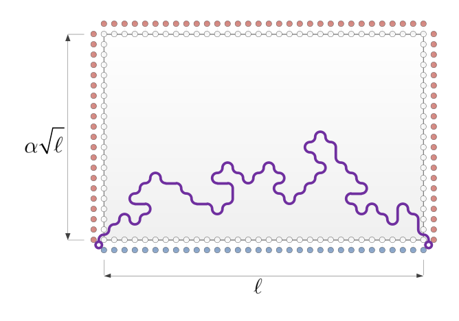
Consider a rectangle with boundary conditions that are identically (+)(+) on the South boundary and (−)(-) elsewhere. The following proposition addresses a large deviation estimate for the vertical fluctuations of the unique open contour in this setting, as illustrated in Figure 6.
Refer to caption
Figure 6. Large deviation estimate for vertical fluctuations of the open Peierls contour under (−,−,+,−)(-,-,+,-) b.c., established in Proposition 4.4.
Proposition 4.4.

Let RR be a rectangle of dimensions ℓ×α​ℓ\ell\times\alpha\sqrt{\ell} with 1<α≤ℓ1<\alpha\leq\sqrt{\ell} and let πR(−,−,+,−)\pi_{R}^{(-,-,+,-)} be the corresponding Ising Gibbs measure with (−,−,+,−)(-,-,+,-) ordered clockwise starting from the North side. Let λ=λ⁡(σ)\lambda=\lambda(\sigma) denote the unique open Peierls contour of the spin configuration σ∈ΩR\sigma\in\Omega_{R}. Then for any β>βc\beta>\beta_{c} there exist constants c1,c2>0c_{1},c_{2}>0 depending only on β\beta such that for any 0<δ<10<\delta<1 and α,ℓ\alpha,\ell as above

πR(−,−,+,−)​(σ:λ⁡(σ)​ reaches height ​δ​α​ℓ)≤ℓc1​e−c2​(δ​α)2.\pi_{R}^{(-,-,+,-)}\Bigl(\sigma:\ \lambda(\sigma)\text{ reaches height }\delta\alpha\sqrt{\ell}\Bigr)\leq\ell^{\,c_{1}}e^{-c_{2}(\delta\alpha)^{2}}\,. (4.4)
Remark.

In the proof of the statement 𝒜⁡(Ln,tn,δn)⇒ℬ⁡(Ln,tn′,δn′)\mathcal{A}(L_{n},t_{n},\delta_{n})\Rightarrow\mathcal{B}(L_{n},t^{\prime}_{n},\delta^{\prime}_{n}) for n∈[N0,N]n\in[N_{0},N], the above proposition is used with ℓ=3​Ln\ell=3L_{n}, α=3​2​κN\alpha=3\sqrt{2}\kappa_{N} and δ=(3​2)−1\delta=(3\sqrt{2})^{-1}. Thus for κ\kappa large enough depending on β\beta and for every n∈[N0,N]n\in[N_{0},N] the r.h.s. of (4.4) is quite small.

The second equilibrium bound that is needed can be formulated as follows. Mark the rectangle RR as given above by the corners (x,y,y′,x′)(x,y,y^{\prime},x^{\prime}) clockwise starting from the Northwest corner. Consider the Ising Gibbs measure on RR with the following b.c.:

  1. (i)

    −1-1 on the North boundary and on an interval Δ\Delta of length s​α2s\alpha^{2} belonging to the South boundary and centered around its midpoint;

  2. (ii)

    +1+1 elsewhere.

We refer to these boundary conditions as the b.c. (−,+,Δ)(-,+,\Delta) and let uu and vv denote the West and East endpoints of the interval Δ\Delta centered on the South border.

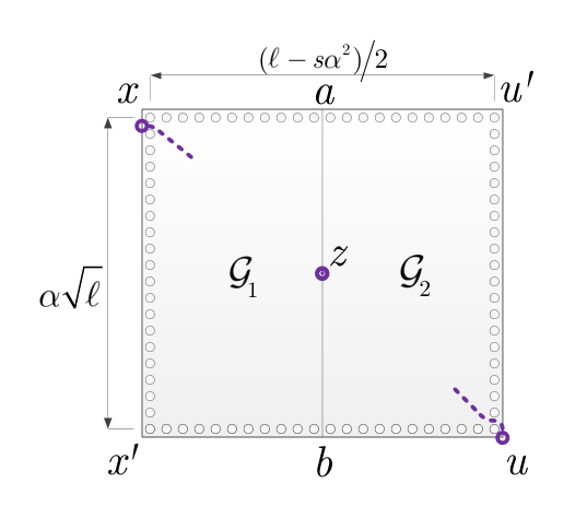
In this new setting we aim to show that w.h.p. in the random-line representation there are two open contours λ1\lambda_{1} and λ2\lambda_{2} with δ​λ1={x,u}\delta\lambda_{1}=\{x,u\} and δ​λ2={y,v}\delta\lambda_{2}=\{y,v\} and such that λ1\lambda_{1} (resp. λ2\lambda_{2}) lies entirely in the left (resp. right) half of RR, as shown in Figure 7 (recall the discussion following Lemma 3.8 for the role of this event in the inductive scheme). This is established by the next proposition.

Refer to caption
Figure 7. Open Peierls contours confined to the left and right halves of the rectangle RR under (−,+,Δ)(-,+,\Delta) b.c., addressed by the equilibrium estimate of Proposition 4.5.
Proposition 4.5.

For any β>βc\beta>\beta_{c} there exist c1,c2,s0>0c_{1},c_{2},s_{0}>0 depending only on β\beta so that the following holds. Let RR be a rectangle of size ℓ×α​ℓ\ell\times\alpha\sqrt{\ell} with 1<α<(1/s0)​ℓ1<\alpha<(1/s_{0})\sqrt{\ell} and let Δ=[u,v]\Delta=[u,v] be an interval of length s​α2s\alpha^{2} centered on the South border for some s≥s0s\geq s_{0}. Let 𝒱\mathcal{V} denote the event that there are two open Peierls contours confined to the left and right halves of RR and connecting the top corners with u,vu,v. Then

π(−,+,Δ)​(𝒱c)≤ℓc1​e−c2​α2.\pi^{(-,+,\Delta)}(\mathcal{V}^{c})\leq\ell^{c_{1}}e^{-c_{2}\alpha^{2}}\,. (4.5)
Remark.

In the proof of the statement ℬ⁡(Ln,tn′,δn′)⇒𝒜⁡(Ln+1,tn+1,δn+1)\mathcal{B}(L_{n},t^{\prime}_{n},\delta^{\prime}_{n})\Rightarrow\mathcal{A}(L_{n+1},t_{n+1},\delta_{n+1}) the above proposition is invoked with a choice of ℓ=Ln\ell=L_{n}, n∈[N0,N]n\in[N_{0},N], and α=2​2​κN\alpha=2\sqrt{2}\kappa_{N}, so that α=o⁡(ℓ)\alpha=o(\sqrt{\ell}); also, the r.h.s. of (4.5) is always very small provided that the constant κ\kappa is chosen to be large enough.

5. Equilibrium crossing probabilities for the infinite strip

In this section we study the behavior of the unique open contour in the infinite strip with boundary conditions (+)(+) in the upper half-plane and (−)(-) in the lower half-plane. Deriving sharp estimates for the probability that this contour is confined to the upper half-plane, as well as a large deviation estimate for the its vertical fluctuations, will later serve as a key element in the proofs of Propositions 4.4 and 4.5. The analysis in this section hinges on the duality tools developed in [40, 39], which enable us to characterize the Ising interfaces for any β>βc\beta>\beta_{c}. By using this machinery together with some additional ideas we establish various properties of the contours, roughly analogous to Brownian bridges with logarithmic “decorations”.

Refer to caption
Figure 8. Infinite strip with mixed b.c. and its unique open contour.

For S⊂ℤ2S\subset\mathbb{Z}^{2} define the boundary condition η∈{±1}ℤ2∖S\eta\in\{\pm 1\}^{\mathbb{Z}^{2}\setminus S} to be

η⁡(x,y)={−1y>0,+1y≤0.\eta(x,y)=\left\{\begin{array}[]{ll}-1&y>0\,,\\ +1&y\leq 0\,.\end{array}\right. (5.1)

We focus on the case where SS is the infinite-strip of width ℓ\ell,

S={1,…,ℓ}×ℤ,S=\{1,\ldots,\ell\}\times\mathbb{Z}\,, (5.2)

whereby the above b.c. η\eta gives rise to a unique open contour λ\lambda connecting the dual vertices {12,12},{ℓ+12,12}\{\frac{1}{2},\frac{1}{2}\},\{\ell+\frac{1}{2},\frac{1}{2}\} in S∗S^{*} (see Figure 8). Such contours have been intensively studied and the scaling limit of λ\lambda is known to be the 1d Brownian bridge between these two points [20] while our proof requires more quantitative estimates. Tight large deviation estimates for vertical fluctuations of λ\lambda are necessary in several places in our proof. This will be established by Theorem 5.3 below (in a slightly more general setting) via an argument akin to those used for controlling the deviations of the Brownian bridge yet carried out within the duality framework of [40, 39].

Significantly more delicate is the crucial estimate of obtaining a lower bound on the probability that λ\lambda is contained in the upper half-plane. The Brownian bridge heuristic suggests that this event holds with probability proportional to 1/ℓ1/\ell, and as the following theorem confirms this is indeed the case.

Theorem 5.1.

Let SS be the infinite strip of width ℓ\ell with b.c. η\eta as given in (5.1),(5.2). For an Ising configuration σ\sigma on SS let λ=λ⁡(σ)\lambda=\lambda(\sigma) be its unique open contour in the dual lattice S∗S^{*} (i.e. δ​λ={(12,12),(ℓ+12,12)}\delta\lambda=\{(\frac{1}{2},\frac{1}{2}),(\ell+\frac{1}{2},\frac{1}{2})\}). For i∈ℤi\in\mathbb{Z} let Hi∗={12,…,ℓ+12}×{i+12}H^{*}_{i}=\{\frac{1}{2},\ldots,\ell+\frac{1}{2}\}\times\{i+\frac{1}{2}\} be the vertices comprising the ii-th horizontal level of S∗S^{*}. Then for every ℓ\ell,

cℓ≤πSη​(σ:λ⁡(σ)​ stays above ​H−1∗)≤Cℓ,\frac{c}{\ell}\leq\pi^{\eta}_{S}\left(\sigma:\,\lambda(\sigma)\mbox{ stays above }H^{*}_{-1}\right)\leq\frac{C}{\ell}\,,

where c,C>0c,C>0 are constants that depend only on β\beta.

As an immediate consequence we obtain the following lower bound on the spin-spin correlation at high temperature for two points on the horizontal boundary of the half-strip S+={12,…,ℓ+12}×ℤ+⁣∗S^{+}=\{\frac{1}{2},\ldots,\ell+\frac{1}{2}\}\times{\mathbb{Z}}^{+*}, which to our knowledge was previously unknown.

Corollary 5.2.

Let u=(12,12)u=(\frac{1}{2},\frac{1}{2}) and v=(ℓ+12,12)v=(\ell+\frac{1}{2},\frac{1}{2}). For every β>βc\beta>\beta_{c} there exist constants c,c′c,c^{\prime} such that

cℓ3/2​e−τβ​(u−v)≤πS+∗​(σu​σv)≤c′ℓ3/2​e−τβ​(u−v).\frac{c}{\ell^{3/2}}e^{-\tau_{\beta}(u-v)}\leq\pi^{*}_{S^{+}}(\sigma_{u}\sigma_{v})\leq\frac{c^{\prime}}{\ell^{3/2}}e^{-\tau_{\beta}(u-v)}\,.

Note that the above corollary also extends to other geometries, for instance rectangles with a wide range of aspect ratios where u,vu,v correspond to the upper corners. We postpone the proof of Theorem 5.1 and Corollary 5.2 in order to first obtain several of the ingredients that it would require, the first of which being the aforementioned large deviation inequality for the open contour in the infinite strip SS.

Theorem 5.3.

Let S¯=S¯​(a,b)\bar{S}=\bar{S}(a,b) be the infinite strip {1,…,ℓ}×ℤ\{1,\ldots,\ell\}\times\mathbb{Z} excluding the horizontal slits {1,…,a}×{0,1}\{1,\ldots,a\}\times\{0,1\} and {b,…,ℓ}×{0,1}\{b,\ldots,\ell\}\times\{0,1\} for 0≤a<b≤ℓ+10\leq a<b\leq\ell+1 with b.c. η\eta as defined in (5.1). For an Ising configuration σ\sigma on S¯\bar{S} let λ=λ⁡(σ)\lambda=\lambda(\sigma) be its unique open contour in the dual S¯∗\bar{S}^{*}, and for i∈ℤi\in\mathbb{Z} let Hi∗={12,…,ℓ+12}×{i+12}H^{*}_{i}=\{\frac{1}{2},\ldots,\ell+\frac{1}{2}\}\times\{i+\frac{1}{2}\}. Then there exist some constant C⁡(β)>0C(\beta)>0 such that for any ℓ\ell the following holds:

πS¯η​(σ:λ⁡(σ)​ reaches ​Hx​ℓ∗)\displaystyle\pi^{\eta}_{\bar{S}}\left(\sigma:\,\lambda(\sigma)\mbox{ reaches }H^{*}_{x\sqrt{\ell}}\right) ≤C​exp⁡(−κβ​x2)\displaystyle\leq C\exp\left(-\kappa_{\beta}\;x^{2}\right) for all x≤ℓ,\displaystyle\mbox{for all $x\leq\sqrt{\ell}$}\,,
πS¯η​(σ:λ⁡(σ)​ reaches ​Hh∗)\displaystyle\pi^{\eta}_{\bar{S}}\Big(\sigma:\,\lambda(\sigma)\mbox{ reaches }H^{*}_{h}\Big) ≤C​exp⁡(−κβ​h)\displaystyle\leq C\exp\left(-\kappa_{\beta}\;h\right) for all h≥ℓ,\displaystyle\mbox{for all $h\geq\ell$}\,,

where κβ>0\kappa_{\beta}>0 is the constant in the sharp triangle inequality of the surface tension τβ\tau_{\beta}.

Remark.

It is fairly straightforward to establish upper bounds as above with an extra prefactor of order |b−a||b-a| (see e.g. the first inequality in (5.12)). Eliminating this spurious prefactor requires a delicate multi-scale analysis.

Proof of theorem.

In what follows we will prove the following inequality, which is a stronger form of the required large deviation estimates: For some C=C⁡(β)>0C=C(\beta)>0,

πS¯η​(σ:λ⁡(σ)​ reaches ​Hh∗)\displaystyle\pi^{\eta}_{\bar{S}}\left(\sigma:\,\lambda(\sigma)\mbox{ reaches }H^{*}_{h}\right) ≤Ce−κβ​(h2b−a−1∧h) for any h>0\displaystyle\leq Ce^{-\kappa_{\beta}\big(\tfrac{h^{2}}{b-a-1}\;\wedge\;h\big)}\quad\mbox{ for any $h>0$} (5.3)

(we may clearly assume that b>a+1b>a+1 otherwise the unique open contour is trivial). Indeed, the above probability estimate is clearly increasing in the value of b−ab-a, which in turn is guaranteed to be at most ℓ+1\ell+1 (reflecting the bounds in the proposition). Notice that by choosing CC to be appropriately large we need only consider h≥b−ah\geq\sqrt{b-a}.

Fix some large cutoff height n≥(h∨ℓ)2n\geq(h\;\vee\;\ell)^{2} and let

S¯n=S¯∩(ℤ×{−n,…,n})\bar{S}_{n}=\bar{S}\cap(\mathbb{Z}\times\{-n,\ldots,n\})

be the strip S¯\bar{S} truncated at ±n\pm n with boundary conditions analogous to η\eta, i.e. negative on the upper half-plane and positive elsewhere. Due to the uniqueness of the Gibbs measure on S¯\bar{S}, the probabilities we seek to bound are obtained as a limit of the corresponding ones for S¯n\bar{S}_{n} as n→∞n\to\infty. Further let u=(a+12,12)u=(a+\frac{1}{2},\frac{1}{2}) and v=(b−12,12)v=(b-\frac{1}{2},\frac{1}{2}) denote the endpoints of the unique open contour in S¯n∗\bar{S}_{n}^{*}. Define the height of this open contour λ⊂S¯n∗\lambda\subset\bar{S}_{n}^{*} at the horizontal coordinate x∈{12,…,ℓ+12}x\in\{\frac{1}{2},\ldots,\ell+\frac{1}{2}\} to be

ht⁡(λ,x)=max⁡{y:(x,y)∈λ}.\operatorname{ht}(\lambda,x)=\max\{y:(x,y)\in\lambda\}\,.

The main effort in the proof will be devoted to the analysis of the vertical fluctuations of the contour λ\lambda within the inner strip with xx-coordinates {a+12,…,b−12}\{a+\frac{1}{2},\ldots,b-\frac{1}{2}\}. It is the case that large vertical fluctuations in the margins (i.e. large values of ht⁡(λ,x)\operatorname{ht}(\lambda,x) for x<ax<a or x>bx>b) are far more unlikely and can be estimated via standard properties of the surface tension. To control the delicate fluctuations of ht⁡(λ,x)\operatorname{ht}(\lambda,x) for a<x<ba<x<b we will apply a multiscale approach, repeatedly bounding the deviations at the horizontal midpoints in a nested dyadic partition of the interval between uu and vv.

The first step in the proof is to bound the event that the contour includes a given point w=(x,h)∈S¯∗w=(x,h)\in\bar{S}^{*} in terms of its coordinates hh and xx. First notice that by (2.8),

πS¯nη(σ:w∈λ(σ))=[∑λ:δ​λ={u,v}w∈λqS¯n∗(λ)]/[∑λ:δ​λ={u,v}qS¯n∗(λ)].\pi^{\eta}_{\bar{S}_{n}}\left(\sigma:\,w\in\lambda(\sigma)\right)=\biggl[\sum_{\begin{subarray}{c}\lambda:\,\delta\lambda=\{u,v\}\\ w\in\lambda\end{subarray}}q_{\bar{S}_{n}^{*}}(\lambda)\biggr]\,\big/\,\biggl[\sum_{\begin{subarray}{c}\lambda:\,\delta\lambda=\{u,v\}\end{subarray}}q_{\bar{S}_{n}^{*}}(\lambda)\biggr]\,. (5.4)

Consider the numerator in the last expression: Corollary 2.5 implies that

∑λ:δ​λ={u,v}w∈λqS¯n∗(λ)≤πS¯n∗∗(σuσw)πS¯∗∗(σvσw),\sum_{\begin{subarray}{c}\lambda:\,\delta\lambda=\{u,v\}\\ w\in\lambda\end{subarray}}q_{\bar{S}_{n}^{*}}(\lambda)\leq\pi_{\bar{S}_{n}^{*}}^{*}\left(\sigma_{u}\,\sigma_{w}\right)\,\pi_{\bar{S}^{*}}^{*}\left(\sigma_{v}\,\sigma_{w}\right)\,,

and together with Lemma 2.1 we deduce that for some c0=c0​(β)>0c_{0}=c_{0}(\beta)>0

∑λ:δ​λ={u,v}w∈λqS¯n∗(λ)\displaystyle\sum_{\begin{subarray}{c}\lambda:\,\delta\lambda=\{u,v\}\\ w\in\lambda\end{subarray}}q_{\bar{S}_{n}^{*}}(\lambda) ≤c0|u−w|​|v−w|​exp⁡(−τβ​(u−w)−τβ​(v−w)).\displaystyle\leq\frac{c_{0}}{\sqrt{|u-w||v-w|}}\exp\big(-\tau_{\beta}(u-w)-\tau_{\beta}(v-w)\big)\,. (5.5)

To estimate the denominator in (5.4) recall Eq. (2.7) according to which

∑λ:δ​λ={u,v}qS¯n∗(λ)=πS¯n∗∗(σuσv).\sum_{\begin{subarray}{c}\lambda:\,\delta\lambda=\{u,v\}\end{subarray}}q_{\bar{S}_{n}^{*}}(\lambda)=\pi_{\bar{S}_{n}^{*}}^{*}(\sigma_{u}\,\sigma_{v})\,.

As it follows from GKS that decreasing our domain can only decrease the spin-spin correlations, letting Sn={a,…,b}×{−n,…,n}S_{n}=\{a,\ldots,b\}\times\{-n,\ldots,n\} (i.e. SnS_{n} is the result of “pushing” the West and East boundaries of S¯n\bar{S}_{n} to aa and bb resp.) we have

πS¯n∗∗​(σu​σv)≥πSn∗∗​(σu​σv).\pi_{\bar{S}_{n}^{*}}^{*}(\sigma_{u}\,\sigma_{v})\geq\pi_{S_{n}^{*}}^{*}(\sigma_{u}\,\sigma_{v})\,.

By Eq. (2.3) there exists some c1=c1​(β)>0c_{1}=c_{1}(\beta)>0 such that the spin-spin correlation between u,vu,v in the dual to the infinite strip S={a,…,b}×ℤS=\{a,\ldots,b\}\times\mathbb{Z} is

πS∗∗​(σu​σv)=c1+o⁡(1)|u−v|​exp⁡(−τβ​(|u−v|)),\pi_{S^{*}}^{*}(\sigma_{u}\,\sigma_{v})=\frac{c_{1}+o(1)}{\sqrt{|u-v|}}\exp(-\tau_{\beta}(|u-v|))\,,

where the o⁡(1)o(1)-term tends to 00 as |u−v|→∞|u-v|\to\infty. Due to the strong spatial mixing properties of the high temperature region β∗<βc\beta^{*}<\beta_{c}, the value of πSn∗∗​(σu​σv)\pi_{S_{n}^{*}}^{*}(\sigma_{u}\,\sigma_{v}) converges to the above r.h.s. exponentially fast in nn. Already for n≥ℓ2n\geq\ell^{2} we could absorb the error in the constant c1c_{1} and obtain that for some c1′​(β)>0c^{\prime}_{1}(\beta)>0,

∑λ:δ​λ={u,v}qS¯n∗(λ)≥c1′|u−v|exp(−τβ(|u−v|)).\sum_{\begin{subarray}{c}\lambda:\,\delta\lambda=\{u,v\}\end{subarray}}q_{\bar{S}_{n}^{*}}(\lambda)\geq\frac{c^{\prime}_{1}}{\sqrt{|u-v|}}\exp(-\tau_{\beta}(|u-v|))\,. (5.6)

By combining (5.4) with (5.5) and (5.6) we conclude that for some c2=c2​(β)>0c_{2}=c_{2}(\beta)>0,

πS¯nη(σ:w∈λ(σ))≤c2​|u−v||u−w|​|v−w|exp(−τβ(u−w)−τβ(v−w)+τβ(u−v)).\pi^{\eta}_{\bar{S}_{n}}\left(\sigma:\,w\in\lambda(\sigma)\right)\leq\frac{c_{2}\sqrt{|u-v|}}{\sqrt{|u-w||v-w|}}\exp\left(-\tau_{\beta}(u-w)-\tau_{\beta}(v-w)+\tau_{\beta}(u-v)\right)\,. (5.7)

At the same time, by the sharp triangle inequality property (2.2) of the surface tension,

τβ​(u−w)\displaystyle\tau_{\beta}(u-w) +τβ​(v−w)≥τβ​(u−v)+κβ​(|w−v|+|u−w|−|u−v|).\displaystyle+\tau_{\beta}(v-w)\geq\tau_{\beta}(u-v)+\kappa_{\beta}\left(|w-v|+|u-w|-|u-v|\right)\,. (5.8)

Recalling that ww is at height hh it is easy to verify that

|w−v|+|u−w|−|u−v|≥4​h2|u−v|2+4​h2+|u−v|.|w-v|+|u-w|-|u-v|\geq\frac{4h^{2}}{\sqrt{|u-v|^{2}+4h^{2}}+|u-v|}\,.

Set ξ=41+5>65\xi=\frac{4}{1+\sqrt{5}}>\frac{6}{5} and now observe that whenever h2≤|u−v|2h^{2}\leq|u-v|^{2} the last expression is at least ξ​h2|u−v|\xi\tfrac{h^{2}}{|u-v|} and otherwise it is at least ξ​h\xi h. Using this bound for the r.h.s. of Eq. (5.8) now allows us to produce the following bound out of Eq. (5.7):

πS¯nη(σ:w∈λ(σ))≤c2​|u−v||u−w|​|v−w|exp(−65κβ(h2|u−v|∧h)).\pi^{\eta}_{\bar{S}_{n}}\left(\sigma:\,w\in\lambda(\sigma)\right)\leq\frac{c_{2}\sqrt{|u-v|}}{\sqrt{|u-w||v-w|}}\exp\left(-\tfrac{6}{5}\kappa_{\beta}\left(\tfrac{h^{2}}{|u-v|}\;\wedge\;h\right)\right)\,. (5.9)

Straightforward applications of the above bounds will now yield the required bounds on the height of λ\lambda along the margins x≤a+12x\leq a+\frac{1}{2} and x≥b−12x\geq b-\frac{1}{2} as well as whenever b−ab-a is a uniformly bounded. Indeed, by symmetry we may assume without loss of generality that x≤a+12x\leq a+\frac{1}{2} and note that in this case w=(x,h)w=(x,h) satisfies |w−v|≥|u−v||w-v|\geq|u-v|. Applying (5.7) combined with the sharp triangle inequality as in Eq. (5.8) we get

πS¯nη(σ:w∈λ(σ))≤c2|u−w|exp(−κβ|u−w|).\pi^{\eta}_{\bar{S}_{n}}\left(\sigma:\,w\in\lambda(\sigma)\right)\leq\frac{c_{2}}{\sqrt{|u-w|}}\exp\left(-\kappa_{\beta}|u-w|\right)\,.

Summing the last expression over all w=(x,y)w=(x,y) with x≤a+12x\leq a+\frac{1}{2} and y≥hy\geq h gives that

πS¯nη(σ:ht(λ(σ),x)≥h for some x≤a+12)≤C1e−κβ​h\pi^{\eta}_{\bar{S}_{n}}\big(\sigma:\,\operatorname{ht}(\lambda(\sigma),x)\geq h\mbox{ for some $x\leq a+\tfrac{1}{2}$}\big)\leq C_{1}\,e^{-\kappa_{\beta}h} (5.10)

for some C1=C1​(β)>0C_{1}=C_{1}(\beta)>0, and analogously

πS¯nη(σ:ht(λ(σ),x)≥h for some x≥b−12)≤C1e−κβ​h.\pi^{\eta}_{\bar{S}_{n}}\big(\sigma:\,\operatorname{ht}(\lambda(\sigma),x)\geq h\mbox{ for some $x\geq b-\tfrac{1}{2}$}\big)\leq C_{1}\,e^{-\kappa_{\beta}h}\,. (5.11)

We now turn our attention to the main task of bounding the vertical fluctuations of λ\lambda along the interval (a+12,b−12)(a+\frac{1}{2},b-\frac{1}{2}). First observe that (5.9) immediately provides the bound we seek (Eq. (5.3)) in the special case where |u−v|=O⁡(1)|u-v|=O(1) (with an implicit constant that may depend on β\beta): In that case a simple union bound over w=(x,h)w=(x,h) for x∈(a+12,b−12)x\in(a+\frac{1}{2},b-\frac{1}{2}) yields

πS¯nη(σ:\displaystyle\pi^{\eta}_{\bar{S}_{n}}\big(\sigma:\, OPENht⁡(λ⁡(σ),x)≥h​ for some a+12<x<b−12)\displaystyle\operatorname{ht}(\lambda(\sigma),x)\geq h\mbox{ for some $a+\tfrac{1}{2}<x<b-\tfrac{1}{2}$}\big)
≤c2​|u−v|​exp⁡(−65​κβ​(h2|u−v|∧h))≤C2​exp⁡(−κβ​(h2|u−v|∧h)),\displaystyle\leq c_{2}|u-v|\exp\left(-\tfrac{6}{5}\kappa_{\beta}\left(\tfrac{h^{2}}{|u-v|}\;\wedge\;h\right)\right)\leq C_{2}\,\exp\left(-\kappa_{\beta}\left(\tfrac{h^{2}}{|u-v|}\;\wedge\;h\right)\right)\,, (5.12)

where C2​(β)>0C_{2}(\beta)>0 incorporates the uniform bound on |u−v||u-v|. Combined with (5.10) and (5.11) this concludes the bound in Eq. (5.3) when |u−v|=O⁡(1)|u-v|=O(1).

Let M≥2M\geq 2 be some fixed integer whose value will depend only on β\beta and will be specified later. Justified by the above argument, assume without loss of generality that

|u−v|≥M2 and exp⁡(110​κβ​|u−v|1/4)≥|u−v|.|u-v|\geq M^{2}\quad\mbox{ and }\quad\exp\Big(\tfrac{1}{10}\kappa_{\beta}|u-v|^{1/4}\Big)\geq|u-v|\,. (5.13)

We claim that this in turn narrows our attention to proving Eq. (5.3) for hh satisfying

M​|u−v|≤h2≤12​|u−v|5/4.M|u-v|\leq h^{2}\leq\tfrac{1}{2}|u-v|^{5/4}\,. (5.14)

To see this recall first that the lower bound on hh is justified by selecting a suitably large constant C⁡(β)C(\beta) in Eq. (5.3). For the upper bound, note that if h2>12​|u−v|5/4h^{2}>\frac{1}{2}|u-v|^{5/4} (in which case h2|u−v|>12​|u−v|1/4\tfrac{h^{2}}{|u-v|}>\frac{1}{2}|u-v|^{1/4} whereas h>12​|u−v|5/8h>\frac{1}{\sqrt{2}}|u-v|^{5/8}) then (5.13) implies that |u−v||u-v| is at most exp⁡(κβ5​(h2|u−v|∧h))\exp\left(\frac{\kappa_{\beta}}{5}\big(\tfrac{h^{2}}{|u-v|}\;\wedge\;h\big)\right) and hence Eq. (5.3) follows from a union bound over x∈(a+12,b−12)x\in(a+\frac{1}{2},b-\frac{1}{2}) as in (5.12).

Consider the event whereby the contour λ\lambda visits a point w∈S¯nw\in\bar{S}_{n} given by

w=(x,y)​ for some ​x∈(a+1M​|u−v|,b−1M​|u−v|)​ and ​y≥h.w=(x,y)\mbox{ for some }x\in\left(a+\tfrac{1}{M}|u-v|,b-\tfrac{1}{M}|u-v|\right)\mbox{ and }y\geq h\,.

Clearly |u−w|​|v−w|≥1M​|u−v|\sqrt{|u-w||v-w|}\geq\tfrac{1}{M}|u-v| thus we can rewrite (5.9) as

πS¯nη(σ:w∈λ(σ))≤c3|u−v|exp(−65κβ(y2|u−v|∧y)),\pi^{\eta}_{\bar{S}_{n}}\left(\sigma:\,w\in\lambda(\sigma)\right)\leq\frac{c_{3}}{\sqrt{|u-v|}}\exp\left(-\tfrac{6}{5}\kappa_{\beta}\left(\tfrac{y^{2}}{|u-v|}\;\wedge\;y\right)\right)\,,

where c3>0c_{3}>0 depends only on β\beta. Summing over all possible values of y≥hy\geq h we now obtain that

πS¯nη\displaystyle\pi^{\eta}_{\bar{S}_{n}} (σ:ht(λ(σ),x)≥h)≤c3|u−v|(∑y=h|u−v|e−65​κβ​y2|u−v|+∑y≥(h∨|u−v|)e−65​κβ​y)\displaystyle\Big(\sigma:\,\operatorname{ht}\left(\lambda(\sigma),x\right)\geq h\Big)\leq\frac{c_{3}}{\sqrt{|u-v|}}\bigg(\sum_{y=h}^{|u-v|}e^{-\tfrac{6}{5}\kappa_{\beta}\,\tfrac{y^{2}}{|u-v|}}+\sum_{y\geq(h\;\vee\;|u-v|)}\!\!e^{-\tfrac{6}{5}\kappa_{\beta}\,y}\bigg)
≤c3​∑z=h/|u−v||u−v|e−65​κβ​z2+c3|u−v|​∑y≥he−65​κβ​y≤c3′​e−65​κβ​h2|u−v|+c3′|u−v|​e−65​κβ​h\displaystyle\leq c_{3}\sum_{z=h/\sqrt{|u-v|}}^{\sqrt{|u-v|}}e^{-\tfrac{6}{5}\kappa_{\beta}z^{2}}+\frac{c_{3}}{\sqrt{|u-v|}}\sum_{y\geq h}e^{-\tfrac{6}{5}\kappa_{\beta}\,y}\leq c_{3}^{\prime}e^{-\tfrac{6}{5}\kappa_{\beta}\frac{h^{2}}{|u-v|}}+\frac{c^{\prime}_{3}}{\sqrt{|u-v|}}e^{-\tfrac{6}{5}\kappa_{\beta}h}
≤C3​exp⁡(−65​κβ​(h2|u−v|∧h)),\displaystyle\leq C_{3}\,\exp\left(-\tfrac{6}{5}\kappa_{\beta}\left(\tfrac{h^{2}}{|u-v|}\;\wedge\;h\right)\right)\,, (5.15)

where the constant C3>0C_{3}>0 depends only on β\beta.

We next wish to extend the above bound on ht⁡(λ,x)\operatorname{ht}(\lambda,x) to hold simultaneously for all x∈(a+12,b−12)x\in(a+\frac{1}{2},b-\frac{1}{2}) by means of a dyadic partition of the interval between uu and vv. Set

K=⌊12​logM​|u−v|⌋K=\Big\lfloor\frac{1}{2}\log_{M}|u-v|\Big\rfloor

and notice that (5.13) ensures that K≥1K\geq 1. Define the following sequence of refinements of the interval between uu and vv, indexed by k=0,…,Kk=0,\ldots,K. We begin with the trivial partition at level 00,

z0(0)=a+12,\displaystyle z_{0}^{(0)}=a+\tfrac{1}{2}\,, z1(0)=b−12,\displaystyle\quad z_{1}^{(0)}=b-\tfrac{1}{2}\,,

and refine level kk into level k+1k+1 by subdividing each subinterval (zj−1(k),zj(k))(z_{j-1}^{(k)},z_{j}^{(k)}) into MM equal parts (up to integer rounding):

zM​j(k+1)\displaystyle z_{Mj}^{(k+1)} =zj(k)\displaystyle=z_{j}^{(k)} for ​j=0,…,Mk,\displaystyle\mbox{ for }j=0,\ldots,M^{k}\,,
zM⁡(j−1)+i(k+1)\displaystyle z_{M(j-1)+i}^{(k+1)} =⌊zj−1(k)+iM​(zj−1(k)+zj(k))⌋+12\displaystyle=\left\lfloor z_{j-1}^{(k)}+\tfrac{i}{M}\big(z_{j-1}^{(k)}+z_{j}^{(k)}\big)\right\rfloor+\tfrac{1}{2} for ​i=1,…,M−1​ and ​j=1,…,Mk.\displaystyle\mbox{ for }i=1,\ldots,M-1\mbox{ and }j=1,\ldots,M^{k}\,.

Observe that for all admissible j,kj,k we have

M−k​|u−v|−2<zj(k)−zj−1(k)<M−k​|u−v|+2,M^{-k}|u-v|-2<z_{j}^{(k)}-z_{j-1}^{(k)}<M^{-k}|u-v|+2\,,

where the additive terms account for the rounding corrections along the refinements. In particular, the expression in the lower bound on the sub-interval lengths satisfies

M−k​|u−v|≥M−K​|u−v|≥|u−v|>10M^{-k}|u-v|\geq M^{-K}|u-v|\geq\sqrt{|u-v|}>10

(as |u−v||u-v| is large enough). Next, define

hk=M−k/4h\displaystyle h_{k}=M^{-k/4}h  for k=0,…,K,\displaystyle\quad\mbox{ for $k=0,\ldots,K$}\,,

and let Υj(k)\Upsilon_{j}^{(k)} be the event that the height of the contour at zj(k)z_{j}^{(k)} does not exceed ∑i<khi\sum_{i<k}h_{i}:

Υj(k)={σ:ht⁡(λ⁡(σ),zj(k))<∑i=0k−1hi}​ for k≥1 and 1≤j<Mk.\Upsilon_{j}^{(k)}=\bigg\{\sigma:\,\operatorname{ht}\big(\lambda(\sigma),z_{j}^{(k)}\big)<\sum_{i=0}^{k-1}h_{i}\bigg\}\mbox{ for $k\geq 1$ and $1\leq j<M^{k}$}\,.

Recalling (5.15) and rewriting it in terms of Υj(k)\Upsilon_{j}^{(k)} and its complement Υ¯j(k)\overline{\Upsilon}_{j}^{(k)} we have that

πS¯nη​(Υ¯j(1))≤C3​exp⁡(−65​κβ​(h02z1(0)−z0(0)∧h0))​ for j=1,…,M−1.\pi^{\eta}_{\bar{S}_{n}}\left(\overline{\Upsilon}_{j}^{(1)}\right)\leq C_{3}\,\exp\bigg(-\tfrac{6}{5}\kappa_{\beta}\bigg(\frac{h_{0}^{2}}{z^{(0)}_{1}-z^{(0)}_{0}}\;\wedge\;h_{0}\bigg)\bigg)\mbox{ for $j=1,\ldots,M-1$}\,.

Exactly the same argument yields that for general kk, 1≤j≤Mk1\leq j\leq M^{k} and 1≤i≤M−11\leq i\leq M-1,

πS¯nη​(Υ¯M⁡(j−1)+i(k+1),Υj−1(k),Υj(k))≤C3​exp⁡(−65​κβ​(hk2zj(k)−zj−1(k)∧hk)).\pi^{\eta}_{\bar{S}_{n}}\left(\overline{\Upsilon}^{(k+1)}_{M(j-1)+i}\,,\,\Upsilon^{(k)}_{j-1}\,,\,\Upsilon^{(k)}_{j}\right)\leq C_{3}\,\exp\bigg(-\tfrac{6}{5}\kappa_{\beta}\bigg(\frac{h_{k}^{2}}{z^{(k)}_{j}-z^{(k)}_{j-1}}\;\wedge\;h_{k}\bigg)\bigg)\,. (5.16)

To estimate the last expression, observe that hk/(zj(k)−zj−1(k))h_{k}/(z_{j}^{(k)}-z_{j-1}^{(k)}) increases with kk roughly as M3​k/4M^{3k/4}. More accurately,

hkzj(k)−zj−1(k)≤Mk4​hM−k​|u−v|−2≤M3​k4​h|u−v|​(1+2M−k​|u−v|−2)<54​M3​k4​h|u−v|\displaystyle\frac{h_{k}}{z_{j}^{(k)}-z_{j-1}^{(k)}}\leq\frac{M^{\frac{k}{4}}h}{M^{-k}|u-v|-2}\leq\frac{M^{\frac{3k}{4}}h}{|u-v|}\Big(1+\frac{2}{M^{-k}|u-v|-2}\Big)<\frac{5}{4}M^{\frac{3k}{4}}\frac{h}{|u-v|} (5.17)

(where we used the fact that M−k​|u−v|>10M^{-k}|u-v|>10) and similarly

hkzj(k)−zj−1(k)≥Mk4​hM−k​|u−v|+2>45​M3​k4​h|u−v|.\displaystyle\frac{h_{k}}{z_{j}^{(k)}-z_{j-1}^{(k)}}\geq\frac{M^{\frac{k}{4}}h}{M^{-k}|u-v|+2}>\frac{4}{5}M^{\frac{3k}{4}}\frac{h}{|u-v|}\,. (5.18)

Our choice of KK and the upper bound (5.14) on hh enable us to derive from (5.17) that for all k≤Kk\leq K,

hkzj(k)−zj−1(k)≤54M3​K/412|u−v|−3/8≤54​2<1.\frac{h_{k}}{z_{j}^{(k)}-z_{j-1}^{(k)}}\leq\frac{5}{4}M^{3K/4}\frac{1}{\sqrt{2}}|u-v|^{-3/8}\leq\frac{5}{4\sqrt{2}}<1\,.

In particular, this identifies the minimizer of the exponent in the r.h.s. of (5.16) and implies that

πS¯nη​(Υ¯M⁡(j−1)+i(k+1),Υj−1(k),Υj(k))≤C3​exp⁡(−65​κβ​hk2zj(k)−zj−1(k)).\pi^{\eta}_{\bar{S}_{n}}\left(\overline{\Upsilon}^{(k+1)}_{M(j-1)+i}\,,\,\Upsilon^{(k)}_{j-1}\,,\,\Upsilon^{(k)}_{j}\right)\leq C_{3}\,\exp\bigg(-\tfrac{6}{5}\kappa_{\beta}\frac{h_{k}^{2}}{z^{(k)}_{j}-z^{(k)}_{j-1}}\bigg)\,.

Crucially however, the lower bound (5.18) also gives that

hk2zj(k)−zj−1(k)≥45M3​k/4h|u−v|M−k/4h=45Mk/2h2|u−v|.\frac{h^{2}_{k}}{z_{j}^{(k)}-z_{j-1}^{(k)}}\geq\frac{4}{5}M^{3k/4}\frac{h}{|u-v|}M^{-k/4}h=\frac{4}{5}M^{k/2}\frac{h^{2}}{|u-v|}\,.

To simplify the notation put ρ=65​κβ​h2|u−v|\rho=\frac{6}{5}\kappa_{\beta}\frac{h^{2}}{|u-v|} and recall that ρ≥65​κβ​M\rho\geq\frac{6}{5}\kappa_{\beta}M by (5.14), hence we may take MM sufficiently large so ρ\rho would also be large. The combination of the above inequalities together with a union bound gives

πS¯nη​(⋃k=1K−1⋃jΥ¯j(k))\displaystyle\pi^{\eta}_{\bar{S}_{n}}\bigg(\bigcup_{k=1}^{K-1}\bigcup_{j}\overline{\Upsilon}^{(k)}_{j}\bigg) =πS¯nη​(⋃k=1K−1⋃i,j{Υ¯M⁡(j−1)+i(k),Υj−1(k−1),Υj(k−1)})\displaystyle=\pi^{\eta}_{\bar{S}_{n}}\bigg(\bigcup_{k=1}^{K-1}\bigcup_{i,j}\left\{\overline{\Upsilon}^{(k)}_{M(j-1)+i}\,,\,\Upsilon^{(k-1)}_{j-1}\,,\,\Upsilon^{(k-1)}_{j}\right\}\bigg)
≤C3​M​e−ρ+C3​∑k=2K−1Mk​e−ρ​45​M(k−1)/2≤C3′​e−ρ=C3′​e65​κβ​h2|u−v|,\displaystyle\leq C_{3}Me^{-\rho}+C_{3}\sum_{k=2}^{K-1}M^{k}e^{-\rho\,\frac{4}{5}M^{(k-1)/2}}\leq C^{\prime}_{3}e^{-\rho}=C^{\prime}_{3}e^{\frac{6}{5}\kappa_{\beta}\frac{h^{2}}{|u-v|}}\,,

where we used that ρ≥2\rho\geq 2 and M≥log⁡M\sqrt{M}\geq\log M for any sufficiently large MM and it is understood that Υj(0)\Upsilon^{(0)}_{j} is the full probability space.

We have reached level KK at which point we wish to examine the remaining points altogether. Fix some x∈(zj−1(K−1),zj(K−1))x\in(z_{j-1}^{(K-1)},z_{j}^{(K-1)}) and let

Υx′={σ:ht⁡(λ⁡(σ),x)<∑i=1Khi}.\Upsilon^{\prime}_{x}=\bigg\{\sigma:\,\operatorname{ht}\big(\lambda(\sigma),x\big)<\sum_{i=1}^{K}h_{i}\bigg\}\,.

As established before hK/(zj(K)−zj−1(K))<1h_{K}/(z_{j}^{(K)}-z_{j-1}^{(K)})<1 and so

πS¯nη​(Υ¯x′,Υj−1(K),Υj(K))≤C3​exp⁡(−65​κβ​hK2zj(K)−zj−1(K)).\pi^{\eta}_{\bar{S}_{n}}\left(\overline{\Upsilon}^{\prime}_{x}\,,\,\Upsilon^{(K)}_{j-1}\,,\,\Upsilon^{(K)}_{j}\right)\leq C_{3}\,\exp\bigg(-\tfrac{6}{5}\kappa_{\beta}\frac{h_{K}^{2}}{z^{(K)}_{j}-z^{(K)}_{j-1}}\bigg)\,. (5.19)

On the other hand, by the definition of KK we have that MK≥|u−v|1/2/MM^{K}\geq|u-v|^{1/2}/M (with the factor of MM due to possible integer rounding in KK) and hence

hK2zj(K)−zj−1(K)\displaystyle\frac{h^{2}_{K}}{z_{j}^{(K)}-z_{j-1}^{(K)}} ≥45​MK/2​h2|u−v|≥45​|u−v|1/4M​h2|u−v|≥|u−v|1/4,\displaystyle\geq\frac{4}{5}M^{K/2}\frac{h^{2}}{|u-v|}\geq\frac{4}{5}\frac{|u-v|^{1/4}}{\sqrt{M}}\frac{h^{2}}{|u-v|}\geq|u-v|^{1/4}\,,

where the last inequality is due to the lower bound on h2h^{2} in (5.14). It now follows from (5.13) that

exp⁡(−110​κβ​hK2zj(K)−zj−1(K))≤exp⁡(−110​κβ​|u−v|1/4)≤|u−v|−1.\exp\bigg(-\tfrac{1}{10}\kappa_{\beta}\frac{h_{K}^{2}}{z^{(K)}_{j}-z^{(K)}_{j-1}}\bigg)\leq\exp\left(-\tfrac{1}{10}\kappa_{\beta}|u-v|^{1/4}\right)\leq|u-v|^{-1}\,.

Together with (5.19) this implies that

πS¯nη​(Υ¯x′,Υj−1(K),Υj(K))≤C3|u−v|​exp⁡(−1110​κβ​h2|u−v|).\pi^{\eta}_{\bar{S}_{n}}\left(\overline{\Upsilon}^{\prime}_{x}\,,\,\Upsilon^{(K)}_{j-1}\,,\,\Upsilon^{(K)}_{j}\right)\leq\frac{C_{3}}{|u-v|}\,\exp\bigg(-\tfrac{11}{10}\kappa_{\beta}\frac{h^{2}}{|u-v|}\bigg)\,.

Summing over at most |u−v||u-v| possible choices for xx we may now conclude that

πS¯nη​(ht⁡(λ,x)≥αM​h​ for some x∈(a+12,b−12))≤C4​exp⁡(−1110​κβ​h2|u−v|),\displaystyle\pi^{\eta}_{\bar{S}_{n}}\left(\operatorname{ht}(\lambda,x)\geq\alpha_{M}h\mbox{ for some $x\in(a+\tfrac{1}{2},b-\tfrac{1}{2})$}\right)\leq C_{4}\exp\bigg(-\tfrac{11}{10}\kappa_{\beta}\frac{h^{2}}{|u-v|}\bigg)\,, (5.20)

where αM=∑0KM−i/4<(1−M−1/4)−1\alpha_{M}=\sum_{0}^{K}M^{-i/4}<\big(1-M^{-1/4}\big)^{-1}.

Finally, by choosing MM to be sufficiently large we can obtain that αM2<1110\alpha_{M}^{2}<\frac{11}{10} and plugging this in (5.20) (while recalling that we are in the regime where h2|u−v|≤h\tfrac{h^{2}}{|u-v|}\leq h due to Eq. (5.14)) concludes the proof of (5.3), as required. ∎

Remark.

The truncation argument that was used in the proof of Theorem 5.3 to reduce the problem to a finite domain is applicable in our upcoming arguments as well. Henceforth, when needed, we will thus work directly in the infinite volume setting to simplify the exposition.

We now introduce the main conceptual element in the proof of Theorem 5.1. Recall our aim is to show that the open contour in the infinite strip S={1,…,ℓ}×ℤS=\{1,\ldots,\ell\}\times\mathbb{Z} has a reasonable probability — namely of order c/ℓc/\ell — of remaining in the upper half-plane (i.e. above the dual line {(x,y):y=−12}\{(x,y):y=-\frac{1}{2}\}).

Our approach, based on the Brownian bridge heuristics, is iterative and very much based on the intuitive picture in which the open contour really consists of two simple lines γ1,γ2\gamma_{1},\ \gamma_{2}, traveled at constant speed, one starting from the left boundary and moving towards the right boundary and viceversa for the second one, meeting in some intermediate point. Such a picture, which can be made more precise by progressively revealing the contour from the left to right and from right to left (see Figure 9), allows hitting times kind of arguments that we now explain. Let τj(i)\tau_{j}^{(i)} (i=1,2i=1,2) be the hitting time of either level 00 or level 2j2^{j} for the curve γi\gamma_{i}. Then, conditioned to the event that both curves at their respective times τj(i)\tau_{j}^{(i)} have not yet joined and are both at level 2j2^{j}, by monotonicity and symmetry, with probability at least 1/41/4 both curves will either hit the next level 2j+12^{j+1} or join together before hitting level 00 (see Claim 5.8 below for a precise formulation). Thus, with probability at least 4−n4^{-n} we can force both curves to either hit level 2n2^{n} or join together before hitting level 00. However, and that explains the heuristic bound 1/ℓ1/\ell, once the curves are at level 2n≈ℓ2^{n}\approx\sqrt{\ell}, then with probability bounded away from 00 they will join together without hitting level 00. In other words it is enough to force the curves to climb only n=12​log2​ℓn=\frac{1}{2}\log_{2}\ell levels in order not to hit level 00.

The above sketch, however, suppresses a number of technical difficulties such as the boundary conditions and the dependence between the two contours. Moreover, and contrary to the behavior of the Brownian bridge, the law of the contour λ\lambda is in fact asymmetric w.r.t. the horizontal axis. This follows from our splitting-rule, which introduces a vertical bias for the contour: For instance, as illustrated in Figure 10, applying the SE splitting-rule clearly has the open contour move up with probability uniformly bounded away from 12\frac{1}{2}.

Refer to caption
Figure 9. The open contour in the infinite strip with mixed b.c., progressively exposed as two curves γ1,γ2\gamma_{1},\gamma_{2} originating at its endpoints.
Figure 10. Asymmetric behavior of the contour due to the global SE splitting-rule.

To overcome this difficulty we consider the open contours formed by both the SE and the SW splitting-rules, γse\gamma_{\textsc{se}} and γsw\gamma_{\textsc{sw}} resp., and examine their union Γ=γse∪γsw\Gamma=\gamma_{\textsc{se}}\cup\gamma_{\textsc{sw}}. Most importantly the law of their union is symmetric w.r.t. the horizontal axis. We will show that Γ\Gamma is essentially a “tube” of logarithmic width surrounding γse\gamma_{\textsc{se}}, with added “decorations” from γsw\gamma_{\textsc{sw}} which are components of at most logarithmic diameter (and similarly if we reverse the roles of γse,γsw\gamma_{\textsc{se}},\gamma_{\textsc{sw}}). Up to these logarithmic corrections we may implement the heuristics of our above sketch, as stated in the following lemmas. Here and in what follows we associate with an open contour γ\gamma going from uu to vv a unit speed parametrization γ⁡(t)\gamma(t), justifying hitting-time type of events (e.g. “γ\gamma hits the vertex yy prior to hitting zz” etc.).

Lemma 5.4.

Let S¯=S¯​(a,b)\bar{S}=\bar{S}(a,b) and Hi∗H^{*}_{i} (𝑂𝑃𝐸𝑁i∈ℤ)i\in\mathbb{Z}) be as in Theorem 5.3. For an Ising configuration σ\sigma on S¯\bar{S} let γse​(σ)\gamma_{\textsc{se}}(\sigma) and γsw​(σ)\gamma_{\textsc{sw}}(\sigma) be the two unique open contours in S¯∗\bar{S}^{*} formed by the SE and SW splitting-rules resp., i.e. going from (a+12,12)(a+\frac{1}{2},\frac{1}{2}) to (b−12,12)(b-\frac{1}{2},\frac{1}{2}). There exists some C⋆​(β)>0C^{\star}(\beta)>0 so that for any h≥1h\geq 1 the contour γse\gamma_{\textsc{se}} (resp. γsw\gamma_{\textsc{sw}}) hits H−h−C⋆​log⁡h∗H^{*}_{-h-C^{\star}\log h} before hitting either Hh−C⋆​log⁡h∗H^{*}_{h-C^{\star}\log h} or (b−12,12)(b-\frac{1}{2},\frac{1}{2}) with probability at most 12+C⋆/h\frac{1}{2}+C^{\star}/h.

Proof.

We define the gain of a connected subset of dual edges AA in the infinite strip S¯\bar{S} in the interval I⊂ℤI\subset\mathbb{Z} over distance mm, denoted by gn⁡(A,I,m)\operatorname{gn}(A,I,m), to be the maximal difference in yy-coordinates between any two points in AA whose xx-coordinates are contained in II and differ by at most mm:

gn(A,I,m):=maxx,y,x′,y′{|y−y′|:|x−x′|≤m,(x,y)∈A,(x′,y′)∈A,x,x′∈I}.\operatorname{gn}(A,I,m):=\max_{x,y,x^{\prime},y^{\prime}}\left\{|y-y^{\prime}|:|x-x^{\prime}|\leq m,(x,y)\in A,\,(x^{\prime},y^{\prime})\in A,x,x^{\prime}\in I\right\}\,. (5.21)

We define the gradient of AA as its gain over distance 0. The following claim bounds the gain of γ\gamma in a neighborhood of aa and bb:

Claim 5.5.

Let γ\gamma be the open contour with either SE or SW splitting-rule in the infinite strip S¯=S¯​(a,b)\bar{S}=\bar{S}(a,b) of side-length ℓ\ell defined in Theorem 5.3. Then for any c>0c>0 there exists a constant C1⋆=C1⋆​(β,c)>0C^{\star}_{1}=C^{\star}_{1}(\beta,c)>0 such that for all 1≤m≤ℓ1\leq m\leq\ell,

πS¯η​(gn⁡(γ,[a−m,a+m],c​log⁡m)>C1⋆​log⁡m)≤C1⋆/m.\pi^{\eta}_{\bar{S}}\Big(\operatorname{gn}(\gamma,[a-m,a+m],c\log m)>C^{\star}_{1}\log m\Big)\leq C^{\star}_{1}/m\,.

The analogous statement holds replacing aa with bb.

Proof of Claim 5.5.

Define I=[a−m,a+m]∩ℤI=[a-m,a+m]\cap{\mathbb{Z}} and in what follows take C1⋆≥cC_{1}^{\star}\geq c. Further let u=(a+12,12)u=(a+\frac{1}{2},\frac{1}{2}) and v=(b−12,12)v=(b-\frac{1}{2},\frac{1}{2}) denote the endpoints of the open contour γ\gamma, and let C1⋆=C1⋆​(β)C^{\star}_{1}=C^{\star}_{1}(\beta) be some constant to be determined later. Define the set

Ξ={((x,y),(x′,y′))∈S¯2:x,x′∈I,|x−x′|≤clogm,|y−y′|≥C1⋆logm}.\Xi=\{((x,y),(x^{\prime},y^{\prime}))\in\bar{S}^{2}:x,x^{\prime}\in I,|x-x^{\prime}|\leq c\log m,|y-y^{\prime}|\geq C^{\star}_{1}\log m\}\,.

If gn⁡(γ,I,c​log⁡m)>C1⋆​log⁡m\operatorname{gn}(\gamma,I,c\log m)>C^{\star}_{1}\log m then there exist z=(x,y),z′=(x′,y′)∈γz=(x,y),z^{\prime}=(x^{\prime},y^{\prime})\in\gamma such that (z,z′)∈Ξ(z,z^{\prime})\in\Xi. Taking a union bound over ordered pairs of intermediate points z,z′∈Ξz,z^{\prime}\in\Xi such that z=(x,y)z=(x,y) and z′=(x′,y′)z^{\prime}=(x^{\prime},y^{\prime}) we get that

πS¯η(gn(γ,I,clogm)>C1⋆logm)≤[∑(z,z′)∈Ξ∑λ:δ​λ={u,v}z,z′∈λqS¯∗(λ)]/[∑λ:δ​λ={u,v}qS¯∗(λ)].\pi^{\eta}_{\bar{S}}\Big(\operatorname{gn}(\gamma,I,c\log m)>C^{\star}_{1}\log m\Big)\leq\biggl[\sum_{\begin{subarray}{c}(z,z^{\prime})\in\Xi\end{subarray}}\sum_{\begin{subarray}{c}\lambda:\,\delta\lambda=\{u,v\}\\ z,z^{\prime}\in\lambda\end{subarray}}q_{\bar{S}^{*}}(\lambda)\biggr]\,\big/\,\biggl[\sum_{\begin{subarray}{c}\lambda:\,\delta\lambda=\{u,v\}\end{subarray}}q_{\bar{S}^{*}}(\lambda)\biggr]\,.

As we have already seen, Eq. (2.3) provides a sharp estimate for the above denominator and it remains to consider the numerator. Recall Corollary 2.5 that treated the measure of all open contours λ\lambda in a domain Λ∗\Lambda^{*} that go between two endpoints u,vu,v as well as an intermediate point zz, bounding it from above by the product of the spin-spin correlations πΛ∗∗​(σu​σz)\pi_{\Lambda^{*}}^{*}\left(\sigma_{u}\,\sigma_{z}\right) and πΛ∗∗​(σv​σz)\pi_{\Lambda^{*}}^{*}\left(\sigma_{v}\,\sigma_{z}\right). Following essentially the same proof, [39]*Lemma 5.4 gives an analogous version of this statement for all such contours λ\lambda going through two ordered intermediate points z,z′z,z^{\prime} (that is, γ\gamma connects uu to zz, thereafter proceeds to z′z^{\prime} and ends at vv) whereby

∑λ:δ​λ={u,v}z,z′∈λqΛ∗(λ)\displaystyle\sum_{\begin{subarray}{c}\lambda:\,\delta\lambda=\{u,v\}\\ z,z^{\prime}\in\lambda\end{subarray}}q_{\Lambda^{*}}(\lambda) ≤πΛ∗∗​(σu​σz)​πΛ∗∗​(σz​σz′)​πΛ∗∗​(σz′​σv).\displaystyle\leq\pi_{\Lambda^{*}}^{*}\left(\sigma_{u}\,\sigma_{z}\right)\,\pi_{\Lambda^{*}}^{*}\left(\sigma_{z}\,\sigma_{z^{\prime}}\right)\,\pi_{\Lambda^{*}}^{*}\left(\sigma_{z^{\prime}}\,\sigma_{v}\right)\,. (5.22)

Therefore, Lemma 2.1 implies that

∑λ:δ​λ={u,v}z,z′∈λqS¯∗(λ)≤Cβ3​exp⁡(−[τβ​(u−z)+τβ​(z−z′)+τβ​(v−z′)])|u−z|⋅|z−z′|⋅|z′−v|.\sum_{\begin{subarray}{c}\lambda:\,\delta\lambda=\{u,v\}\\ z,z^{\prime}\in\lambda\end{subarray}}q_{\bar{S}^{*}}(\lambda)\leq\frac{C_{\beta}^{3}\exp\big(-[\tau_{\beta}(u-z)+\tau_{\beta}(z-z^{\prime})+\tau_{\beta}(v-z^{\prime})]\big)}{\sqrt{|u-z|\cdot|z-z^{\prime}|\cdot|z^{\prime}-v|}}\,.

Since τβ​(θ)≥τβ​(0)\tau_{\beta}(\theta)\geq\tau_{\beta}(0) (see e.g. [6]) we can bound the last exponent from above by

e−τβ​(0)​[|u−z|+|z−z′|+|v−z′|]≤e−τβ​(0)​[|u−v|+c′​(|y|/m+|y−y′|)],e^{-\tau_{\beta}(0)[|u-z|+|z-z^{\prime}|+|v-z^{\prime}|]}\leq e^{-\tau_{\beta}(0)[|u-v|+c^{\prime}(|y|/m+|y-y^{\prime}|)]}\,,

where c′>0c^{\prime}>0 is an absolute constant; indeed, the last inequality is justified by the fact that |y−y′||y-y^{\prime}| is at least a constant times |x−x′||x-x^{\prime}| (recall that C1∗≥cC_{1}^{*}\geq c) and a similar statement holds w.r.t. y/my/m compared to |x−a||x-a|. Since summing over x,x′x,x^{\prime} amounts to a factor of O⁡(m2)O(m^{2}), absorbing an additional O⁡(m)O(m) term from the sum over y/my/m while recalling that |y−y′|≥C1⋆​log⁡m|y-y^{\prime}|\geq C_{1}^{\star}\log m now implies that

∑λ:δ​λ={u,v}z,z′∈λqS¯∗(λ)≤Cm−p|u−v|−1/2exp(−τβ(u−v)),\sum_{\begin{subarray}{c}\lambda:\,\delta\lambda=\{u,v\}\\ z,z^{\prime}\in\lambda\end{subarray}}q_{\bar{S}^{*}}(\lambda)\leq Cm^{-p}|u-v|^{-1/2}\exp(-\tau_{\beta}(u-v))\,,

where pp can be made arbitrarily large by taking C1⋆C_{1}^{\star} large enough. In conclusion,

πS¯η​(gn⁡(γ,I,c​log⁡m)>C1⋆​log⁡m)≤C1⋆/m,\pi^{\eta}_{\bar{S}}\Big(\operatorname{gn}(\gamma,I,c\log m)>C^{\star}_{1}\log m\Big)\leq C_{1}^{\star}/m\,,

completing the proof. ∎

Claim 5.6.

Let γse\gamma_{\textsc{se}} and γsw\gamma_{\textsc{sw}} be the open contours with the SE and SW splitting-rule resp. in the infinite strip S¯=S¯​(a,b)\bar{S}=\bar{S}(a,b) of side-length ℓ\ell defined in Theorem 5.3. Then there exists some C2⋆=C2⋆​(β)>0C^{\star}_{2}=C^{\star}_{2}(\beta)>0 so that for all 1≤m≤ℓ1\leq m\leq\ell with probability at least 1−C2⋆/m1-C^{\star}_{2}/m every connected component of γsw∖γse\gamma_{\textsc{sw}}\setminus\gamma_{\textsc{se}} with zero distance from ([a−m,a+m]×ℤ)∩γse([a-m,a+m]\times\mathbb{Z})\cap\gamma_{\textsc{se}} has diameter at most C2⋆​log⁡mC^{\star}_{2}\log m.

Proof of Claim 5.6.

Let ℬ\mathcal{B} denote the event that there exists a connected component of γsw∖γse\gamma_{\textsc{sw}}\setminus\gamma_{\textsc{se}} with zero distance from ([a−m,a+m]×ℤ)∩γse([a-m,a+m]\times\mathbb{Z})\cap\gamma_{\textsc{se}} and has diameter at least C2⋆​log⁡mC^{\star}_{2}\log m. We begin by conditioning on γse\gamma_{\textsc{se}}. The contour partitions S¯\bar{S} into two sets StopS_{\textsc{top}} and SbotS_{\textsc{bot}}. For a set of dual edges AA let V⁡(A)⊂ℤ2V(A)\subset\mathbb{Z}^{2} denote the set of vertices at distance 12\frac{1}{2} from AA. The effect of conditioning on γse\gamma_{\textsc{se}} is equivalent to conditioning that σU=ηU\sigma_{U}=\eta_{U} where U=V⁡(Δ⁡(γse))U=V(\Delta(\gamma_{\textsc{se}})) (recall the definition of the edge-boundary Δ⁡(⋅)\Delta(\cdot) in §2 after Lemma 2.2) and ηU∈{−1,+1}U\eta_{U}\in\{-1,+1\}^{U} is the configuration given by

ηu={−1u∈Stop,+1u∈Sbot.\eta_{u}=\begin{cases}-1&u\in S_{\textsc{top}},\\ +1&u\in S_{\textsc{bot}}.\end{cases}

Conditional on γse\gamma_{\textsc{se}} the configuration σ\sigma on S¯∖U\bar{S}\setminus U is given by the Ising model on Stop∖US_{\textsc{top}}\setminus U and Sbot∖US_{\textsc{bot}}\setminus U with minus and plus boundary conditions respectively. Let θ\theta denote the ensemble of contours of this configuration given by the SW (not SE!) splitting rule. Since the boundary conditions are all minus and all plus there are no open contours. Every maximal connected segment of γsw∖γse\gamma_{\textsc{sw}}\setminus\gamma_{\textsc{se}} must be a subset of one of the closed contours of θ\theta and must share a common vertex with γse\gamma_{\textsc{se}}.

By Theorem 5.3 we see that γse∪γsw⊂Λ∗\gamma_{\textsc{se}}\cup\gamma_{\textsc{sw}}\subset\Lambda^{*} where Λ={1,…,ℓ}×{−ℓ,…,ℓ}\Lambda=\{1,\ldots,\ell\}\times\{-\ell,\ldots,\ell\} except with probability O⁡(exp⁡(−c​ℓ))O(\exp(-c\ell)) for some c⁡(β)>0c(\beta)>0. By Claim 5.5 there are at most 2​C1⋆​m​log⁡m2C^{\star}_{1}m\log m vertices in ℐ=([a−m,a+m]×ℤ)∩γse\mathcal{I}=([a-m,a+m]\times\mathbb{Z})\cap\gamma_{\textsc{se}} except with probability C1⋆/mC_{1}^{\star}/m. For z,z′∈Λ∗z,z^{\prime}\in\Lambda^{*} the probability that both lie in the same closed contour of θ\theta is at most exp⁡(−τβ​(z−z′))\exp(-\tau_{\beta}(z-z^{\prime})) by Lemma 2.6. Since the surface tension achieves its minimum on the sphere at τβ​(0)>0\tau_{\beta}(0)>0 [6] combining the above estimates we have that

πS¯η​(ℬ)\displaystyle\pi^{\eta}_{\bar{S}}\left(\mathcal{B}\right) ≤Cexp(−cℓ)+C1⋆/m+∑z∈ℐ∑z′:|z−z′|>C2⋆​log⁡mexp(−|z−z′|τβ(0))\displaystyle\leq C\exp(-c\ell)+C_{1}^{\star}/m+\sum_{z\in\mathcal{I}}~\sum_{z^{\prime}:|z-z^{\prime}|>C_{2}^{\star}\log m}\exp(-|z-z^{\prime}|\tau_{\beta}(0))
≤C​exp⁡(−c​ℓ)+C1⋆/m+C​m1−C2⋆​τβ​(0)​log3​m,\displaystyle\leq C\exp(-c\ell)+C_{1}^{\star}/m+Cm^{1-C_{2}^{\star}\tau_{\beta}(0)}\log^{3}m\,,

The desired result follows from a sufficiently large choice of C2⋆C^{\star}_{2}. ∎

Finally we show that the contours γse\gamma_{\textsc{se}} and γsw\gamma_{\textsc{sw}} are unlikely to travel much farther than h2h^{2} in the xx-coordinate before attaining height hh or −h-h.

Lemma 5.7.

Let S¯=S¯​(a,b)\bar{S}=\bar{S}(a,b). For any w>0w>0 and 0<h≤ℓ0<h\leq\ell define the rectangle

ℛ={a−12−w,…,a−12+w}×{12−h,…,h+12}.\mathcal{R}=\{a-\tfrac{1}{2}-w,\ldots,a-\tfrac{1}{2}+w\}\times\{\tfrac{1}{2}-h,\ldots,h+\tfrac{1}{2}\}\,.

Let ℬ\mathcal{B} denote the event that the contour γse\gamma_{\textsc{se}} (resp. γsw\gamma_{\textsc{sw}}) beginning at (a−12,12)(a-\frac{1}{2},\frac{1}{2}) exits ℛ\mathcal{R} and the first point it hits in ℛc\mathcal{R}^{c} is in {a−12−w−1,a−12+w+1}×{12−h,…,h+12}\{a-\frac{1}{2}-w-1,a-\frac{1}{2}+w+1\}\times\{\frac{1}{2}-h,\ldots,h+\frac{1}{2}\}. There exists a constant C3⋆​(β)>0C^{\star}_{3}(\beta)>0 independent of ww and hh such that

πS¯η(ℬ)≤C3⋆exp(−w/(C3⋆h2)).\pi^{\eta}_{\bar{S}}\left(\mathcal{B}\right)\leq C^{\star}_{3}\exp\big(-w/(C_{3}^{\star}h^{2})\big)\,.
Proof.

As before let u=(a+12,12)u=(a+\frac{1}{2},\frac{1}{2}) and v=(b−12,12)v=(b-\frac{1}{2},\frac{1}{2}) denote the endpoints of the open contour γ\gamma. Let ℬr\mathcal{B}_{r} and ℬl\mathcal{B}_{l} denote the events that the contour exits to the right and left of ℛ\mathcal{R} respectively so that ℬ=ℬl∪ℬr\mathcal{B}=\mathcal{B}_{l}\cup\mathcal{B}_{r}. We will examine the case that the contour exits to the right and the left case will follow similarly. Fix c⁡(β)=(3​e​Cβ)2c(\beta)=(3eC_{\beta})^{2} where CβC_{\beta} is the constant in Lemma 2.1. For large enough C3⋆C_{3}^{\star} the bound holds trivially when w≤2​c​h2w\leq 2ch^{2} so assume that w>2​c​h2w>2ch^{2}. We may define M⁡(w,h)∈ℤM(w,h)\in\mathbb{Z} such that 0<w/(4​c​h2)≤M⁡(w,h)≤w/(c​h2)0<w/(4ch^{2})\leq M(w,h)\leq w/(ch^{2}) and |c​M​h2−(b−a)|≥12​|b−a||cMh^{2}-(b-a)|\geq\frac{1}{2}|b-a|. Define the set of sequences of points

Ξ={(x1,y1),…,(xM,yM)∈S¯M:∀i,xi=a+12+ich2,|yi|≤h}\Xi=\{(x_{1},y_{1}),\ldots,(x_{M},y_{M})\in\bar{S}^{M}:\forall i,\ x_{i}=a+\tfrac{1}{2}+ich^{2},|y_{i}|\leq h\}

and note that if the contour exits ℛ\mathcal{R} to the right then it must pass from uu through a sequence of points in Ξ\Xi in order and then to bb. For a sequence ξ∈Ξ\xi\in\Xi we say that λ\lambda is ξ\xi-admissible if it passes through the points in ξ\xi in order and then returns to bb. Note also that by the construction of MM we have that |xM−(b−12)|≥12​|b−a||x_{M}-(b-\frac{1}{2})|\geq\frac{1}{2}|b-a|. Taking a union bound over sequences in Ξ\Xi we get that

πS¯η(ℬR)≤[∑ξ∈Ξ∑λ:δ​λ={u,v}ξ−admissibleqS¯∗(λ)]/[∑λ:δ​λ={u,v}qS¯∗(λ)].\pi^{\eta}_{\bar{S}}\Big(\mathcal{B}_{R}\Big)\leq\biggl[\sum_{\begin{subarray}{c}\xi\in\Xi\end{subarray}}\sum_{\begin{subarray}{c}\lambda:\,\delta\lambda=\{u,v\}\\ \xi-\text{admissible}\end{subarray}}q_{\bar{S}^{*}}(\lambda)\biggr]\,\big/\,\biggl[\sum_{\begin{subarray}{c}\lambda:\,\delta\lambda=\{u,v\}\end{subarray}}q_{\bar{S}^{*}}(\lambda)\biggr]\,.

In analogy to Corollary 2.5 and (5.22) one has

∑λ:δ​λ={u,v}ξ−admissibleqΛ∗(λ)\displaystyle\sum_{\begin{subarray}{c}\lambda:\,\delta\lambda=\{u,v\}\\ \xi-\text{admissible}\end{subarray}}q_{\Lambda^{*}}(\lambda) ≤∏i=1M+1πΛ∗∗​(σ(xi,yi)​σ(xi−1,yi−1)),\displaystyle\leq\prod_{i=1}^{M+1}\pi_{\Lambda^{*}}^{*}\left(\sigma_{(x_{i},y_{i})}\,\sigma_{(x_{i-1},y_{i-1})}\right)\,,

where we denote u=(x0,y0)u=(x_{0},y_{0}) and v=(xM+1,yM+1)v=(x_{M+1},y_{M+1}). Therefore, Lemma 2.1 implies that

∑λ:δ​λ={u,v}ξ−admissibleqS¯∗(λ)\displaystyle\sum_{\begin{subarray}{c}\lambda:\,\delta\lambda=\{u,v\}\\ \xi-\text{admissible}\end{subarray}}q_{\bar{S}^{*}}(\lambda) ≤CβM+1exp(−∑i=1M+1τβ((xi,yi)−(xi−1,yi−1)))∏i=1M+1|(xi,yi)−(xi−1,yi−1)|\displaystyle\leq\frac{C_{\beta}^{M+1}\exp\big(-\sum_{i=1}^{M+1}\tau_{\beta}((x_{i},y_{i})-(x_{i-1},y_{i-1}))\big)}{\sqrt{\prod_{i=1}^{M+1}|(x_{i},y_{i})-(x_{i-1},y_{i-1})|}}
≤Cβ​exp⁡(−M−τβ​(u−v))(3​h)M​12​|b−a|.\displaystyle\leq C_{\beta}\frac{\exp\big(-M-\tau_{\beta}(u-v)\big)}{(3h)^{M}\sqrt{\frac{1}{2}|b-a|}}\,.

Summing over the (2​h+1)M(2h+1)^{M} elements of Ξ\Xi we have that

∑ξ∈Ξ∑λ:δ​λ={u,v}ξ−admissibleqS¯∗(λ)≤Cβexp⁡(−M−τβ​(u−v))12​|b−a|.\sum_{\begin{subarray}{c}\xi\in\Xi\end{subarray}}\sum_{\begin{subarray}{c}\lambda:\,\delta\lambda=\{u,v\}\\ \xi-\text{admissible}\end{subarray}}q_{\bar{S}^{*}}(\lambda)\leq C_{\beta}\frac{\exp\big(-M-\tau_{\beta}(u-v)\big)}{\sqrt{\frac{1}{2}|b-a|}}\,.

and it follows (recall Eq. 2.3) that there exists a constant C⁡(β)>0C(\beta)>0 such that

πS¯η​(ℬR)≤C​e−M\pi^{\eta}_{\bar{S}}\left(\mathcal{B}_{R}\right)\leq Ce^{-M}\,

and a similar estimate holds for πS¯η​(ℬL)\pi^{\eta}_{\bar{S}}\left(\mathcal{B}_{L}\right). Recalling that M≥w/(4​c​h2)M\geq w/(4ch^{2}) and taking a suitably large C3⋆C^{\star}_{3} now completes the proof. ∎

We now complete the proof of Lemma 5.4. Recalling that Γ=γse∪γsw\Gamma=\gamma_{\textsc{se}}\cup\gamma_{\textsc{sw}} we define Γtop\Gamma_{\textsc{top}} to be the highest path in Γ\Gamma connecting (a+12,12)(a+\frac{1}{2},\frac{1}{2}) to (b−12,12)(b-\frac{1}{2},\frac{1}{2}). First observe that Γtop\Gamma_{\textsc{top}} is indeed well defined. The collection of dual edges Γ\Gamma partitions S¯\bar{S} into two infinite components and possibly a number of finite components. To construct Γtop\Gamma_{\textsc{top}}, view the upper infinite component as a subset of ℝ2\mathbb{R}^{2} by drawing a unit square centered at each of its points. Then Γtop\Gamma_{\textsc{top}} is its “horizontal” boundary connecting (a+12,12)(a+\frac{1}{2},\frac{1}{2}) to (b−12,12)(b-\frac{1}{2},\frac{1}{2}). Define Γbot\Gamma_{\textsc{bot}} similarly as the lowest path in Γ\Gamma. Then

πS¯​(Γtop​ hits H−h∗ before hitting Hh∗ or (b−12,12))\displaystyle\pi_{\bar{S}}\left(\Gamma_{\textsc{top}}\mbox{ hits $H^{*}_{-h}$ before hitting $H^{*}_{h}$ or $(b-\frac{1}{2},\frac{1}{2})$}\right)
≤πS¯​(Γbot​ hits H−h∗ before hitting Hh∗ or (b−12,12))\displaystyle\qquad\leq\pi_{\bar{S}}\left(\Gamma_{\textsc{bot}}\mbox{ hits $H^{*}_{-h}$ before hitting $H^{*}_{h}$ or $(b-\frac{1}{2},\frac{1}{2})$}\right)
=πS¯​(Γtop​ hits Hh∗ before hitting H−h∗ or (b−12,12)),\displaystyle\qquad=\pi_{\bar{S}}\left(\Gamma_{\textsc{top}}\mbox{ hits $H^{*}_{h}$ before hitting $H^{*}_{-h}$ or $(b-\frac{1}{2},\frac{1}{2})$}\right)\,, (5.23)

where the inequality follows by the fact that Γtop\Gamma_{\textsc{top}} lies above Γbot\Gamma_{\textsc{bot}} while the equality is by the symmetry of Γ\Gamma. It follows that

πS¯​(Γtop​ hits H−h∗ before hitting Hh∗ or (b−12,12))≤12.\pi_{\bar{S}}\left(\Gamma_{\textsc{top}}\mbox{ hits $H^{*}_{-h}$ before hitting $H^{*}_{h}$ or $(b-\frac{1}{2},\frac{1}{2})$}\right)\leq\frac{1}{2}\,.

Lemma 5.7 guarantees that except with probability O⁡(exp⁡(−h2))O(\exp(-h^{2})) both contours γse\gamma_{\textsc{se}} and γsw\gamma_{\textsc{sw}} hit either H−h−C⋆​log⁡h∗H^{*}_{-h-C^{\star}\log h} or Hh−C⋆​log⁡h∗H^{*}_{h-C^{\star}\log h} before traveling distance order h4h^{4} in the horizontal direction, and as such we only need to consider the interval [a−h4,a+h4][a-h^{4},a+h^{4}]. Now set

C⋆:=8​C1⋆​(β,C2⋆)+4​C2⋆​(β)C^{\star}:=8C^{\star}_{1}(\beta,C^{\star}_{2})+4C^{\star}_{2}(\beta)

where C1⋆,C2⋆C^{\star}_{1},C^{\star}_{2} are the constants from Claim 5.5 and Claim 5.6. This guarantees that

gn⁡(γse,[a−h4,a+h4],4​C2⋆​log⁡h)\displaystyle\operatorname{gn}\left(\gamma_{\textsc{se}},[a-h^{4},a+h^{4}],4C_{2}^{\star}\log h\right) ≤4​C1⋆​(β,4​C2⋆)​log⁡h,\displaystyle\leq 4C^{\star}_{1}(\beta,4C^{\star}_{2})\log h\,,
gn⁡(γsw,[a−h4,a+h4],4​C2⋆​log⁡h)\displaystyle\operatorname{gn}\left(\gamma_{\textsc{sw}},[a-h^{4},a+h^{4}],4C_{2}^{\star}\log h\right) ≤4​C1⋆​(β,4​C2⋆)​log⁡h,\displaystyle\leq 4C^{\star}_{1}(\beta,4C^{\star}_{2})\log h\,,
max(x,y)∈γswx∈[a−h4,a+h4]⁡d⁡((x,y),γse)\displaystyle\max_{\begin{subarray}{c}(x,y)\in\gamma_{\textsc{sw}}\\ x\in[a-h^{4},a+h^{4}]\end{subarray}}d\left((x,y),\gamma_{\textsc{se}}\right) ≤4​C2⋆​log⁡h\displaystyle\leq 4C^{\star}_{2}\log h

and similarly around bb with probability at least 1−C⋆/h1-C^{\star}/h. In particular, given the above event we have that the vertical distance between Γtop\Gamma_{\textsc{top}} and γse\gamma_{\textsc{se}} does not exceed C⋆​log⁡hC^{\star}\log h in the intervals [a−h4,a+h4][a-h^{4},a+h^{4}] and [b−h4,b+h4][b-h^{4},b+h^{4}] which together with Eq. (5.23) completes the proof. ∎

Proof of Theorem 5.1, lower bound.

The proof proceeds by progressively revealing the contour γse\gamma_{\textsc{se}}. Let w0w_{0} denote some large constant and let wi=2​wi−1−2​C⋆​log⁡wi−1w_{i}=2w_{i-1}-2C^{\star}\log w_{i-1} where C⋆C^{\star} is the constant from Lemma 5.4. Taking w0w_{0} sufficiently large it is easily confirmed that wj≥c​2jw_{j}\geq c2^{j} for some constant c>0c>0.

Starting from the left at (12,12)(\frac{1}{2},\frac{1}{2}) for j≥0j\geq 0 let Al,jA_{l,j} be the event that γse\gamma_{\textsc{se}} hits Hwj∗H^{*}_{w_{j}} before hitting H−1∗H^{*}_{-1} or reaching (ℓ+12,12)(\ell+\frac{1}{2},\frac{1}{2}). Similarly starting from the right at (ℓ+12,12)(\ell+\frac{1}{2},\frac{1}{2}) let Ar,jA_{r,j} be the event that the contour hits Hwj∗H^{*}_{w_{j}} before hitting H−1∗H^{*}_{-1} or reaching (12,12)(\frac{1}{2},\frac{1}{2}). Let Aj=Al,j∩Ar,jA_{j}=A_{l,j}\cap A_{r,j} and let BjB_{j} be the event that the contour γse\gamma_{\textsc{se}} hits neither H−1∗H^{*}_{-1} nor Hwj∗H^{*}_{w_{j}}.

We begin by giving a crude lower bound on the probability of A0A_{0}. Let 𝒰\mathcal{U} be the event that the spin configuration takes the value (+)(+) for all the vertices (1,j)(1,j) and (ℓ,j)(\ell,j) for 0≤j≤w0+10\leq j\leq w_{0}+1. This occurs with probability at least

πS​(𝒰)≥(12​e−8​β)2​w0+2.\pi_{S}(\mathcal{U})\geq(\tfrac{1}{2}e^{-8\beta})^{2w_{0}+2}\,.

On the event 𝒰\mathcal{U} the contour γse​(σ)\gamma_{\textsc{se}}(\sigma) directly passes from (12,12)(\frac{1}{2},\frac{1}{2}) to (12,w0+12)(\frac{1}{2},w_{0}+\frac{1}{2}) and from (ℓ+12,12)(\ell+\frac{1}{2},\frac{1}{2}) to (ℓ+12,w0+12)(\ell+\frac{1}{2},w_{0}+\frac{1}{2}). It follows that 𝒰⊂A0\mathcal{U}\subset A_{0} and hence,

πS​(A0)≥(12​e−8​β)2​w0+2,\pi_{S}(A_{0})\geq(\tfrac{1}{2}e^{-8\beta})^{2w_{0}+2}\,, (5.24)

so in particular A0A_{0} occurs with constant probability.

We will establish the following claim.

Claim 5.8.

There exists a constant c>0c>0 such that for all j≥0j\geq 0 we have that

πS​(Aj+1∪Bj+1∣Aj)≥14−c​2−j.\pi_{S}(A_{j+1}\cup B_{j+1}\mid A_{j})\geq\frac{1}{4}-c2^{-j}.

If we assume the claim then

πS​(Aj+1)+πS​(Bj+1)\displaystyle\pi_{S}(A_{j+1})+\pi_{S}(B_{j+1}) =πS​(Aj+1∩Aj)+πS​(Bj+1∩Aj)+πS​(Bj)\displaystyle=\pi_{S}(A_{j+1}\cap A_{j})+\pi_{S}(B_{j+1}\cap A_{j})+\pi_{S}(B_{j})
≥(14−c​2−j)​[πS​(Aj)+πS​(Bj)]\displaystyle\geq\Big(\frac{1}{4}-c2^{-j}\Big)\left[\pi_{S}(A_{j})+\pi_{S}(B_{j})\right]

where the first inequality follows from the fact that AjA_{j} and BjB_{j} are disjoint. Hence by induction and equation (5.24) we have that for any fixed positive integer KK

P⁡(AK+12​log2​ℓ)+P⁡(BK+12​log2​ℓ)≥P⁡(A0)​∏j=1K+12​log2​ℓ(14−c​2−j)≥c′​4−K​ℓ−1.P(A_{K+\frac{1}{2}\log_{2}\ell})+P(B_{K+\frac{1}{2}\log_{2}\ell})\geq P(A_{0})\prod_{j=1}^{K+\frac{1}{2}\log_{2}\ell}\Big(\frac{1}{4}-c2^{-j}\Big)\geq c^{\prime}4^{-K}\ell^{-1}\,. (5.25)

We now prove the Claim 5.8. Note that if σ′≥σ\sigma^{\prime}\geq\sigma then the curve γse​(σ′)\gamma_{\textsc{se}}(\sigma^{\prime}) must lie on or above γse​(σ)\gamma_{\textsc{se}}(\sigma) and hence the event Aj+1A_{j+1} is increasing in σ\sigma and so is Aj+1∪Bj+1A_{j+1}\cup B_{j+1}. Through a series of monotonicity arguments we will relate this event to that in Lemma 5.4. Suppose that AjA_{j} holds and that the left part of γse\gamma_{\textsc{se}} first hits Hwj∗H_{w_{j}}^{*} at dual vertex (zjL+12,wj+12)(z^{L}_{j}+\frac{1}{2},w_{j}+\frac{1}{2}) and denote this part of the contour by γjL\gamma^{L}_{j}. Similarly denote the right part of the contour as γjR\gamma^{R}_{j} from (ℓ+12,12)(\ell+\frac{1}{2},\frac{1}{2}) to (zjR+12,wj+12)(z^{R}_{j}+\frac{1}{2},w_{j}+\frac{1}{2}) with 12≤zjL<zjR≤ℓ+12\frac{1}{2}\leq z^{L}_{j}<z^{R}_{j}\leq\ell+\frac{1}{2}. Finally, let Dj+1D_{j+1} denote the event that the contour γse\gamma_{\textsc{se}} running between (zjL+12,wj+12)(z^{L}_{j}+\frac{1}{2},w_{j}+\frac{1}{2}) and (zjR+12,wj+12)(z^{R}_{j}+\frac{1}{2},w_{j}+\frac{1}{2}) either hits Hwj+1∗H^{*}_{w_{j+1}} at both ends before hitting H−1∗H^{*}_{-1} or hits neither Hwj+1∗H^{*}_{w_{j+1}} nor H−1∗H^{*}_{-1}. With these definitions we claim that

πS​(Aj+1∪Bj+1∣Aj)≥πSj​(Dj+1∣σUj=ηUj),\displaystyle\pi_{S}\left(A_{j+1}\cup B_{j+1}\mid A_{j}\right)\geq\pi^{j}_{S}\left(D_{j+1}\mid\sigma_{{U}_{j}}={\eta}_{{U}_{j}}\right)\,, (5.26)

where πSj\pi_{S}^{j} denote the measure on the strip SS with boundary condition given by (+)(+) up to wjw_{j} and (−)(-) above wjw_{j},

Uj=([1,zjL+1]∪[zjR,ℓ])×{wj,wj+1}{U_{j}}=\left([1,z^{L}_{j}+1]\cup[z^{R}_{j},\ell]\right)\times\{w_{j},w_{j}+1\}

and

η(u1,u2)={+1u2=wj,−1u2=wj+1.{\eta}_{(u_{1},u_{2})}=\begin{cases}+1&u_{2}=w_{j},\\ -1&u_{2}=w_{j}+1\,.\end{cases}

The sequence of monotonicity arguments establishing (5.26) is best explained schematically, see Fig. 11 and its caption.

Figure 11. Monotonicity transformations to reduce the two segments of the open contour in the infinite strip to the setting of Lemma 5.4. First (top-right) impose extra (−)(-) spins at height wj+1w_{j}+1, making the increasing event Aj+1∪Bj+1A_{j+1}\cup B_{j+1} more unlikely. Next (bottom-right) set the spins at height wjw_{j} and above the contours γjL,γjR\gamma_{j}^{L},\gamma_{j}^{R} to (+)(+); this does not change the probability of Aj+1∪Bj+1A_{j+1}\cup B_{j+1} due to the Markov property of the Gibbs measure. Finally (bottom-left) remove the constraint that the spins just below γjL,γjR\gamma_{j}^{L},\gamma_{j}^{R} are (+)(+), again making the event Aj+1∪Bj+1A_{j+1}\cup B_{j+1} more unlikely. The dotted line is at height wj+1/2w_{j}+1/2.

Let Dj+1LD^{L}_{j+1} denote the event that the contour γse\gamma_{\textsc{se}} from (zjL+12,wj+12)(z^{L}_{j}+\frac{1}{2},w_{j}+\frac{1}{2}) (resp. (zjR+12,wj+12)(z^{R}_{j}+\frac{1}{2},w_{j}+\frac{1}{2})) hits Hwj+1∗H^{*}_{w_{j+1}} or (zjR+12,wj+12)(z^{R}_{j}+\frac{1}{2},w_{j}+\frac{1}{2}) (resp. (zjL+12,wj+12)(z^{L}_{j}+\frac{1}{2},w_{j}+\frac{1}{2})) before hitting H−1∗H^{*}_{-1}. Clearly Dj+1=Dj+1L∩Dj+1RD_{j+1}=D^{L}_{j+1}\cap D^{R}_{j+1} and by symmetry we have that

πSj​(Dj+1L∣σUj=ηUj)=πSj​(Dj+1R∣σUj=ηUj).\pi^{j}_{S}\left(D^{L}_{j+1}\mid\sigma_{{U}_{j}}={\eta}_{{U}_{j}}\right)=\pi^{j}_{S}\left(D^{R}_{j+1}\mid\sigma_{{U}_{j}}={\eta}_{{U}_{j}}\right)\,.

Since these events are both monotone, by the FKG inequality we have that

πSj​(Dj+1∣σUj=ηUj)≥πSj​(Dj+1L∣σUj=ηUj)2.\pi^{j}_{S}\left(D_{j+1}\mid\sigma_{{U}_{j}}={\eta}_{{U}_{j}}\right)\geq\pi^{j}_{S}\left(D^{L}_{j+1}\mid\sigma_{{U}_{j}}={\eta}_{{U}_{j}}\right)^{2}\,.

It finally suffices to note that the conditional event Dj+1LD^{L}_{j+1} is exactly the event considered in Lemma 5.4 once we shift the strip down by wjw_{j} and set h=wj−C⋆​log⁡wjh=w_{j}-C^{\star}\log w_{j}, a=zjLa=z^{L}_{j} and b=zjR−1b=z^{R}_{j}-1. Then we have that

πSj​(Dj+1L∣σUj=ηUj)≥12−O⁡(1/wj)≥12−c​2−j,\pi^{j}_{S}\left(D^{L}_{j+1}\mid\sigma_{{U}_{j}}={\eta}_{{U}_{j}}\right)\geq\frac{1}{2}-O(1/w_{j})\geq\frac{1}{2}-c2^{-j}\,,

which completes the proof of Claim 5.8.

To complete the proof of the lower bound in Theorem 5.1 we will show that

P⁡(BK+1+12​log2​ℓ∣AK+12​log2​ℓ)>12,P(B_{K+1+\frac{1}{2}\log_{2}\ell}\mid A_{K+\frac{1}{2}\log_{2}\ell})>\frac{1}{2}\,,

for a large enough constant K=K⁡(β)K=K(\beta). Applying the same monotonicity transformations as in Claim 5.8 this reduces to the probability of a contour reaching height wj+1−wj>c​2K​ℓw_{j+1}-w_{j}>c2^{K}\sqrt{\ell}, which is less that 12\frac{1}{2} for large enough KK by Theorem 5.3. Combining with equation (5.25) it follows that

P⁡(BK+1+12​log2​ℓ)>c​ℓ−1,P(B_{K+1+\frac{1}{2}\log_{2}\ell})>c\ell^{-1}\,,

as required. ∎

Proof of Theorem 5.1, upper bound.

Let ℍ={w=(x,y):y≥0}{\mathbb{H}}=\{w=(x,y):y\geq 0\} denote the upper half-plane and consider the correlation between the spins at u=(12,12)u=(\frac{1}{2},\frac{1}{2}) and v=(ℓ+12,12)v=(\ell+\frac{1}{2},\frac{1}{2}) in ℍ∗{\mathbb{H}}^{*}. It is known (see e.g. [35]*p161 Eq. (5.29)) that for some C1​(β)>0C_{1}(\beta)>0,

πℍ∗∗​(σu​σv)≤C1ℓ3/2​e−τβ​(u−v).\pi_{{\mathbb{H}}^{*}}^{*}(\sigma_{u}\,\sigma_{v})\leq\frac{C_{1}}{\ell^{3/2}}e^{-\tau_{\beta}(u-v)}\,.

By GKS we can reduce the domain to the dual half-strip of width |u−v||u-v|

S+=ℍ∗∩{w=(x,y):12≤x≤ℓ+12},S^{+}={\mathbb{H}}^{*}\cap\{w=(x,y):\frac{1}{2}\leq x\leq\ell+\frac{1}{2}\}\,,

and obtain that

πℍ∗∗​(σu​σv)\displaystyle\pi_{{\mathbb{H}}^{*}}^{*}(\sigma_{u}\,\sigma_{v}) ≥πS+∗​(σu​σv)=∑γ∈S+δ​γ={u,v}qS+​(γ)≥∑γ∈S+δ​γ={u,v}qS​(γ),\displaystyle\geq\pi_{S^{+}}^{*}(\sigma_{u}\,\sigma_{v})=\sum_{\begin{subarray}{c}\gamma\in S^{+}\\ \delta\gamma=\{u,v\}\end{subarray}}q_{S^{+}}(\gamma)\geq\sum_{\begin{subarray}{c}\gamma\in S^{+}\\ \delta\gamma=\{u,v\}\end{subarray}}q_{S}(\gamma)\,,

where S={w=(x,y)∈ℤ2∗:12≤x≤ℓ+12}S=\{w=(x,y)\in\mathbb{Z}_{2}^{*}:\frac{1}{2}\leq x\leq\ell+\frac{1}{2}\} is the dual strip and the last inequality is justified by Lemma 2.2. Combining with Eq. (2.3) we can conclude that

πSη​(σ:λ⁡(σ)​ stays above ​H−1∗)=∑γ∈S+δ​γ={u,v}qS​(γ)∑γ∈Sδ​γ={u,v}qS​(γ)≤C1ℓ−3/2e−τβ​(u−v)c2ℓ−1/2e−τβ​(u−v)=C/ℓ,\pi_{S}^{\eta}\left(\sigma:\lambda(\sigma)\mbox{ stays above }H_{-1}^{*}\right)=\frac{\sum_{\begin{subarray}{c}\gamma\in S^{+}\\ \delta\gamma=\{u,v\}\end{subarray}}q_{S}(\gamma)}{\sum_{\begin{subarray}{c}\gamma\in S\\ \delta\gamma=\{u,v\}\end{subarray}}q_{S}(\gamma)}\leq\frac{{C_{1}\ell^{-3/2}}e^{-\tau_{\beta}(u-v)}}{{c_{2}\ell^{-1/2}}e^{-\tau_{\beta}(u-v)}}=C/\ell\,,

thus completing the proof. ∎

Proof of Corollary 5.2.

The upper bound follows directly from the GKS inequalities and the exact solution [35] in the infinite half-plane. As for the lower bound, one has

πS+∗​(σu​σv)\displaystyle\pi^{*}_{S^{+}}(\sigma_{u}\sigma_{v}) =∑λ∈S+:δ​λ={u,v}qS+(λ)≥∑λ∈S+:δ​λ={u,v}qS∗(λ)\displaystyle=\sum_{\lambda\in S^{+}:\delta\lambda=\{u,v\}}q_{S^{+}}(\lambda)\geq\sum_{\lambda\in S^{+}:\delta\lambda=\{u,v\}}q_{S^{*}}(\lambda)
=∑λ∈S+:δ​λ={u,v}qS∗(λ)∑λ∈S∗:δ​λ={u,v}qS∗(λ)∑λ∈S∗:δ​λ={u,v}qS∗(λ)≥cℓπS∗∗(σuσv)\displaystyle=\frac{\sum_{\lambda\in S^{+}:\delta\lambda=\{u,v\}}q_{S^{*}}(\lambda)}{\sum_{\lambda\in S^{*}:\delta\lambda=\{u,v\}}q_{S^{*}}(\lambda)}\sum_{\lambda\in S^{*}:\delta\lambda=\{u,v\}}q_{S^{*}}(\lambda)\geq\frac{c}{\ell}\pi^{*}_{S^{*}}(\sigma_{u}\sigma_{v})

where in the first inequality we applied Lemma 2.2 and in the second one we used (2.7) and the lower bound of Theorem 5.1. Recalling (2.3), the desired result follows. ∎

6. Proofs of Propositions 4.4 and 4.5

The remaining part of this work is devoted to the proof of the two equilibrium estimates needed for the new recursive scheme (detailed in Section 4) using the estimates obtained thus far.

6.1. Proof of Proposition 4.4

Let u,vu,v be the initial and final point of λ\lambda and as before let Hh∗H_{h}^{*} denote level hh of the rectangle R∗R^{*}. By Eq. (2.8) we have the following:

π(−,−,+,−)​(σ:λ⁡(σ)​ reaches height ​δ​α​ℓ)\displaystyle\pi^{(-,-,+,-)}\Bigl(\sigma:\,\lambda(\sigma)\text{ reaches height }\delta\alpha\sqrt{\ell}\Bigr)
=∑λ​ reaches ​Hδ​α​ℓ∗δ​λ={u,v}qR∗​(λ)/∑λ⊂R∗δ​λ={u,v}qR∗​(λ).\displaystyle=\sum_{\begin{subarray}{c}\lambda\text{ reaches }H_{\delta\alpha\sqrt{\ell}}^{*}\\ \delta\lambda=\{u,v\}\end{subarray}}q_{R^{*}}(\lambda)\,\big/\sum_{\begin{subarray}{c}\lambda\subset R^{*}\\ \delta\lambda=\{u,v\}\end{subarray}}q_{R^{*}}(\lambda)\,. (6.1)

Observe that by monotonicity that (6.1) is increasing in the height of RR and so without loss of generality we take

R=S+={(x1,x2): 1≤x1≤ℓ​ and ​x2≥1}.R=S^{+}=\{(x_{1},x_{2}):\ 1\leq x_{1}\leq\ell\text{ and }x_{2}\geq 1\}.

We now bound separately the numerator and the denominator in (6.1). By the same argument used to prove equation (5.9) (note that here we bound the probability of the contour exceeding height δ​α​ℓ<ℓ\delta\alpha\sqrt{\ell}<\ell by the assumptions on δ\delta and α\alpha), there exists some c1​(β)>0c_{1}(\beta)>0 such that for any z∈Hδ​α​ℓ∗z\in H_{\delta\alpha\sqrt{\ell}}^{*},

∑λ:δ​λ={u,v}z∈λqR∗(λ)≤c1ℓexp(−τβ(0)ℓ−κβ(δα)2),\sum_{\begin{subarray}{c}\lambda:\,\delta\lambda=\{u,v\}\\ z\in\lambda\end{subarray}}q_{R^{*}}(\lambda)\leq\frac{c_{1}}{\ell}\exp\big(-\tau_{\beta}(0)\ell-\kappa_{\beta}(\delta\alpha)^{2}\big)\,,

and therefore

∑z∈Hδ​α​ℓ∗∑λ:δ​λ={u,v}z∈λqR∗(λ)≤c1exp(−τβ(0)ℓ−κβ(δα)2).\sum_{z\in H_{\delta\alpha\sqrt{\ell}}^{*}}\sum_{\begin{subarray}{c}\lambda:\,\delta\lambda=\{u,v\}\\ z\in\lambda\end{subarray}}q_{R^{*}}(\lambda)\leq c_{1}\exp\big(-\tau_{\beta}(0)\ell-\kappa_{\beta}(\delta\alpha)^{2}\big)\,. (6.2)

Next we bound from below the denominator in (6.1). Recall that SS is the infinite strip S={(x1,x2): 1≤x1≤ℓ}S=\{(x_{1},x_{2}):\ 1\leq x_{1}\leq\ell\}. Then by Lemma 2.2,

∑λ⊂Rn∗δ​λ={u,v}qR∗​(λ)≥[∑λ⊂R∗δ​λ={u,v}qS∗​(λ)∑λ⊂S∗δ​λ={u,v}qS∗​(λ)]​∑λ⊂S∗δ​λ={u,v}qS∗​(λ).\sum_{\begin{subarray}{c}\lambda\subset R_{n}^{*}\\ \delta\lambda=\{u,v\}\end{subarray}}q_{R^{*}}(\lambda)\geq\Biggl[\,\frac{\sum_{\begin{subarray}{c}\lambda\subset R^{*}\\ \delta\lambda=\{u,v\}\end{subarray}}q_{S^{*}}(\lambda)}{\sum_{\begin{subarray}{c}\lambda\subset S^{*}\\ \delta\lambda=\{u,v\}\end{subarray}}q_{S^{*}}(\lambda)}\,\Biggr]\,\sum_{\begin{subarray}{c}\lambda\subset S^{*}\\ \delta\lambda=\{u,v\}\end{subarray}}q_{S^{*}}(\lambda)\,. (6.3)

The last factor is estimated in Eq. 2.3 while the first factor can be interpreted as the probability in the canonical ensemble given by the weights qS∗​(⋅)q_{S^{*}}(\cdot) and conditioned to start at uu and to end at vv that the contour λ\lambda stays above the line at height −1/2-1/2. By Theorem 5.1, this is of order c/ℓc/\ell. The desired claim then immediately follows. ∎

6.2. Proof of Proposition 4.5

Let RR be the ℓ×α​ℓ\ell\times\alpha\sqrt{\ell} rectangle given by the endpoints (x,y,y′,x′)(x,y,y^{\prime},x^{\prime}) clockwise starting from the Northwest corner, and let uu and vv denote the West and East endpoints of the interval Δ\Delta centered on the South border, as was shown in Figure 7 in §4. Recall that in our setting we have a b.c. η\eta which is (−)(-) in the North and on Δ\Delta and (+)(+) otherwise, and that the event 𝒱\mathcal{V} states that Δ\Delta is connected to the North via two contours confined to the left and right halves of RR respectively.

Our first step in establishing that 𝒱\mathcal{V} occurs except with probability c1​ℓc1​exp⁡(−c2​α2)c_{1}\ell^{c_{1}}\exp(-c_{2}\alpha^{2}) is eliminating (except with the aforementioned error probability) the scenario where open contours connect xx to yy and uu to vv.

Lemma 6.1.

Let R=(x,y,y′,x′)R=(x,y,y^{\prime},x^{\prime}) and Δ\Delta be an interval of length s​α2s\alpha^{2} centered on the South border x′​y′x^{\prime}y^{\prime}. For any β>βc\beta>\beta_{c} there exist c3,c4>0c_{3},c_{4}>0 and s0>0s_{0}>0 depending only on β\beta such that if s≥s0s\geq s_{0} then for any ℓ∈ℕ\ell\in\mathbb{N} we have

πRη​(δ​λ1={x,y},δ​λ2={u,v})≤ℓc3​exp⁡(−c4​α2).\pi_{R}^{\eta}(\delta\lambda_{1}=\{x,y\}\,,\,\delta\lambda_{2}=\{u,v\})\leq\ell^{c_{3}}\exp(-c_{4}\alpha^{2})\,.
Proof.

Our starting point is the equality (2.8), which allows us to rewrite the probability of certain contours in terms of their weights:

πRη​(δ​λ1={x,y},δ​λ2={u,v})=Ψ1Ψ2\pi_{R}^{\eta}(\delta\lambda_{1}=\{x,y\}\,,\,\delta\lambda_{2}=\{u,v\})=\frac{\Psi_{1}}{\Psi_{2}}

where

Ψ1:=∑λ¯=λ1⊔λ2δ​λ1={x,y},δ​λ2={u,v}qR∗​(λ¯),\displaystyle\Psi_{1}:=\sum_{\begin{subarray}{c}\underline{\lambda}=\lambda_{1}\sqcup\lambda_{2}\\ \delta\lambda_{1}=\{x,y\},\,\delta\lambda_{2}=\{u,v\}\end{subarray}}q_{R^{*}}(\underline{\lambda})\,, Ψ2:=∑λ¯=λ1⊔λ2δ​λ¯={x,y,u,v}qR∗​(λ¯).\displaystyle\Psi_{2}:=\sum_{\begin{subarray}{c}\underline{\lambda}=\lambda_{1}\sqcup\lambda_{2}\\ \delta\underline{\lambda}=\{x,y,u,v\}\end{subarray}}q_{R^{*}}(\underline{\lambda})\,. (6.4)

By Lemma 2.4 we have

Ψ1\displaystyle\Psi_{1} ≤∑λ1δ​λ1={x,y}qR∗​(λ1)​∑λ2δ​λ2={u,v}qR∗​(λ2)=πR∗∗​(σx​σy)​πR∗∗​(σu​σv),\displaystyle\leq\sum_{\begin{subarray}{c}\lambda_{1}\\ \delta\lambda_{1}=\{x,y\}\end{subarray}}q_{R^{*}}(\lambda_{1})\sum_{\begin{subarray}{c}\lambda_{2}\\ \delta\lambda_{2}=\{u,v\}\end{subarray}}q_{R^{*}}(\lambda_{2})=\pi_{R^{*}}^{*}(\sigma_{x}\sigma_{y})\pi_{R^{*}}^{*}(\sigma_{u}\sigma_{v})\,,

where the last equality is by (2.7). Plugging in Lemma 2.1 it now follows that

Ψ1\displaystyle\Psi_{1} ≤exp⁡(−[τβ​(x−y)+τβ​(u−v)])=exp⁡(−[ℓ+s​α2]​τβ​(0)).\displaystyle\leq\exp\left(-\left[\tau_{\beta}(x-y)+\tau_{\beta}(u-v)\right]\right)=\exp\left(-\left[\ell+s\alpha^{2}\right]\tau_{\beta}(0)\right)\,. (6.5)

Next we consider Ψ2\Psi_{2}. As before, (2.7), the GKS-inequalities ([18, 23]) and symmetry imply that
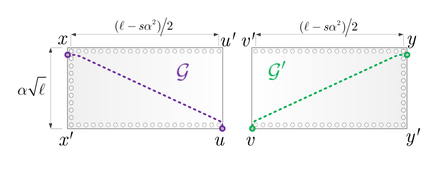
Ψ2\displaystyle\Psi_{2} =πR∗∗​(σx​σy​σu​σv)≥πR∗∗​(σx​σu)​πR∗∗​(σy​σv)=πR∗∗​(σx​σu)2.\displaystyle=\pi_{R^{*}}^{*}(\sigma_{x}\sigma_{y}\sigma_{u}\sigma_{v})\geq\pi_{R^{*}}^{*}(\sigma_{x}\sigma_{u})\pi_{R^{*}}^{*}(\sigma_{y}\sigma_{v})=\pi_{R^{*}}^{*}(\sigma_{x}\sigma_{u})^{2}\,.
Refer to caption
Figure 12. Domain decrease from the rectangle RR to a disjoint union of rectangles separating the two open contours.

Furthermore, by GKS, spin-spin correlations are non-decreasing in the domain so we can clearly confine our domain to the disjoint union of the two rectangles 𝒢=(x,u′,u,x′)\mathcal{G}=(x,u^{\prime},u,x^{\prime}) as shown in Figure 12, and obtain by symmetry that

Ψ2≥X2 where ​X:=π𝒢∗∗​(σx​σu).\Psi_{2}\geq X^{2}\quad\mbox{ where }X:=\pi^{*}_{\mathcal{G}^{*}}(\sigma_{x}\sigma_{u})\,.

To control the value of XX, let zz be the center of the rectangle 𝒢\mathcal{G} and further define 𝒢1=(x,a,b,x′)\mathcal{G}_{1}=(x,a,b,x^{\prime}) and 𝒢2=(a,u′,u,b)\mathcal{G}_{2}=(a,u^{\prime},u,b) to be the left and right halves of 𝒢\mathcal{G}, each of dimensions 14​(ℓ−s​α2)×α​ℓ\tfrac{1}{4}(\ell-s\alpha^{2})\times\alpha\sqrt{\ell}. See Figure 13 for an illustration. The GKS-inequalities (together with a reduction of the domain) yield

π𝒢∗∗​(σx​σu)≥π𝒢1∗∗​(σx​σz)​π𝒢2∗∗​(σu​σz).\pi^{*}_{\mathcal{G}^{*}}(\sigma_{x}\sigma_{u})\geq\pi^{*}_{\mathcal{G}_{1}^{*}}(\sigma_{x}\sigma_{z})\pi^{*}_{\mathcal{G}_{2}^{*}}(\sigma_{u}\sigma_{z})\,.

Another application of  (2.7) gives

X\displaystyle X ≥∑λ⊂𝒢1δ​λ={x,z}q𝒢1∗​(λ)​∑λ⊂𝒢2δ​λ={u,z}q𝒢2∗​(λ)=(∑λ⊂𝒢1δ​λ={x,z}q𝒢1∗​(λ))2,\displaystyle\geq\sum_{\begin{subarray}{c}\lambda\subset\mathcal{G}_{1}\\ \delta\lambda=\{x,z\}\end{subarray}}q_{\mathcal{G}_{1}^{*}}(\lambda)\sum_{\begin{subarray}{c}\lambda\subset\mathcal{G}_{2}\\ \delta\lambda=\{u,z\}\end{subarray}}q_{\mathcal{G}_{2}^{*}}(\lambda)=\bigg(\sum_{\begin{subarray}{c}\lambda\subset\mathcal{G}_{1}\\ \delta\lambda=\{x,z\}\end{subarray}}q_{\mathcal{G}_{1}^{*}}(\lambda)\bigg)^{2}\,,

with the equality due to symmetry. Define S¯\bar{S} to be the infinite half-strip of width 14​(ℓ−s​α2)\frac{1}{4}(\ell-s\alpha^{2}) obtained by extending the South border of 𝒢1\mathcal{G}_{1} (i.e. the edge b​x′bx^{\prime}) to −∞-\infty. Since 𝒢1\mathcal{G}_{1} is a subgraph of S¯\bar{S} it follows from Lemma 2.2 that

X≥X¯2 where X¯:=∑λ⊂𝒢1δ​λ={x,z}qS¯∗​(λ).X\geq\bar{X}^{2}\quad\mbox{ where }\quad\bar{X}:=\sum_{\begin{subarray}{c}\lambda\subset\mathcal{G}_{1}\\ \delta\lambda=\{x,z\}\end{subarray}}q_{\bar{S}^{*}}(\lambda)\,.

We now claim that

X¯Y¯≥1−(ℓ/4)c1​exp⁡(−c2​α2),\frac{\bar{X}}{\bar{Y}}\geq 1-(\ell/4)^{c_{1}}\exp(-c_{2}\alpha^{2})\,, (6.6)

where

Y¯:=∑λ⊂S¯δ​λ={x,z}qS¯∗​(λ).\bar{Y}:=\sum_{\begin{subarray}{c}\lambda\subset\bar{S}\\ \delta\lambda=\{x,z\}\end{subarray}}q_{\bar{S}^{*}}(\lambda)\,.

Indeed, X¯/Y¯\bar{X}/\bar{Y} is precisely the probability that the contour λ⊂S¯n\lambda\subset\bar{S}_{n} whose endpoints are δ​λ={x,z}\delta\lambda=\{x,z\} stays above the horizontal line x′​bx^{\prime}b (the South border of 𝒢1\mathcal{G}_{1}). If z′z^{\prime} is the midpoint of xx and x′x^{\prime} then by monotonicity if we condition all (+)(+) in the rectangle (x,a,z,z′)(x,a,z,z^{\prime}) then this only increases the probability that the contour hits the line x′​bx^{\prime}b. Proposition 4.4 then establishes equation (6.6). Taking c3c_{3} large enough in the statement of Lemma 6.1 we can assume that α\alpha is at least a large constant times log⁡ℓ\sqrt{\log\ell}, in which case (6.6) gives X¯=(1−o⁡(1))​Y¯\bar{X}=(1-o(1))\bar{Y}.

Refer to caption
Figure 13. Comparing the weight of contours from xx to uu to that of contours connecting both points to the center of the rectangle zz.

On the other hand, taking SS to be the strip obtained by extending the North and South boundaries of 𝒢1\mathcal{G}_{1} to ±∞\pm\infty, we can now express Y¯\bar{Y} in terms of

Y:=∑λ⊂Sδ​λ={x,z}qS∗​(λ).Y:=\sum_{\begin{subarray}{c}\lambda\subset S\\ \delta\lambda=\{x,z\}\end{subarray}}q_{S^{*}}(\lambda)\,.

To this end, observe that Y¯/Y\bar{Y}/Y is the probability that the open contour λ\lambda connecting x,zx,z in SS stays below the horizontal line x​axa (the North border of 𝒢1\mathcal{G}_{1}). Therefore, by monotonicity and Theorem 5.1 there exists some c=c⁡(β)c=c(\beta) such that

Y¯Y≥c/ℓ,\frac{\bar{Y}}{Y}\geq c/\ell\,, (6.7)

and on the other hand [17]*Formula (2.22) gives for some cβ>0c_{\beta}>0

Y=cβ+o⁡(1)ℓ​exp⁡(−τβ​(x−z)).Y=\frac{c_{\beta}+o(1)}{\sqrt{\ell}}\exp(-\tau_{\beta}(x-z))\,. (6.8)

Combining (6.6),(6.7) and (6.8) it now follows that

X¯≥c1′​ℓ−c2′​exp⁡(−τβ​(x−z)),\bar{X}\geq c_{1}^{\prime}\ell^{-c_{2}^{\prime}}\exp(-\tau_{\beta}(x-z))\,,

and recalling that Ψ2≥X2≥X¯4\Psi_{2}\geq X^{2}\geq\bar{X}^{4} we deduce that there exists some c′′​(β)>0c^{\prime\prime}(\beta)>0 such that

Ψ2≥c′′​ℓ−c′′​exp⁡(−2​τβ​(x−u)).\Psi_{2}\geq c^{\prime\prime}\ell^{-c^{\prime\prime}}\exp(-2\tau_{\beta}(x-u))\,. (6.9)

To conclude the proof, we combine (6.5), (6.9) and get that

Ψ1Ψ2≤(1/c′′)​ℓc′′​exp⁡(−[ℓ+s​α2]​τβ​(0)+2​τβ​(x−u)).\frac{\Psi_{1}}{\Psi_{2}}\leq(1/c^{\prime\prime})\ell^{c^{\prime\prime}}\exp\left(-\left[\ell+s\alpha^{2}\right]\tau_{\beta}(0)+2\tau_{\beta}(x-u)\right)\,.

Recall that τβ​(θ)\tau_{\beta}(\theta) is an analytic and even function of θ\theta for any β>βc\beta>\beta_{c}, hence in particular there exists some c=c⁡(β)>0c=c(\beta)>0 such that

τβ​(θ)−τβ​(0)≤c​θ2​ for any θ∈ℝ.\tau_{\beta}(\theta)-\tau_{\beta}(0)\leq c\theta^{2}\mbox{ for any $\theta\in\mathbb{R}$.}

Since in our case θ≤arctan⁡(α​ℓℓ/2)≤2​α/ℓ\theta\leq\arctan\big(\frac{\alpha\sqrt{\ell}}{\ell/2}\big)\leq 2\alpha/\sqrt{\ell} it follows that for some c′=c′​(β)>0c^{\prime}=c^{\prime}(\beta)>0

τβ​(x−u)≤τβ​(0)​|x−u|+c′​α2.\tau_{\beta}(x-u)\leq\tau_{\beta}(0)|x-u|+c^{\prime}\alpha^{2}\,.

On the other hand,

ℓ+s​α2−|x−u|=O⁡(s​α2).\ell+s\alpha^{2}-|x-u|=O(s\alpha^{2})\,.

Combining these inequalities completes the proof. ∎

We next wish to show that whenever δ​λ1={x,u},δ​λ2={y,v}\delta\lambda_{1}=\{x,u\}\,,\,\delta\lambda_{2}=\{y,v\} we also have that the corresponding open contours are confined to the RlR_{l} and RrR_{r}, the left and right halves of RR respectively, except with an appropriate exponentially small probability. The complement event we wish to analyze is illustrated in Figure 14.

Refer to caption
Figure 14. Open contours under b.c. (−,+,Δ)(-,+,\Delta) crossing the central column of RR, addressed by the estimate in Lemma 6.2.
Lemma 6.2.

Let R=(x,y,y′,x′)R=(x,y,y^{\prime},x^{\prime}) and Δ\Delta be an interval of length s​α2s\alpha^{2} centered on the South border x′​y′x^{\prime}y^{\prime}. Denote by RlR_{l} and RrR_{r} the left and right halves of RR respectively. For any β>βc\beta>\beta_{c} there exist c5,c6>0c_{5},c_{6}>0 and s0>0s_{0}>0 depending only on β\beta such that if s≥s0s\geq s_{0} then for any ℓ∈ℕ\ell\in\mathbb{N} we have

πRη(λ1⊂Rl,λ2⊂Rr|δλ1={x,u},δλ2={y,v})≥1−ℓc5exp(−c6α2).\pi_{R}^{\eta}\left(\lambda_{1}\subset R_{l}\,,\,\lambda_{2}\subset R_{r}\;\big|\;\delta\lambda_{1}=\{x,u\}\,,\,\delta\lambda_{2}=\{y,v\}\right)\geq 1-\ell^{c_{5}}\exp(-c_{6}\alpha^{2})\,.
Proof.

Let II denote the central column of RR, i.e. II is the vertical line connecting the centers of the North and South boundaries of RR. We aim to bound the probability that the contour connecting xx to uu crosses II, and similarly for the contour connecting yy to vv. By equality (2.8) we can write the former probability as Φ1/Φ2\Phi_{1}/\Phi_{2} where

Φ1:=∑λ¯=(λ1,λ2)δ​λ1={x,u},λ1∩I≠∅δ​λ2={y,v}qR∗​(λ¯),\displaystyle\Phi_{1}:=\sum_{\begin{subarray}{c}\underline{\lambda}=(\lambda_{1},\lambda_{2})\\ \delta\lambda_{1}=\{x,u\}\,,\,\lambda_{1}\cap I\neq\emptyset\\ \delta\lambda_{2}=\{y,v\}\end{subarray}}q_{R^{*}}(\underline{\lambda})\,, Φ2:=∑λ¯=(λ1,λ2)δ​λ¯1={x,u}δ​λ¯2={y,v}qR∗​(λ¯),\displaystyle\Phi_{2}:=\sum_{\begin{subarray}{c}\underline{\lambda}=(\lambda_{1},\lambda_{2})\\ \delta\underline{\lambda}_{1}=\{x,u\}\\ \delta\underline{\lambda}_{2}=\{y,v\}\end{subarray}}q_{R^{*}}(\underline{\lambda})\,,

and a union bound (together with symmetry) gives

πRη(λ1⊂Rl,λ2⊂Rr|δλ1={x,y},δλ2={u,v})≥1−2Φ1Φ2.\pi_{R}^{\eta}\left(\lambda_{1}\subset R_{l}\,,\,\lambda_{2}\subset R_{r}\;\big|\;\delta\lambda_{1}=\{x,y\}\,,\,\delta\lambda_{2}=\{u,v\}\right)\geq 1-2\frac{\Phi_{1}}{\Phi_{2}}\,.

To bound Φ2\Phi_{2} from below we compare it to Ψ1,Ψ2\Psi_{1},\Psi_{2} defined in (6.4). Indeed,

Φ2Ψ2=1−Ψ1Ψ2=1−πRη​(δ​λ1={x,y},δ​λ2={u,v})≥1−ℓc3​exp⁡(−c4​α2),\frac{\Phi_{2}}{\Psi_{2}}=1-\frac{\Psi_{1}}{\Psi_{2}}=1-\pi_{R}^{\eta}(\delta\lambda_{1}=\{x,y\}\,,\,\delta\lambda_{2}=\{u,v\})\geq 1-\ell^{c_{3}}\exp(-c_{4}\alpha^{2})\,,

where the last inequality is precisely the statement of Lemma 6.1. Combining this with the estimate on Ψ2\Psi_{2} given in  (6.9) we conclude that for some absolute c′′>0c^{\prime\prime}>0,

Φ2≥(1−ℓc3​exp⁡(−c4​α2))​c′′​ℓ−c′′​e−τβ​(x−u)−τβ​(y−v)\Phi_{2}\geq\left(1-\ell^{c_{3}}\exp(-c_{4}\alpha^{2})\right)c^{\prime\prime}\ell^{-c^{\prime\prime}}e^{-\tau_{\beta}(x-u)-\tau_{\beta}(y-v)} (6.10)

(we can assume that α\alpha is at least a large constant times log⁡ℓ\sqrt{\log\ell}, otherwise the statement of Lemma 6.2 trivially holds).

Remark.

The estimate given in (6.9) for Ψ2\Psi_{2} in the proof of Lemma 6.1 in fact had an exponent of −2​τβ​(x−u)-2\tau_{\beta}(x-u). The above bound featuring −(τβ​(x−u)+τβ​(y−v))-(\tau_{\beta}(x-u)+\tau_{\beta}(y-v)) in the exponent readily follows from (6.9) by the symmetry between {x,u}\{x,u\} and {y,v}\{y,v\} in the definition of Ψ2\Psi_{2}.

It remains to bound Φ1\Phi_{1}. To this end, for a given contour γ\gamma define 𝒢γ\mathcal{G}_{\gamma} to be the graph with the edge-set R∗∖Δ⁡(γ)R^{*}\setminus\Delta(\gamma), where Δ⁡(γ)\Delta(\gamma) is the edge-boundary of the contour γ\gamma. Crucially, in our case the edge-boundary of γ\gamma is disjoint to the edges of λ1\lambda_{1} since these contours are compatible. Therefore, by Lemma 2.3,

qR∗​(λ,γ)=qR∗​(γ)​q𝒢γ​(λ),q_{R^{*}}(\lambda,\gamma)=q_{R^{*}}(\gamma)q_{\mathcal{G}_{\gamma}}(\lambda)\,,

and plugging this into the definition of Φ1\Phi_{1} we deduce that

Φ1=∑γ:δ​γ={y,v}(qR∗(γ)∑λ:δ​λ={x,u}λ∩I≠∅q𝒢γ(λ)).\Phi_{1}=\sum_{\gamma\,:\,\delta\gamma=\{y,v\}}\bigg(q_{R^{*}}(\gamma)\sum_{\begin{subarray}{c}\lambda\,:\,\delta\lambda=\{x,u\}\\ \lambda\cap I\neq\emptyset\end{subarray}}q_{\mathcal{G}_{\gamma}}(\lambda)\bigg)\,.

The sum over the weights q𝒢γq_{\mathcal{G}_{\gamma}} can be estimated via Corollary 2.5 using a simple union bound (see e.g. [8]*Eq.(3.3) for a similar argument). Indeed,

∑λ:δ​λ={x,u}λ∩I≠∅q𝒢γ(λ)≤∑z∈I∑λ:δ​λ={x,u}z∈λq𝒢γ(λ)≤∑z∈Iπ𝒢γ∗(σxσz)π𝒢γ∗(σuσz).\sum_{\begin{subarray}{c}\lambda\,:\,\delta\lambda=\{x,u\}\\ \lambda\cap I\neq\emptyset\end{subarray}}q_{\mathcal{G}_{\gamma}}(\lambda)\leq\sum_{z\in I}\sum_{\begin{subarray}{c}\lambda:\,\delta\lambda=\{x,u\}\\ z\in\lambda\end{subarray}}q_{\mathcal{G}_{\gamma}}(\lambda)\leq\sum_{z\in I}\pi_{\mathcal{G}_{\gamma}}^{*}\left(\sigma_{x}\,\sigma_{z}\right)\,\pi_{\mathcal{G}_{\gamma}}^{*}\left(\sigma_{u}\,\sigma_{z}\right)\,.

At the same time, we can use (2.7) and then increase the appropriate domains to the infinite-volume lattice to obtain that

∑γ:δ​γ={y,v}qR∗(γ)\displaystyle\sum_{\gamma\,:\,\delta\gamma=\{y,v\}}q_{R^{*}}(\gamma) ≤π∞∗​(σy​σv),\displaystyle\leq\pi^{*}_{\infty}(\sigma_{y}\,\sigma_{v})\,,
∑λ:δ​λ={x,u}λ∩I≠∅q𝒢γ(λ)\displaystyle\sum_{\begin{subarray}{c}\lambda\,:\,\delta\lambda=\{x,u\}\\ \lambda\cap I\neq\emptyset\end{subarray}}q_{\mathcal{G}_{\gamma}}(\lambda) ≤∑z∈Iπ∞∗​(σx​σz)​π∞∗​(σu​σz),\displaystyle\leq\sum_{z\in I}\pi^{*}_{\infty}(\sigma_{x}\,\sigma_{z})\,\pi_{\infty}^{*}(\sigma_{u}\,\sigma_{z})\,,

where here π∞∗\pi_{\infty}^{*} denotes the (unique) Gibbs measure on ℤ2\mathbb{Z}^{2} at β∗\beta^{*}. Altogether,

Φ1\displaystyle\Phi_{1} ≤∑z∈Iπ∞∗​(σx​σz)​π∞∗​(σz​σu)​π∞∗​(σy​σv)\displaystyle\leq\sum_{z\in I}\pi_{\infty}^{*}(\sigma_{x}\,\sigma_{z})\pi_{\infty}^{*}(\sigma_{z}\,\sigma_{u})\pi_{\infty}^{*}(\sigma_{y}\,\sigma_{v})
≤∑z∈Iexp⁡(−τβ​(z−x)−τβ​(z−u)−τβ​(y−v)).\displaystyle\leq\sum_{z\in I}\exp\left(-\tau_{\beta}(z-x)-\tau_{\beta}(z-u)-\tau_{\beta}(y-v)\right)\,.

At the same time, due to the sharp triangle inequality property of the surface tension (Eq. (2.2)), for any β>βc\beta>\beta_{c} there exists some κβ>0\kappa_{\beta}>0 such that for any u,x,zu,x,z

τβ​(z−x)\displaystyle\tau_{\beta}(z-x) +τβ​(u−z)≥τβ​(u−x)+κβ​(|z−x|+|u−z|−|u−x|).\displaystyle+\tau_{\beta}(u-z)\geq\tau_{\beta}(u-x)+\kappa_{\beta}\left(|z-x|+|u-z|-|u-x|\right)\,.

Combining the last two displays implies that

Φ1\displaystyle\Phi_{1} ≤e−τβ​(x−u)−τβ​(y−v)​∑z∈Iexp⁡[−κβ​(|z−x|+|u−z|−|u−x|)].\displaystyle\leq e^{-\tau_{\beta}(x-u)-\tau_{\beta}(y-v)}\sum_{z\in I}\exp\left[-\kappa_{\beta}\left(|z-x|+|u-z|-|u-x|\right)\right]\,. (6.11)

The first term above cancels when combining (6.11),(6.10) and we obtain that for some c′′>0c^{\prime\prime}>0,

Φ1Φ2≤c′′​ℓc′′​∑z∈Iexp⁡[−κβ​(|z−x|+|u−z|−|u−x|)].\frac{\Phi_{1}}{\Phi_{2}}\leq c^{\prime\prime}\ell^{c^{\prime\prime}}\sum_{z\in I}\exp\left[-\kappa_{\beta}\left(|z-x|+|u-z|-|u-x|\right)\right]\,. (6.12)

A straightforward manipulation of the above exponent will now complete the proof: One can easily infer from the triangle-inequality and symmetry that

minz∈I⁡(|z−x|+|u−z|−|u−x|)=|v−x|−|u−x|,\min_{z\in I}\left(|z-x|+|u-z|-|u-x|\right)=|v-x|-|u-x|\,,

and recalling that the dimensions of RR are α​ℓ×ℓ\alpha\sqrt{\ell}\times\ell and |u−v|=s​α2|u-v|=s\alpha^{2}, we have

|v−x|2\displaystyle|v-x|^{2} =14​(ℓ+s​α2)2+α2​ℓ,\displaystyle=\tfrac{1}{4}(\ell+s\alpha^{2})^{2}+\alpha^{2}\ell\,, |u−x|2=14​(ℓ−s​α2)2+α2​ℓ.\displaystyle|u-x|^{2}=\tfrac{1}{4}(\ell-s\alpha^{2})^{2}+\alpha^{2}\ell\,.

Hence, as long as α<(1/s)​ℓ\alpha<(1/s)\sqrt{\ell} (guaranteed by the assumptions of Proposition 4.5) we have |u−x|+|v−x|≤2​ℓ|u-x|+|v-x|\leq 2\ell and

|v−x|−|u−x|=s​α2​ℓ|u−x|+|v−x|≥12​s​α2.|v-x|-|u-x|=\frac{s\alpha^{2}\ell}{|u-x|+|v-x|}\geq\frac{1}{2}s\alpha^{2}\,.

Plugging this in (6.12) while summing over the |I||I| values that zz can assume gives that

Φ1Φ2≤c′′​ℓc′′+1​exp⁡(−(κβ/2)​s​α2)\frac{\Phi_{1}}{\Phi_{2}}\leq c^{\prime\prime}\ell^{c^{\prime\prime}+1}\exp(-(\kappa_{\beta}/2)s\alpha^{2})

(with room to spare), as required. ∎

Acknowledgments

We are very grateful to Yvan Velenik for valuable suggestions on the random-line representation and related equilibrium estimates, as well as for pointing out the novelty of Corollary 5.2. EL and AS are grateful to the Mathematics Department of the University of Roma Tre for hospitality and support. FM and FLT are similarly grateful to the Theory Group of Microsoft Research. FLT acknowledges partial support by ANR grant LHMSHE.

References

  • [1] D. B. Abraham and P. Reed (1974) Phase separation in the two-dimensional ising ferromagnet. Phys. Rev. Lett. 33 (6), pp. 377–379. Cited by: §1.3.
  • [2] K. S. Alexander and N. Yoshida (2001) The spectral gap of the 2-d stochastic ising model with mixed boundary conditions. J. Statist. Phys. 104 (1-2), pp. 89–109. Cited by: §1.3.
  • [3] K. S. Alexander (2001) The spectral gap of the 2-d stochastic ising model with nearly single-spin boundary conditions. J. Statist. Phys. 104 (1-2), pp. 59–87. Cited by: §1.3.
  • [4] A. Bianchi (2008) Glauber dynamics on nonamenable graphs: boundary conditions and mixing time. Electronic Journal of Probability 13, pp. 1980–2012. Cited by: §1.3.
  • [5] T. Bodineau and F. Martinelli (2002) Some new results on the kinetic ising model in a pure phase. J. Statist. Phys. 109 (1-2), pp. 207–235. Cited by: §1.1, §1.3.
  • [6] J. Bricmont, A. El Mellouki, and J. Fröhlich (1982) Random surfaces in statistical mechanics: roughening, rounding, wetting…. J. Statist. Phys. 29, pp. 193–203. Cited by: §5, §5.
  • [7] P. Caputo, F. Martinelli, F. Simenhaus, and F. L. Toninelli “Zero” temperature stochastic 3d ising model and dimer covering fluctuations: a first step towards interface mean curvature motion. (Comm. Pure Appl. Math., to appear). Note: Available at arXiv:1007.3599 (2010) Cited by: §1.1, §1.3.
  • [8] F. Cesi, G. Guadagni, F. Martinelli, and R. H. Schonmann (1996) On the two-dimensional stochastic ising model in the phase coexistence region near the critical point. J. Statist. Phys. 85 (1-2), pp. 55–102. Cited by: §1.2, §1, §6.2.
  • [9] L. Chayes, R. H. Schonmann, and G. Swindle (1995) Lifshitz’ law for the volume of a two-dimensional droplet at zero temperature. J. Statist. Phys. 79 (5-6), pp. 821–831. Cited by: §1.3, §1.
  • [10] R. Dobrushin and O. Hryniv (1997) Fluctuations of the phase boundary in the 22d ising ferromagnet. Comm. Math. Phys. 189 (2), pp. 395–445. Cited by: §1.
  • [11] R. Dobrushin, R. Kotecký, and S. Shlosman (1992) Wulff construction. a global shape from local interaction. Translations of Mathematical Monographs, Vol. 104, American Mathematical Society. Note: Translated from Russian by the authors Cited by: §1, §2.2, §3.1, §3.
  • [12] D. S. Fisher and D. A. Huse (1987) Dynamics of droplet fluctuations in pure and random ising systems. Phys. Rev. B 35 (13), pp. 6841–6846. Cited by: §1.2, §1.
  • [13] L. R. Fontes, R. H. Schonmann, and V. Sidoravicius (2002) Stretched exponential fixation in stochastic ising models at zero temperature. Comm. Math. Phys. 228 (3), pp. 495–518. Cited by: §1.3.
  • [14] C. M. Fortuin, P. W. Kasteleyn, and J. Ginibre (1971) Correlation inequalities on some partially ordered sets. Comm. Math. Phys. 22, pp. 89–103. Cited by: §1.1.
  • [15] G. Gallavotti (1972) The phase separation line in the two-dimensional ising model. Comm. Math. Phys. 27, pp. 103–136. Cited by: §1.3.
  • [16] R. J. Glauber (1963) Time-dependent statistics of the ising model. J. Mathematical Phys. 4, pp. 294–307. Cited by: §1.
  • [17] L. Greenberg and D. Ioffe (2005) On an invariance principle for phase separation lines. Ann. Inst. H. Poincaré Probab. Statist. 41 (5), pp. 871–885. Cited by: §2.3, §6.2, Abstract..
  • [18] R. B. Griffiths (1967) Correlations in ising ferromagnets. iii. a mean-field bound for binary correlations. Comm. Math. Phys. 6 (2), pp. 121–127. Cited by: Lemma 2.1, §6.2.
  • [19] Y. Higuchi (1979) On some limit theorems related to the phase separation line in the two-dimensional ising model. Z. Wahrsch. Verw. Gebiete 50 (3), pp. 287–315. Cited by: §1, Abstract..
  • [20] O. Hryniv (1998) On local behaviour of the phase separation line in the 2D Ising model. Probability Theory and Related Fields 110, pp. 91–107. Cited by: §1, §5, Abstract..
  • [21] D. Ioffe (1994) Large deviations for the 22d ising model: a lower bound without cluster expansions. J. Statist. Phys. 74 (1-2), pp. 411–432. Cited by: §2.2.
  • [22] D. Ioffe (1995) Exact large deviation bounds up to TcT_{c} for the ising model in two dimensions. Probability Theory Related Fields 102 (3), pp. 313–330. Cited by: §2.2.
  • [23] D. G. Kelly and S. Sherman (1968) General griffiths’ inequalities on correlations in ising ferromagnets. J. Math. Phys. 9 (3), pp. 466–484. Cited by: Lemma 2.1, §6.2.
  • [24] D. A. Levin, Y. Peres, and E. Wilmer (2008) Markov chains and mixing times. American Mathematical Society. Cited by: §1.1.
  • [25] I. M. Lifshitz (1962) Kinetics of ordering during second-order phase transitions. Sov. Phys. JETP 15, pp. 939. Cited by: §1.
  • [26] T. M. Liggett (2005) Interacting particle systems. Classics in Mathematics, Springer-Verlag. Note: Reprint of the 1985 original Cited by: §1.1.
  • [27] E. Lubetzky and A. Sly Critical ising on the square lattice mixes in polynomial time. (preprint). Note: Available at arXiv:1001.1613 (2010) Cited by: §1.
  • [28] F. Martinelli and E. Olivieri (1994) Approach to equilibrium of glauber dynamics in the one phase region. i. the attractive case. Comm. Math. Phys. 161 (3), pp. 447–486. Cited by: §1.
  • [29] F. Martinelli and E. Olivieri (1994) Approach to equilibrium of glauber dynamics in the one phase region. ii. the general case. Comm. Math. Phys. 161 (3), pp. 487–514. Cited by: §1.
  • [30] F. Martinelli (1994) On the two-dimensional dynamical ising model in the phase coexistence region. J. Statist. Phys. 76 (5-6), pp. 1179–1246. Cited by: §1.3, §1.
  • [31] F. Martinelli, A. Sinclair, and D. Weitz (2004) Glauber dynamics on trees: boundary conditions and mixing time. Comm. Math. Phys. 250 (2), pp. 301–334. Cited by: §1.3.
  • [32] F. Martinelli and A. Sinclair Mixing time for the solid-on-solid model. pp. 571–580. Cited by: §1.3.
  • [33] F. Martinelli and F. L. Toninelli (2010) On the mixing time of the 22d stochastic ising model with “plus” boundary conditions at low temperature. Comm. Math. Phys. 296 (1), pp. 175–213. Cited by: §1.2, §1.2, §1.2, §1.3, §1, §1, §3.1, §3.1, §3.1, §3.1, §3.1, §3.1, §3.1, Lemma 3.6, §3, §3, §3, §4, §4, §4, Remark, Abstract., Abstract..
  • [34] F. Martinelli (1999) Lectures on glauber dynamics for discrete spin models. pp. 93–191. Cited by: §1.1, §2.1.
  • [35] B. M. McCoy and T. T. Wu (1973) The two-dimensional ising model. Harvard University Press. Cited by: Lemma 2.1, §5, §5.
  • [36] A. T. Ogielski (1987) Dynamics of fluctuations in the ordered phase of kinetic ising models. Phys. Rev. B 36 (13), pp. 7315–7318. Cited by: §1.
  • [37] L. Onsager (1944) Crystal statistics. i. a two-dimensional model with an order-disorder transition. Phys. Rev. (2) 65, pp. 117–149. Cited by: §1.
  • [38] Y. Peres Note: Summary available at http://www.stat.berkeley.edu/˜peres/ubc.pdf Cited by: §3.
  • [39] C.-E. Pfister and Y. Velenik (1997) Large deviations and continuum limit in the 22d ising model. Probab. Theory Related Fields 109 (4), pp. 435–506. Cited by: §1.3, §1, §2.5, Corollary 2.5, Lemma 2.6, §5, §5, §5.
  • [40] C.-E. Pfister and Y. Velenik (1999) Interface, surface tension and reentrant pinning transition in the 22d ising model. Comm. Math. Phys. 204 (2), pp. 269–312. Cited by: §1.3, §1, §2.2, §2.2, §2.5, §2.5, §2.5, Lemma 2.2, Lemma 2.3, Lemma 2.4, §5, §5.
  • [41] C.-E. Pfister (1991) Large deviations and phase separation in the two-dimensional ising model. Helv. Phys. Acta 64 (7), pp. 953–1054. Cited by: §1.3, §2.2.
  • [42] L. Saloff-Coste (1997) Lectures on finite markov chains. pp. 301–413. Cited by: §1.1.
  • [43] S. B. Shlosman (1989) The droplet in the tube: a case of phase transition in the canonical ensemble. Comm. Math. Phys. 125 (1), pp. 81–90. Cited by: §2.2.
  • [44] H. Spohn (1993) Interface motion in models with stochastic dynamics. J. Statist. Phys. 71 (5-6), pp. 1081–1132. Cited by: §1.
  • [45] N. Sugimine (2002) A lower bound on the spectral gap of the 3-dimensional stochastic ising models. J. Math. Kyoto Univ. 42 (4), pp. 751–788 (2003). Cited by: §1.3.
  • [46] L. E. Thomas (1989) Bound on the mass gap for finite volume stochastic ising models at low temperature. Comm. Math. Phys. 126 (1), pp. 1–11. Cited by: §1.3.