Light bending in a Coulombic field
Abstract
The nonlinear Euler-Heisenberg interaction bends light toward an electric charge. The bending angle and trajectory of light in a Coulombic field are computed in geometric optics.
pacs
12.20.Fv,07.60.Ly,41.20.JbThe light bending by a massive object is one of the prominent features of the general relativity and is a useful tool in astrophysics through the gravitational lensing. Though not directly related in physics, a question may be raised whether there is an electrodynamic version of the bending: that is, whether an electric charge can bend light toward, or outward of it. Though it may most probably be very difficult to observe the effect we, nevertheless, think it is interesting to address the question.
At classical level the linearity of the electrodynamics precludes bending of light, and therefore any bending must involve a nonlinear interaction from quantum corrections. The Euler-Heisenberg interaction that arises from the box diagram in quantum electrodynamics can provide such a nonlinear interaction.
In this note we show that an electric charge bends light toward it through the Euler-Heisenberg interaction, and compute the bending angle and trajectory of light in a Coulombic field. The bending of light by Euler-Heisenberg interaction is not new and has been investigated by several authors, particularly on astronomical objects. For instance, Denisov, et al. [1] studied light bending in the dipole magnetic field of a neutron star and De Lorenci, et al. [2] studied the light bending by a charged black hole. But none of the studies specifically addresses our question above, and in addition we develop a simple geometric way of computing the bending angle and trajectory based on the Snell’s law.
The box diagram of quantum electrodynamics gives rise to a low energy effective Lagrangian of Euler-Heisenberg [3, 4]
| (1) |
In the presence of a background electric field the nonlinear interaction modifies the dispersion relation for the electromagnetic wave and results in a modified speed of light that reads [5, 6, 7, 11, 8, 9, 10]
| (2) |
where denotes the unit vector in the direction of propagation. There is birefringence effect of the light speed depending on the photon polarization; The constant is either 14 for the normal mode or 8 for the parallel mode, where the photon polarization is, respectively, perpendicular to or parallel to the plane spanned by and . Because the speed of light depends on the field strength the light bends in presence of a nonuniform field. The bending can be studied in geometric optics by noting that the index of refraction of the background field is given in leading order by
| (3) |
The infinitesimal bending of photon trajectory over can be obtained from the Snell’s law as
| (4) | |||||
where denotes the angle between and (see Fig.1).
For a Coulombic field of charge
| (5) |
and for a photon trajectory on the - plane the refractive index can be written as
| (6) |
Noticing that in (4) can be as well thought as the change in angle between and the -axis the equation for photon trajectory can be easily derived as
| (7) |
where , respectively, denotes the first two components of .
Now for an incoming photon with impact parameter the initial condition reads
| (8) |
and the trajectory equation (7) becomes to the leading order
| (9) |
with at leading order given by
| (10) |
The equation (9) can be easily integrated by putting in for leading order solution to obtain
| (11) |
where
| (12) |
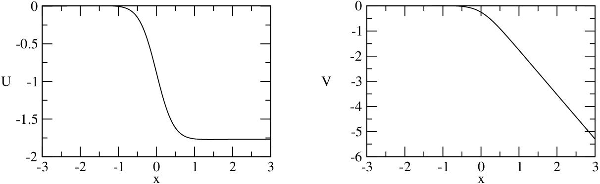
and , and denotes the Compton length of the electron. The plots of the profile functions and for the bending angle and the trajectory show the bending occurs mostly over the region of , and is attractive toward the charge (see Fig.2).
The total bending angle is given by and reads
| (13) |
Let us now briefly comment on the experimental implication of the bending in the Coulombic field by a nucleus of charge . For a nucleus of large the effect of the bending by the strong electric field may be dominant over the perturbative quantum electrodynamics backgrounds such as the Compton scattering. To see this we may compare the cross section of the bending to that of the Compton scattering. Using the classical theory of scattering [12] and putting in (13) we get the cross section at small
| (14) | |||||
which is characterized by the Compton length of the electron (Note that ). Interestingly, the dependence of the cross section on is nonanalytic. Its origin is dimensional; The only dimensional parameter in the Lagrangian (1) is the coefficient () of the Euler-Heisenberg term and because the bending of light is achromatic the cross section must be proportional to the square root of the coefficient. This is why the cross section is proportional to , with the one extra power of coming from the Coulombic field.
Now compare the result to the cross section for Compton scattering that is set by the much smaller nucleus Compton length , which shows the bending effect can easily dominate the Compton scattering, hence may be observable. Nevertheless, the observation may require extreme precision. The bending angle (13) is valid provided the effective Lagrangian of Euler-Heisenberg as well as the geometric optics of the light ray are applicable. The first requires the wavelength of the photon be larger than the electron Compton length, and for the geometric optics applicable the photon in the ray must do multiple scattering via the box diagram in the Coulombic background; This requires the impact parameter , over which distance the bending occurs mostly, be larger than both the electron Compton length and the photon wavelength. Thus is required for the bending angle (13) to be valid. This condition now demands the bending angle be very small. As an example, for we get the bending angle radian for an x-ray of wavelength .
Acknowledgements.
We are grateful to M. Park for useful discussions.References
- [1] V. I. Denisov, I. P. Denisova, and S. I. Svertilov, Dokl. Phys. 46, 705 (2001); Dokl. Akad. Nauk. Ser. Fiz. 380, 435 (2001).
- [2] V. A. De Lorenci, N. Figueiredo, H. H. Fliche, and M. Novello, Astron. Astrophys. 369, 690 (2001), eprint astro-ph/0102296.
- [3] W. Heisenberg and H. Euler, Z. Phys. 98, 714 (1936), eprint physics/0605038.
- [4] J. S. Schwinger, Phys. Rev. 82, 664 (1951).
- [5] Z. Bialynicka-Birula and I. Bialynicki-Birula, Phys. Rev. D2, 2341 (1970).
- [6] S. L. Adler, Annals Phys. 67, 599 (1971).
- [7] J. S. Heyl and L. Hernquist, J. Phys. A30, 6485 (1997), eprint hep-ph/9705367.
- [8] H. Gies (2000), eprint hep-ph/0010287.
- [9] V. A. De Lorenci, R. Klippert, M. Novello, and J. M. Salim, Phys. Lett. B482, 134 (2000), eprint gr-qc/0005049.
- [10] D. Boer and J.-W. Van Holten (2002), eprint hep-ph/0204207.
- [11] W. Dittrich and H. Gies (1998), eprint hep-ph/9806417.
- [12] H. Goldstein, Classical Mechanics (2ed. Addison-Wesley, Amsterdam) (1980).