Universal Hyperbolic Geometry II: A pictorial overview

This paper introduces hyperbolic geometry using only elementary mathematics, without any analysis, and in particular without transcendental functions. Classical hyperbolic geometry, (see for example [6], [7], [8], [9], [10], [11], [15], [17], [23]), is usually an advanced topic studied in the senior years of a university mathematics program, often built up from a foundation of differential geometry. In recent years, a new, simpler and completely algebraic understanding of this subject has emerged, building on the ideas of rational trigonometry ([18] and [19]). This approach is called universal hyperbolic geometry, because it extends the theory to more general settings, namely to arbitrary fields (usually avoiding characteristic two), and because it generalizes to other quadratic forms (see [21]).

The basic reference is Universal Hyperbolic Geometry I: Trigonometry ([22]), which contains accurate definitions, many formulas and complete proofs, but no diagrams. This paper complements that one, providing a pictorial introduction to the subject with a minimum of formulas and no proofs, essentially relying only on planar projective geometry. The reader is encouraged to verify theorems by making explicit constructions and measurements; aside from a single base (null) circle, with only a ruler one can check most of the assertions of this paper in special cases. Alternatively a modern geometry program such as The Geometer’s Sketchpad, C.A.R., Cabri, GeoAlgebra or Cinderella illustrates the subject with a little effort.

Our approach extends the classical Cayley Beltrami Klein, or projective, model of hyperbolic geometry, whose underlying space is the interior of a disk, with lines being straight line segments. In our formulation we consider also the boundary of the disk, which we call the null circle, also points outside the disk, and also points at infinity. The lines are now complete lines in the sense of projective geometry, not segments, and include also null lines which are tangent to the null circle, and lines which do not meet the null circle, including the line at infinity. This orientation is familiar to classical geometers (see for example [2], [3], [4], [5], [14]), but it is not well-known to students because of the current dominance of the differential geometric point of view. A novel aspect of this paper is that we introduce our metrical concepts—quadrance, spread and quadrea—purely in projective terms. It means that only high school algebra suffices to set up the subject and make computations. The proofs however rely generally on computer calculations involving polynomial or rational function identities; some may be found in ([22]), others will appear elsewhere.

Many of the results are illustrated with two diagrams, one illustrating the situation in the classical setting using interior points of the null circle, and another with more general points. The fundamental metrical notions of quadrance between points and spread between lines are undefined when null points or null lines are involved, but most theorems involving them apply equally to points and lines interior or exterior of the null circle. The reader should be aware that in more advanced work the distinction between these two types of points and lines also becomes significant. Instead of area of hyperbolic triangles, we work with a rational analog called quadrea.

With this algebraic approach we can develop geometry over the rational numbers—in my view, always the most important field. The natural connections between geometry and number theory are then not suppressed, but enrich both subjects. Later in the series we will also illustrate hyperbolic geometry over finite fields, in the direction of [1] and [16], where counting becomes important.

Hyperbolic geometry may be visualized as the geometry of the projective plane, augmented by a distinguished circle $c$ (in fact a more general conic may also be used). Since projective geometry is not these days as familiar as it was in former times, we begin by reviewing some of the basic notions. The starting point is the affine plane—familiar from Euclidean geometry and Cartesian coordinate geometry—containing the usual points $\left[x,y\right]$ and (straight) lines with equations $ax+by=c$. The affine plane is augmented by introducing a new point for every family of parallel lines. In this introductory section we use parallel in the usual sense of Euclidean geometry, so that the lines with equations $a_{1}x+b_{1}y=c_{1}$ and $a_{2}x+b_{2}y=c_{2}$ are parallel precisely when $a_{1}b_{2}-a_{2}b_{1}=0.$ Later on we will see that there is a different, hyperbolic meaning of ‘parallel’ (which is different from the usage in classical hyperbolic geometry!) The new point, one for each family of parallel lines, is a ‘point at infinity’. We also introduce one new line, the ‘line at infinity’, which passes through every point at infinity.

Algebraically the projective plane may be defined without reference to the Euclidean plane, with points specified by homogeneous coordinates, or proportions, of the form $\left[x:y:z\right]$. Points $\left[x:y:1\right]$ correspond to the affine plane, and points at infinity are of the form $\left[x:y:0\right]$. The lines also are specified by homogeneous coordinates, now of the form $\left(a:b:c\right)$, with the pairing between the point $\left[x:y:z\right]$ and the line $\left(a:b:c\right)$ given by

This particular relation is the characterizing equation for hyperbolic geometry; for spherical/elliptic geometry a different convention between points and lines is used, where the line $\left\langle a:b:c\right\rangle$ passes through the point $\left[x:y:z\right]$ precisely when $ax+by+cz=0.$ Note that we use round brackets for lines in hyperbolic geometry.

We will visualize the projective plane as an extension of the affine plane, with the usual property that any two distinct points $a$ and $b$ determine exactly one line which passes through them both, called the join of $a$ and $b,$ and denoted by $ab,$ and with the new property that any two lines $L$ and $M$ determine exactly one point which lies on them both, called the meet of $L$ and $K,$ and denoted by $LM.$

In projective geometry, the notion of parallel lines disappears, since now any two lines meet. Familiar measurements, such as distance and angle, are also absent. It is really the geometry of the straightedge.

Despite its historical importance, intrinsic beauty and simplicity, projective geometry is these days sadly neglected in the school and university curriculum. Perhaps the wider realization that it actually underpins hyperbolic geometry will lead to a renaissance of the subject! Most readers will know the two basic theorems in the subject, which are illustrated in Figure 1.

Pappus’ theorem asserts that if $a_{1}$, $a_{2}$ and $a_{3}$ are collinear, and $b_{1},b_{2}$ and $b_{3}$ are collinear, then $x_{1}\equiv\left(a_{2}b_{3}\right)\left(a_{3}b_{2}\right)$, $x_{2}\equiv\left(a_{3}b_{1}\right)\left(a_{1}b_{3}\right)$ and $x_{3}\equiv\left(a_{1}b_{2}\right)\left(a_{2}b_{1}\right)$ are collinear. Desargues’ theorem asserts that if $a_{1}b_{1}$, $a_{2}b_{2}$ and $a_{3}b_{3}$ are concurrent, then $x_{1}\equiv\left(a_{2}a_{3}\right)\left(b_{2}b_{3}\right)$, $x_{2}\equiv\left(a_{3}a_{1}\right)\left(b_{3}b_{1}\right)$ and $x_{3}\equiv\left(a_{1}a_{2}\right)\left(b_{1}b_{2}\right)$ are collinear. This is often stated in the form that if two triangles are perspective from a point, then they are also perspective from a line.

A further important notion concerns four collinear points $a,b,c$ and $d$ on a line $L,$ in any order. Suppose we choose affine coordinates on $L$ so that the coordinates of $a,b,c$ and $d$ are respectively $x,y,z$ and $w.$ Then the cross-ratio is defined to be the extended number (possibly $\infty$) given by the ratio of ratios:

This is independent of the choice of affine coordinates on $L$.

Moreover it is also projectively invariant, meaning that if $a_{1},b_{1},c_{1}$ and $d_{1}$ are also collinear points on a line $L_{1}$ which are perspective to $a,b,c$ and $d$ from some point $p,$ as in Figure 2, then $\left(a,b:c,d\right)=\left(a_{1},b_{1}:c_{1},d_{1}\right)$.

The cross ratio is the most important invariant in projective geometry, and will be the basis of quadrance between points and spread between lines, but we give also analytic expressions for these quantities in homogeneous coordinates; both are rational functions of the inputs. The actual values assumed by the cross-ratio depend ultimately on the field over which our geometry is based, which is in principle quite arbitrary. To start it helps to restrict our attention to the rational numbers, invariably the most natural, familiar and important field. So we will adopt a scientific approach, identifying our sheet of paper with (part of) the rational number plane.

Here are a few more basic definitions. A side $\overline{a_{1}a_{2}}=\left\{a_{1},a_{2}\right\}$ is a set of two points. A vertex $\overline{L_{1}L_{2}}=\left\{L_{1},L_{2}\right\}$ is a set of two lines. A couple $\overline{aL}=\left\{a,L\right\}$ is a set consisting of a point $a$ and a line $L$. A triangle $\overline{a_{1}a_{2}a_{3}}=\left\{a_{1},a_{2},a_{3}\right\}$ is a set of three points which are not collinear. A trilateral $\overline{L_{1}L_{2}L_{3}}=\left\{L_{1},L_{2},L_{3}\right\}$ is a set of three lines which are not concurrent. Every triangle $\overline{a_{1}a_{2}a_{3}}$ has three sides, namely $\overline{a_{1}a_{2}},$ $\overline{a_{2}a_{3}}$ and $\overline{a_{1}a_{3}}$, and similarly any trilateral $\overline{L_{1}L_{2}L_{3}}$ has three vertices, namely $\overline{L_{1}L_{2}},$ $\overline{L_{2}L_{3}}$ and $\overline{L_{1}L_{3}}.$

Since the points of a triangle and the lines of a trilateral are distinct, any triangle $\overline{a_{1}a_{2}a_{3}}$ determines an associated trilateral $\overline{L_{1}L_{2}L_{3}}$ where $L_{1}\equiv a_{2}a_{3},$ $L_{2}\equiv a_{1}a_{3}$ and $L_{3}\equiv a_{1}a_{2}.$ Conversely any trilateral $\overline{L_{1}L_{2}L_{3}}$ determines an associated triangle $\overline{a_{1}a_{2}a_{3}}$ where $a_{1}\equiv L_{2}L_{3},$ $a_{2}\equiv L_{1}L_{3}$ and $a_{3}\equiv L_{1}L_{2}.$

We are now ready to introduce the hyperbolic plane, which is just the projective plane which we have just been describing, augmented by a distinguished Euclidean circle $c$ in this plane, called the null circle, which appears in our diagrams always in blue. The points lying on $c$ have a distinguished role, and are called null points. The lines tangent to $c$ have a distinguished role, and are called null lines.

All other points and lines, including the points at infinity and the line at infinity, are for the purposes of elementary universal hyperbolic geometry treated in a non-preferential manner. In particular we do not restrict our attention to only interior points lying inside the circle $c$; this is a big difference with classical hyperbolic geometry; exterior points lying outside the circle are equally important. Similarly we do not restrict our attention to only interior lines which meet $c$ in two points; exterior lines which do not meet $c$ are equally important. Note also that these notions can be defined purely projectively once the null circle $c$ has been specified: interior points do not lie on null lines, while exterior points do, and interior lines pass through null points, while exterior lines do not.

For those who prefer to work with coordinates, we may choose our circle to have homogeneous equation $x^{2}+y^{2}-z^{2}=0,$ or in the plane $z=1$ with coordinates $X\equiv x/z$ and $Y\equiv y/z,$ simply the unit circle $X^{2}+Y^{2}=1.$

The presence of the distinguished null circle $c$ has as its main consequence a complete duality between points and lines of the projective plane, in the sense that every point $a$ has associated to it a particular line $a^{\bot}$ and conversely. This duality is one of the ways in which universal hyperbolic geometry is very different from classical hyperbolic geometry, and it arises from a standard construction in projective geometry involving the distinguished null circle $c$—the notion of polarity. How polarity defines duality is central to the subject.

To define the polar of a point $a$ with respect to the null circle $c,$ draw any two lines through $a$ which each both pass through $c$ in two distinct points, say $\alpha,\beta$ and $\gamma,\delta$ respectively; this is always possible. Now here is a beautiful fact from projective geometry: if $d$ and $e$ are the other two diagonal points of the quadrilateral $\alpha\beta\gamma\delta,$ then the line $de$ does not depend on the two chosen lines through $a,$ but only on $a$ itself. So we say that $de=A\equiv a^{\bot}$ is the dual line of the point $a$, and conversely $a=A^{\bot}$ is the dual point of the line $A.$

The picture is as in Figure 3, showing two different possible configurations for which the above prescriptions both hold. In case $a$ is external to the circle, it is also possible to construct $A\equiv a^{\bot}$ from the tangents to the null circle $c$ passing through $a$ as in Figure 4, but this does not work for an interior point such as $b.$

The construction shows that there is in fact a symmetry between the initial point $a$ and the diagonal points $d$ and $e,$ so that if we started with the point $d,$ its dual would be the line $ae,$ and if we started with the point $e,$ its dual would be the point $ad.$ So this shows another fundamental fact: if $d$ lies on the dual $a^{\perp}$ of the point $a,$ then $a$ lies on the dual $d^{\perp}$ of the point $d.$

So to invert the construction, given a line $A,$ choose two points $d$ and $e$ on it, find the dual lines $d^{\perp}$ and $e^{\perp},$ and define $a\equiv A^{\perp}=d^{\perp}e^{\perp}.$ It is at this point that we need the projective plane, with its points and line at infinity, for if $d^{\perp}$ and $e^{\perp}$ were Euclidean parallel, then $d^{\perp}e^{\perp}$ would be a point at infinity. This situation occurs if we take our line $A$ to be a diameter of the null circle $c,$ in the sense of Euclidean geometry.

What happens when the point $a$ is null? In that case the quadrilateral in the above construction degenerates, and the polar line $a^{\perp}$ is the null line tangent to the null circle at $a.$ So every null line is dual to the unique null point which lies on it, as shown also in Figure 4.

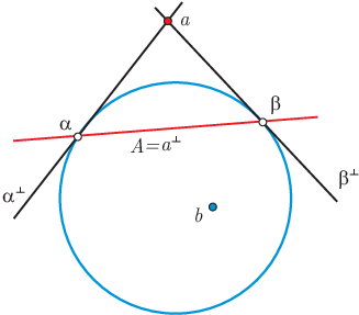
The duality between points and lines is surprisingly simple to describe in terms of homogeneous coordinates. The pole of the point $a\equiv\left[x:y:z\right]$ is just the line $a^{\perp}\equiv\left(x:y:z\right)$, so duality amounts to simply changing from one kind of brackets to the other! This explains why we chose the hyperbolic form of the pairing (1).

In the previous section we saw that every triangle $\overline{a_{1}a_{2}a_{3}}$ has an associated trilateral $\overline{L_{1}L_{2}L_{3}}$ and conversely. Now we see that there is another natural trilateral associated to $\overline{a_{1}a_{2}a_{3}},$ namely the dual trilateral $\overline{a_{1}^{\bot}a_{2}^{\bot}a_{3}^{\bot}}.$ Conversely to any trilateral $\overline{L_{1}L_{2}L_{3}}$ there is associated the dual triangle $\overline{L_{1}^{\bot}L_{2}^{\bot}L_{3}^{\bot}}$.

We also say that a couple $\overline{aL}$ is dual precisely when $a$ and $L$ are dual, and is otherwise non-dual.

So to summarize: in (planar) universal hyperbolic geometry, duality implies that points and lines are treated completely symmetrically. This is a significant departure both from Euclidean geometry and from classical hyperbolic geometry—in both of those theories, points and lines play quite different roles. In universal hyperbolic geometry, the above duality principle implies that every theorem can be dualized to create a (possibly) new theorem. We will state many theorems together with their duals, but to keep the length of this paper reasonable we will not extend this to all the theorems; the reader is encouraged to find statements and draw pictures of the dual results in these other cases.

The notions of perpendicular and parallel differ dramatically between Euclidean and hyperbolic geometries. In the affine geometry on which Euclidean geometry is based, the notion of parallel lines is fundamental, while perpendicular lines are determined by a quadratic form. In hyperbolic geometry, the situation is reversed—perpendicularity is more fundamental, and in fact parallelism is defined in terms of it!

Another novel feature is that perpendicularity applies not only to lines, but also to points. This is a consequence of the fundamental duality we have already established between points and lines.

Perpendicularity in the hyperbolic setting is easy to introduce once we have duality. We say that a point $b$ is perpendicular to a point $a$ precisely when $b$ lies on the dual line $a^{\perp}$ of $a.$ This is equivalent to $a$ lying on the dual line $b^{\perp}$ of $b,$ so the relation is symmetric, and we write

Dually a line $L$ is perpendicular to a line $M$ precisely when $L$ passes through the dual point $M^{\perp}$ of $M.$ This is equivalent to $M$ passing through the dual point $L^{\perp}$ of $L,$ and we write

Figure 6 shows our pictorial conventions for perpendicularity: the line $A\$is dual to the point $a$, so points $b,c$ and $d$ lying on $A$ are perpendicular to $a,$ and this is recorded by a small (right) corner placed on the join of the perpendicular points, and between them. Also the lines $K,L$ and $M$ pass through $a,$ so are perpendicular to $A,$ and this is recorded as usual by a small parallelogram at the meet of the perpendicular lines.

Our first theorem records two basic facts that are obvious from the definitions so far.

We call $N$ the altitude line to $L$ through $a,$ and $n$ the altitude point to $a$ on $L.$ In case $a$ and $L$ are dual, any line through $a$ is perpendicular to $L,$ and any point lying on $L$ is perpendicular to $a.$ While the former idea is familiar, the latter is not. Figure 7 shows that if we restrict ourselves to the inside of the null circle, altitude points are invisible, so it is no surprise that the concept is missing from classical hyperbolic geometry. Remember that we are obliged to respect the balance which duality provides us!

If a triangle $\overline{a_{1}a_{2}a_{3}}$ has say $a_{1}$ dual to $a_{2}a_{3},$ then any line through $a_{1}$ will be perpendicular to the opposite line $a_{2}a_{3},$ and we say the triangle is dual. A triangle is non-dual precisely when each of its points is not dual to the opposite line. Similar definitions apply to trilaterals.

Somewhat surprisingly, the next result is not true in classical hyperbolic geometry—a very conspicuous absence that too often goes unmentioned in books on the subject! The reason is that the orthocenter of a triangle of interior points might well be an exterior point, as the left diagram in Figure 8 shows. The absence of a distinguished orthocenter partially explains why the study of triangles in classical hyperbolic geometry is relatively undeveloped. With universal hyperbolic geometry, triangle geometry enters a rich new phase.

Figure 8 shows a triangle $\overline{a_{1}a_{2}a_{3}}$, its dual trilateral with associated triangle $\overline{l_{1}l_{2}l_{3}},$ and the corresponding orthocenter $o$ and ortholine $O.$

In modern treatments of hyperbolic geometry, points at infinity have a somewhat ambiguous role, and what we call null lines are rarely discussed, because they are essentially invisible in the Beltrami Poincaré models built from differential geometry. However earlier generations of classical geometers were well aware of them (see for example [14]).

In universal hyperbolic geometry null points and null lines play a particularly interesting and important role. Here is a first example, whose name comes from the definition that a triangle is triply nil precisely when each of its points is null.

Figure 9 shows that the Triply nil altitudes theorem may be recast in projective terms: if $l_{1},l_{2}$ and $l_{3}$ are the poles of the lines of the triangle $\overline{\alpha_{1}\alpha_{2}\alpha_{3}}$ with respect to the conic $c,$ then the points $\left(\alpha_{1}\alpha_{3}\right)\left(bl_{1}\right)=\left(bl_{2}\right)^{\bot},$ $\left(\alpha_{2}\alpha_{3}\right)\left(bl_{2}\right)=\left(bl_{1}\right)^{\bot}$ and $l_{3}$ are collinear.

In keeping with triangles and trilaterals, a (cyclic) set of four points is called a quadrangle, and a (cyclic) set of four lines a quadrilateral. The next result restates some facts that we already know about polarity of cyclic quadrilaterals in terms of perpendicularity.

In classical hyperbolic geometry the null points $\alpha_{1},\alpha_{2},\alpha_{3}$ and $\alpha_{4}$ would be considered to be ‘at infinity’, while the external diagonal points $f$ and $g$ in Figure 10 would be invisible. Let us repeat: for us internal and external points are equally interesting.

Points and lines are the basic objects in planar hyperbolic geometry. Given one point $a,$ we may construct its dual line $A\equiv a^{\perp},$ and conversely given a line $A$ we may construct its dual point $a\equiv A^{\perp}.$ After that, there is in general nothing more to construct. For two objects, namely couples, sides and vertices, the situation is considerably more interesting, and gives us a chance to introduce some important additional concepts.

Given a non-dual couple $\overline{aL}$ we know we can construct the dual line $A\equiv a^{\perp}$ and the dual point $l\equiv L^{\perp},$ and the altitude line $N$ and the altitude point $n.$ Now we introduce another major point of departure from classical hyperbolic geometry, which provides an ironic twist to the oft-repeated history of hyperbolic geometry as a development arising from Euclid’s Parallel Postulate.

The line $P$ is the parallel line of the couple $\overline{aL},$ and the point $p$ is the parallel point of the couple $\overline{aL}$. These are shown in Figure 11. We may also refer to $P$ as the parallel line to the line $L$ through $a.$ This is how we will henceforth use the term parallel in universal hyperbolic geometry—we do not say that two lines are parallel.

The point $b$ is the base point of the couple $\overline{aL},$ and the line $B$ is the base line of the couple $\overline{aL}.$ These are shown in Figure 12.

There are also constructions for sides and vertices, and in fact the complete pictures associated with the general couple, side and vertex are essentially the same, but with different objects playing different roles.

Figure 13 shows the constructions possible if we start with a side $\overline{a_{1}a_{2}}.$ Note that in this example one of these points is internal and one is external. A bit more terminology: we say that the side $\overline{a_{1}a_{2}}$ is null precisely when $a_{1}a_{2}$ is a null line, and nil precisely when at least one of $a_{1}$, $a_{2}$ is a null point. The vertex $\overline{L_{1}L_{2}}$ is null precisely when $L_{1}L_{2}$ is a null point, and nil precisely when at least one of $L_{1}$, $L_{2}$ is a null line.

The points $b_{1}$ and $b_{2}$ are the conjugate points of the side $\overline{a_{1}a_{2}}.$ The duals of these points are the lines $B_{1}\equiv a_{1}\left(a_{1}a_{2}\right)^{\bot}$ and $B_{2}\equiv a_{2}\left(a_{1}a_{2}\right)^{\bot}$, which are the conjugate lines of the side $\overline{a_{1}a_{2}}.$ These relations are involutory: if the side $\overline{b_{1}b_{2}}$ is conjugate to the side $\overline{a_{1}a_{2}},$ then $\overline{a_{1}a_{2}}$ is also conjugate to $\overline{b_{1}b_{2}}.$

The same picture can also be reinterpreted by starting with a vertex.

The lines $B_{1}$ and $B_{2}$ are the conjugate lines of the vertex $\overline{A_{1}A_{2}}.$ The duals of these lines are the points $b_{1}\equiv A_{1}\left(A_{1}A_{2}\right)^{\bot}$ and $b_{2}\equiv A_{2}\left(A_{1}A_{2}\right)^{\bot}$, which are the conjugate points of the vertex $\overline{A_{1}A_{2}}.$ This relation is also involutory: if the vertex $\overline{B_{1}B_{2}}$ is conjugate to the vertex $\overline{A_{1}A_{2}},$ then $\overline{A_{1}A_{2}}$ is also conjugate to $\overline{B_{1}B_{2}}.$ This is shown also in Figure 14, which is essentially the same as Figures 12 and 13.

Furthermore the exact same configuration results if we had started with one of the sides $\overline{a_{1}b_{2}},$ or $\overline{a_{2}b_{1}},$ or $\overline{b_{1}b_{2}},$ or with one of the vertices $\overline{A_{1}B_{2}},$ or $\overline{A_{2}B_{1}},$ or $\overline{B_{1}B_{2}}.$ However if we had started with a right side, meaning that the two points are perpendicular, such as $\overline{a_{1}b_{1}},$ then we would obtain $L=a_{1}b_{1}$ and its dual point $l.$ But then the conjugate side of $\overline{a_{1}b_{1}}$ would coincide with $\overline{a_{1}b_{1}},$ and similarly the conjugate vertex of a right vertex such as $\overline{A_{1}B_{1}}$ would coincide with $\overline{A_{1}B_{1}}.$

The basic symmetries of hyperbolic geometry are reflections, but they have a somewhat different character from Euclidean reflections. Hyperbolic reflections send points to points and lines to lines, preserving incidence, in other words they are projective transformations. There are two seemingly different notions, the reflection $\sigma_{a}$ in a (non-null) point $a$, and the reflection $\sigma_{L}$ in a (non-null) line $L$. It is an important fact that these two notions end up agreeing, in the sense that

when $A=a^{\bot}.$

The transformation $\sigma_{a}$ is defined first by its action on null points, and then by its action on more general points and lines.

For a non-null point $a,$ the reflection $\sigma_{a}$ sends a null point $\alpha$ to the other null point $\alpha^{\prime}$ on the line $\alpha a.$ We write

In case $a\alpha$ is a null line, in other words a tangent to the null circle $c,$ then $\alpha^{\prime}\equiv\alpha.$ Note that if $a$ was itself a null point, then this definition would yield a transformation that would send every null point to $a,$ which will not be a symmetry in the sense we wish. However such transformations can still be useful.

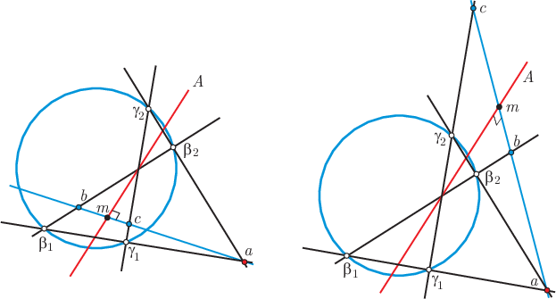
Once the action of a projective transformation on null points is known, it is determined on all points and lines, first of all on lines through two null points, and then on an arbitrary point by means of two such lines passing through it, and then on arbitrary lines. Figure 15 shows the reflection $\sigma_{a}$ and its action on a point $b$ to get $c\equiv b\sigma_{a}.$ First find a line through $b$ meeting the null circle at points $\beta_{1}$ and $\beta_{2}$, then construct $\gamma_{1}\equiv\beta_{1}\sigma_{a}$ and $\gamma_{1}\equiv\beta_{1}\sigma_{a},$ and then set

For the reflection $\sigma_{L}$ in a line $L$, the idea is dual to the above. It is defined first by its action on null lines, and then by its action on more general points and lines. For a non-null line $L,$ the reflection $\sigma_{L}$ sends a null line $\Pi$ to the other null line $\Pi^{\prime}$ passing through the point $L\Pi$. We write

In case $L\Pi$ is a null point, $\Pi^{\prime}\equiv\Pi.$

Once the action of a projective transformation on null lines is known, it is determined on all points and lines, since it is first of all determined on points lying on two null lines, and then on an arbitrary line by means of two such points lying on it, and then on arbitrary points.

Of course there is also a linear algebra/matrix approach to defining reflections. If $a=\left[u:v:w\right]$ then the action of $\sigma_{a}=\sigma_{a^{\perp}}$ on a point $b\equiv\left[x:y:z\right]$ is given by the projective matrix product

where the entries are only determined up to a scalar. The move to three dimensions simplifies the discussion.

The notion of the midpoint of a side can be defined once we have the notion of a reflection. It also has a metrical formulation in terms of quadrance, which we have not yet introduced. There are three other closely related concepts, that of midline, biline and bipoint. Midpoints and midlines refer to sides, while bilines and bipoints refer to vertices. The existence of these objects reduces to questions in number theory—-whether or not certain quadratic equations have solutions.

If $c=b\sigma_{d}$ then we say $d$ is a midpoint of the side $\overline{bc}.$ In this case the point $e\equiv d^{\bot}\left(bc\right)$ is also a midpoint of $\overline{bc}$, and the two midpoints $d$ and $e$ of $\overline{bc}$ are perpendicular. The dual line $D\equiv d^{\bot}$ is a midline of $\overline{bc},$ meaning that it meets $bc$ perpendicularly in a midpoint, namely $e$. The reflection $\sigma_{D}$ in $D$ of $b$ is also $c.$ Similarly the dual line $E\equiv e^{\bot}$ is also a midline of $\overline{bc}.$ In Euclidean geometry midlines are called perpendicular bisectors. In hyperbolic geometry there are generally either zero or two midpoints between any two points, and so also zero or two midlines.

Figure 16 shows the midpoints $m$ and midlines $M$ of a side $\overline{bc}.$

Figure 17 shows how to construct the midpoints and midlines of the side $\overline{bc}$ when such exist. For the midpoints of $\overline{bc}$ we first join $b$ and $c$ to the point $a\equiv\left(bc\right)^{\bot}$ to form lines $M$ and $N.$ If these are both interior lines, then their meets with the null circle give a completely nil quadrangle one of whose diagonal points is $a,$ and the other two diagonal points $d$ and $e$ lie on $bc$ and are the required midpoints. The duals $D$ and $E$ of $d$ and $e$ respectively are the midlines of $\overline{bc}.$

The dual notions to midpoints and midlines of sides are the notions of bilines and bipoints of vertices. If $M$ and $N$ are lines and $M=N\sigma_{D}$ then the line $D$ is a biline of the vertex $\overline{MN}.$ In this case the line $E\equiv D^{\bot}\left(MN\right)$ is also a biline of $\overline{MN},$ and the two bilines $D$ and $E$ of $\overline{MN}$ are perpendicular.

The dual point $d\equiv D^{\bot}$ is a bipoint of $\overline{MN},$ and it joins $MN$ perpendicularly in a biline, namely $E.$ This implies that the reflection $\sigma_{d}$ in $d$ of $M$ is also $N.$ Similarly the dual point $e\equiv E^{\bot}$ is also a bipoint of $\overline{MN}.$ In Euclidean geometry, bilines are called vertex bisectors or angle bisectors. Bipoints have no Euclidean analog.

Figure 17 can equally well be interpreted as illustrating the process of obtaining bilines $D$ and $E$ and bipoints $d$ and $e$ of the vertex $\overline{MN}.$

The richness of Euclidean triangle geometry is not reflected in the classical hyperbolic setting, but the situation is remedied with universal hyperbolic geometry. Here we give just a quick glimpse in this fascinating direction, which will be the focus of a subsequent paper in this series.

Figure 18 shows a triangle $\overline{a_{1}a_{2}a_{3}}$ together with its six midpoints $m$ (one is off the page) and corresponding six midlines $M$. The midpoints are collinear three at a time on four lines $C$ called circumlines. The midlines are concurrent three at a time on four points $c$ called circumcenters. The circumcenters are dual to the circumlines. Although we have not defined circles yet, a triangle generally has zero or four circumcircles, whose centers are at its circumcenters, if these exist.

An important application of circumlines is to Pascal’s theorem, one of the great classical results of geometry. Figure 19 shows three lines $A_{1},A_{2}$ and $A_{3}$ which meet the null circle at six null points $\alpha$. The dual points of $A_{1},A_{2}$ and $A_{3}$ are $a_{1},a_{2}$ and $a_{3}$ respectively. The triangle $\overline{a_{1}a_{2}a_{3}}$ has six midpoints $m$ (red) and the four circumlines $C$ (blue) pass through three midpoints each.

Two of the original three lines, such as $A_{1}$ and $A_{2},$ determine four null points $\alpha$, and the other two diagonal points formed by such a quadrangle of null points, not including $A_{1}A_{2},$ give two midpoints $m,$ in this case of the side $\overline{a_{1}a_{2}}.$ So Pascal’s theorem is here seen as a consequence of the fact that the six midpoints of a triangle are collinear three at a time forming the circumlines.

The six null points $\alpha$ can be partitioned into three sets of two in $15$ ways. By different choices of the lines $A_{1},A_{2}$ and $A_{3},$ there are altogether $15$ such diagrams associated to the same six null points, and $60$ possible circumlines $C$ playing the role of Pascal’s line. Such a large configuration has many remarkable features, some of them projective, some of them metrical.

Given a triangle $\overline{a_{1}a_{2}a_{3}},$ the double triangle $\overline{d_{1}d_{2}d_{3}}$ is the triangle whose lines are the parallels $P_{1},P_{2}$ and $P_{3}$ to the lines $L_{1},L_{2}$ and $L_{3}$ of $\overline{a_{1}a_{2}a_{3}}$ through the points $a_{1},a_{2}$ and $a_{3}$ respectively. We retain the usual notational conventions, so that $d_{1}=P_{2}P_{3}$ etc. The situation is shown in Figure 20.

The next theorem is surprising to me, and seems to require a somewhat involved computation.

In Euclidean geometry the points in the next two theorems would both be the centroid of the triangle.

These are shown in Figure 21; $x$ is the double point of the triangle $\overline{a_{1}a_{2}a_{3}},$ and $y$ is the second double point of the triangle $\overline{a_{1}a_{2}a_{3}}.$

It is not the case that the pattern continues in the obvious way: one cannot define a third double point in an analogous way. The study of the double triangle is clearly an interesting departure point from Euclidean triangle geometry.

We now introduce the two basic measurements in universal hyperbolic geometry, the quadrance between points and the spread between lines. These are analogs of the corresponding notions in Euclidean rational trigonometry, but we assume no familiarity with this theory (although for a deeper understanding one should carefully compare the two). Our definition of quadrance and spread follows our projective orientation, and is given here in terms of the cross-ratio between four particular points or lines. The importance of this particular cross-ratio was already recognized in ([3]).

Suppose that $a_{1}$ and $a_{2}$ are points and that $b_{1}$ and $b_{2}$ are the conjugate points of the side $\overline{a_{1}a_{2}},$ as shown in Figure 22. Then define the quadrance between $a_{1}$ and $a_{2}$ to be the cross-ratio of points:

The quadrance $q\left(a_{1},a_{2}\right)$ is zero if $a_{1}=a_{2}.$ It is negative if $a_{1}$ and $a_{2}$ are both interior points, and approaches infinity as $a_{1}$ or $a_{2}$ approaches the null circle. It is undefined (or infinite) if one or both of $a_{1},a_{2}$ is a null point. It is positive if one of $a_{1}$ and $a_{2}$ is an interior point and the other is an exterior point. It is negative if both $a_{1}$ and $a_{2}$ are exterior points and $a_{1}a_{2}$ is an interior line. It is zero if $a_{1}a_{2}$ is a null line. It is positive if both $a_{1}$ and $a_{2}$ are exterior points and $a_{1}a_{2}$ is an exterior line.

The usual distance $d\left(a_{1},a_{2}\right)$ between $a_{1}$ and $a_{2}$ in the Klein model is also defined in terms of a cross-ratio, involving two other points: the meets of $a_{1}a_{2}$ with the null circle. This is problematic in three ways. First of all for two general points there may be no such meet, and so the Klein distance does not extend to general points. But even if the meets exist, it is not easy to separate them algebraically to get four points in a prescribed and canonical order to apply the cross-ratio. Finally to get a quantity that acts somewhat linearly, one is forced to introduce a logarithm or inverse circular function. This is much more complicated analytically, and makes extending the theory to finite fields, for example, more problematic.

In any case it turns out that if $a_{1}$ and $a_{2}$ are interior points, there is a relation between quadrance and the Klein distance:

To define the spread between lines, we proceed in a dual fashion. In Figure 22, $B_{1}$ and $B_{2}$ are the conjugate lines of the vertex $\overline{A_{1}A_{2}}.$ Define the spread between the lines $A_{1}$ and $A_{2}$ to be the cross-ratio of lines:

This is positive if $A_{1}$ and $A_{2}$ are both interior lines that meet in an interior point. In fact if $\theta\left(A_{1},A_{2}\right)$ is the usual angle between $A_{1}$ and $A_{2}$ in the Klein model, then it turns out that

The relations (2) and (3) allow you to translate the subsequent theorems in this paper to formulas of classical hyperbolic trigonometry in the special case of interior points and lines.

The spread $S\left(A_{1},A_{2}\right)$ between lines $A_{1}$ and $A_{2}$ is equal to the quadrance between the dual points, that is

So the basic duality between points and lines extends to the two fundamental measurements.

A circle is given by an equation of the form $q\left(x,a\right)=k$ for some fixed point $a$ called the center, and a number $k$ called the quadrance.

Here we show the circles centered at a point $a$ of various quadrances. Figure 23 shows circles centered at a point $a$ when $a$ is an interior point. Figure 24 shows circles centered at an exterior point $a.$ Both of these diagrams should be studied carefully. Note that the dual line $a^{\perp}$ of $a$ is such a circle, of quadrance $1.$ Also note that the situation is dramatically different for $a$ interior or $a$ exterior.

In the case of $a$ an exterior point, there is a non-trivial circle of quadrance $0,$ namely the two null lines through $a,$ and all circles meet the null circle at the two points where the dual line $a^{\bot}$ meets it. In classical hyperbolic geometry such curves are known as constant width curves—however from our point of view they are just circles.

There is a dual approach to circles where we use the relation $S\left(X,L\right)=k$ for a fixed line $L$ and a variable line $X.$ We leave it to the reader to show that we obtain the envelope of a circle as defined in terms of points. So the notion of a circle is essentially self-dual.

For most calculations, we need explicit analytic formulae for the main measurements.

These expressions are not defined if one or more of the points or lines involved is null, and reinforce the fact that the duality between points and lines extends to quadrances and spreads, and so every metrical result can be expected to have a dual formulation.

For a triangle $\overline{a_{1}a_{2}a_{3}}$ with associated trilateral $\overline{L_{1}L_{2}L_{3}}$ we will use the usual convention that $q_{1}\equiv q\left(a_{2},a_{3}\right)$, $q_{2}\equiv q\left(a_{1},a_{3}\right)$ and $q_{3}\equiv q\left(a_{1},a_{2}\right)$, and $S_{1}\equiv S\left(L_{2},L_{3}\right)$, $S_{2}\equiv S\left(L_{1},L_{3}\right)$ and $S_{3}\equiv S\left(L_{1},L_{2}\right)$. This notation will also be used in the degenerate case when $a_{1},a_{2}$ and $a_{3}$ are collinear, or $L_{1},L_{2}$ and $L_{3}$ are concurrent.

With this notation, here are the main trigonometric laws in the subject. These are among the most important formulas in mathematics.

There are three symmetrical forms of Pythagoras’ theorem, the Cross law and their duals, obtained by rotating indices. A proper appreciation for the beauty and power of these formulas requires some familiarity with rational trigonometry in the plane (see [18]), together with rolling up one’s sleeves and solving many trigonometric problems in the hyperbolic setting. For students of geometry, this is an excellent undertaking.

Right triangles and trilaterals have some additional important properties besides the fundamental Pythagoras theorem we have already mentioned. We leave the dual results to the reader. Thales’ theorem shows that there is an aspect of similar triangles in hyperbolic geometry. It also helps explain why spread is the primary measurement between lines in rational trigonometry.

The Right parallax theorem generalizes, and dramatically simplifies, a famous formula of Bolyai and Lobachevsky (see [6]) which usually requires exponential and circular functions, hence a prior understanding of real numbers.

We may restate this result in the form

Napier’s Rules are much simpler in the universal setting, where only high school algebra is required.

The following theorems implicitly involve barycentric coordinates. These are quite useful both in universal and classical hyperbolic geometry, see for example [17].

References

- [1] J. Angel, Finite upper half planes over finite fields, Finite Fields and their Applications, 2, (1996), 62–86.
- [2] W. Benz, Classical Geometries in Modern Contexts: Geometry of Real Inner Product Spaces, Birkhäuser, Basel, 2007.
- [3] H. Brauner, Geometrie Projektiver Räume I, II, Bibliographisches Institut, Mannheim, 1976.
- [4] J. L. Coolidge, The Elements of Non-Euclidean Geometry, Merchant Books, 1909.
- [5] H. S. M. Coxeter, Non-Euclidean Geometry, 6th ed., Mathematical Association of America, Washington D. C., 1998.
- [6] M. J. Greenberg, Euclidean and Non-Euclidean Geometries: Development and History, 4th ed., W. H. Freeman and Co., San Francisco, 2007.
- [7] R. Hartshorne, Geometry: Euclid and Beyond, Springer, New York, 2000.
- [8] B. Iversen, Hyperbolic Geometry, London Mathematical Society Student Texts 25, Cambridge University Press, Cambridge, 1992.
- [9] H. Lenz, Nichteuklidische Geometrie, Bibliographishes Institut, Mannheim, 1967.
- [10] J. McCleary, Geometry from a Differentiable Viewpoint, Cambridge University Press, New York, 1994.
- [11] J. Milnor, Hyperbolic Geometry—The First 150 Years, Bulletin of the AMS, 6, (1982), 9-24.
- [12] A. Prékopa and E. Molnar, eds., Non-Euclidean Geometries: János Bolyai Memorial Volume, Springer, New York, 2005.
- [13] A. Sliepčević and E. Jurkin, The Butterfly Theorems in the Hyperbolic Plane, Annales Universitatis Scientiarum Budapestinensis 48 (2005), 109-117.
- [14] D. M. Y. Sommerville, The Elements of Non-Euclidean Geometry, G. Bell and Sons, Ltd., London, 1914, reprinted by Dover Publications, New York, 2005.
- [15] J. Stillwell, Sources of Hyperbolic Geometry, American Mathematical Society, Providence, R. I., 1996.
- [16] A. Terras, Fourier Analysis on Finite Groups and Applications, Cambridge University Press, Cambridge,1999.
- [17] A. Ungar, Hyperbolic Triangle Centers: The Special Relativistic Approach, FTP, volume 166, Springer, 2010.
- [18] N. J. Wildberger, Divine Proportions: Rational Trigonometry to Universal Geometry, Wild Egg Books, Sydney, 2005.
- [19] N. J. Wildberger, One dimensional metrical geometry, Geometriae Dedicata, 128, (1) (2007), 145-166.
- [20] N. J. Wildberger, Chromogeometry and Relativistic Conics, KoG, 13, (2009), 43–50.
- [21] N. J. Wildberger, Affine and Projective Universal Geometry, to appear, J. of Geometry, http://arxiv.org/abs/math/0612499v1.
- [22] N. J. Wildberger, Universal Hyperbolic Geometry I: Trigonometry, http://arxiv.org/abs/0909.1377v1.
- [23] H. E. Wolfe, Introduction to Non-Euclidean Geometry, Holt, Rinehart and Winston, New York, 1945.