The Economic Default Time and the Arcsine Law

Xin Guo Robert A. Jarrow Adrien de Larrard ^†^†thanks: Dept of Industrial Engineering and Operations Research, UC at Berkeley, Berkeley, CA 94720-1777. Email: xinguo@ieor.berkeley.edu. Tel: 1-510-642-3615.^†^†thanks: Johnson Graduate School of Management, Cornell University, Ithaca, New York 14853, USA and Kamkura Corporation. email: raj15@cornell.edu. Tel: 1-607-255-4729. ^†^†thanks: 175, rue du Chevaleret, Laboratoire de Probabilités et Modèles Aléatoires, 75013, Paris, France. Email: larrard@clipper.ens.fr. Tel: 336-69931380

August 24, 2026

Abstract

This paper develops a structural credit risk model to characterize the difference between the economic and recorded default times for a firm. Recorded default occurs when default is recorded in the legal system. The economic default time is the last time when the firm is able to pay off its debt prior to the legal default time. It has been empirically documented that these two times are distinct (see Guo, Jarrow, and Lin (2008)). In our model, the probability distribution for the time span between economic and recorded defaults follows a mixture of Arcsine Laws, which is consistent with the results contained in Guo, Jarrow, and Lin. In addition, we show that the classical structural model is a limiting case of our model as the time period between debt repayment dates goes to zero. As a corollary, we show how the firm value process’s parameters can be estimated using the tail index and correlation structure of the firm’s return.

1 Introduction

The credit risk crisis of 2007 and the resultant financial institution failures, including Lehman Brothers in September of 2008, lead to the Dodd-Frank financial reform act being passed by the U.S. Congress in 2010.¹¹ 1 See New York Times, May 20, 2010, ”Bill Passed in Senate Broadly Expands Oversight of Wall St.”, David Herszenhorn. This regulatory reform act emphasizes the importance of financial institutions retaining sufficient equity capital to avoid future failures. Essential in the determination of a financial institution’s equity capital is an accurate assessment of the risks of the institution’s investments. The majority of these investments have credit or counterparty default risk. A notable example, and a key culprit in the credit crisis, were the bonds issued by collateralized debt obligations (CDOs). To calculate the risk of the institution’s investments, estimating the loss distribution is essential. Crucial in this loss distribution is modeling the default processes for the relevant credit entities. It is well known that the default process can be completely characterized by a random default time and a loss given default or equivalently, a recovery rate process. The estimation of this default process has received significant study in the academic literature (see, for example, Chava and Jarrow (2004), Campbell, Hilscher, Szilagyi (2006), and Bharath and Shumway (2008), and Chava, Stefanescu and Turnbull (2006)).

To obtain accurate estimates of the default process, the timing of default needs to be correctly measured. A recent empirical study by Guo, Jarrow, and Lin (2008) on the time-series behavior of market debt prices around the recorded default date reveals a surprising fact. By studying approximately 20 million price quotes and execution prices from almost 31 thousand different bond issues between Dec 21, 2000 and October 2007, they observed that for the majority of the defaulted firms, the market anticipates the default event well before default is recorded. To emphasize this distinction, they defined the “economic default date” as the first date the market prices the debt as if it has defaulted.

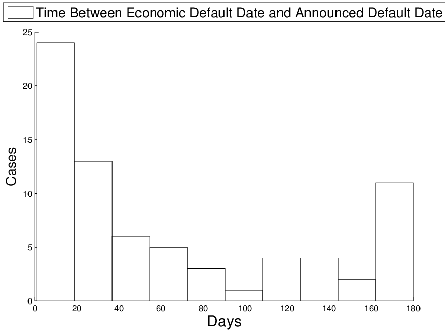
Guo, Jarrow, and Lin’s statistical analysis shows that the time span between the economic and recorded default dates has a significant impact on recovery rate estimates and is key to obtaining unbiased estimates for defaultable bond prices. To illustrate this difference, consider Figure 1. This figure contains a histogram of the time span between the economic and recorded default dates. Of the 96 debt issues studied, 73 trigger economic default strictly before the recorded default date. This difference is significant. Of these 73 issues, 13 have the economic default date at least 180 days before the recorded default date. Capponi (2009) confirms, by a subsequent and different statistical test using credit default swaps (CDS) and equity prices, the market’s pre-knowledge of the onset of default.

Refer to caption — Figure 1: Time between the economic and recorded default dates.

To facilitate future estimation of default times and recovery rates, the purpose of this paper is to develop a theoretical model for a firm’s default process that embeds a distinction between an economic and a recorded default time. To our knowledge, ours is the first paper to provide such a model.

The existing literature on modeling credit risk is extensive, see Jarrow (2010) for a recent review. There are two types of credit risk models: structural and reduced-form. These are related via the information sets available to the management and the market. Reduced form models can be obtained from structural models, by conditioning on the smaller information sets available to the market. In this sense, structural models are the more general approach, from which the reduced form models can be generated. Because we are interested in constructing a new model that includes a distinction between the economic and recorded default dates, we adopt the structural modeling approach. Extensions of our model considering reduced information sets is left for subsequent research.

The initial class of structural models (see, for example, Merton (1974), Black and Cox (1976), Longstaff and Schwartz (1976)) had default occurring when the firm’s asset value hits an exogenously given default barrier. Leland (1994) and Leland and Toft (1996), among others, extended this class of structural models by endogenizing the default barrier. In this extension, the default barrier was selected to maximize the firm’s equity value. For analytical reasons, this extended class of models assumes that the firm’s debt is perpetual and that both the changes in the magnitude and repayment of the firm’s debt is continuous. An implication of this structure is that the firm’s default time can occur at any instant continuously in time.

In contrast, and more consistent with market practice with respect to the repayment of a firm’s debt (both principal and interest), we assume that the firm only makes required debt payments on a set of predetermined discrete times. This simple modification enables us to introduce a distinction between the firm’s economic and recorded default times. In this regard, the recorded default time $\tau_{r}$ is defined to be the first such discrete time that a required debt payment is missed. In contrast, the economic default time $\tau_{e}$ is defined to be the last time prior to $\tau_{r}$ that the firm is able to make such a required debt payment. Since the firm’s management is aware of the fact that this is the last such debt repayment, the economic default time represents the “true” time of default.

Herein, we study the probability distributions of the economic and recorded default times, $\tau_{e}$ and $\tau_{r}$ , respectively. The main analytic difficulty is that $\tau_{e}$ is not a first passage time, but a last passage time given the distribution of $\tau_{r}$ . The key and simple idea underlying our solution is to decompose $\tau_{e}$ into $\tau_{r}-\tau_{e}$ and $\tau_{r}$ . Our primary analytical tool is the fluctuation theory of random walks. The analysis also uses the extensive literature on Lévy processes (see Bertoin (1996) and the references therein), in particular on the links between the law of overshoot for the first passage time and the renewal measures of a Lévy process by Doney and Kyprianou (2006). By studying the distribution of $\tau_{r}-\tau_{e}$ , the time difference between recorded and economic default times, we show that it is a mixture of the arcsine law. This result is (surprisingly) consistent with the empirical observation by Guo, Jarrow, and Lin (2008) (Figure 1).

In addition, we show that the classical structural model can be obtained as a limiting case of our model as the time between the debt repayment dates goes to zero. Our approach illustrates how to use the tail index and correlation structure of the firm’s return to estimate the value process’s parameters (either Brownian motion based or more general Lévy models).

An outline of this paper is as follows. Section 2 presents the model. Section 3 characterizes the distributions for the economic and recorded default times, section 4 relates our model to the classical structural model, and section 5 concludes.

2 The Model

We start with a filtered probability space $(\Omega,\mathcal{F},\mathcal{F}_{t},P)$ that satisfies the usual conditions. Traded are a firm’s asset value process $S_{t}$ and a money market account. Without loss of generality, we assume that the spot rate of interest is zero, so that the money market account has a constant value across time (unity).

2.1 The Firm Value Process

Given a filtered probability space $(\Omega,\mathcal{F},\mathcal{F}_{t},P)$ that satisfies the usual conditions, the value of the firm $S=(S_{t})_{t\geq 0}$ follows a geometric Lévy process together with its natural filtration $({\mathcal{F}}_{t})_{t\geq 0}$ . Specifically, $S_{t}$ is an exponential of a $(b,\sigma,\nu)$ Lévy process, i.e.

S_{t}=S_{0}\exp(X_{t}),

(1)

where

E[e^{i\theta X_{t}}]=e^{t\psi(\theta)},

(2)

with

\psi(\theta)=ib\theta-\frac{\sigma^{2}}{2}\theta^{2}+\int_{(-\infty,\infty)}(e^{i\theta x}-1-i\theta x1_{|x|\leq 1})\nu(dx)+\int_{(-\infty,\infty)}(e^{i\theta x}-1)1_{|x|\leq 1})\nu(dx),

and the jump measure $\nu$ satisfying

\int_{(-\infty,\infty)}(1\wedge x^{2})\nu(dx)<\infty.

Note that $(S_{t},t\geq 0)$ is a martingale if the following condition is satisfied:

b+\dfrac{\sigma^{2}}{2}+\int_{\mathbb{R}}(e^{z}-1-z1_{z\leq 1})\nu(dz)=0.

Consistent with $P$ being an equivalent martingale measure, we assume that this condition is satisfied. This martingale measure need not be unique, so the market need not be complete.

2.2 The Debt Structure

Before introducing the definition of default times, we first need to characterize the firm’s debt structure. We assume that the firm needs to make debt repayments at a predetermined (deterministic) set of discrete times, denoted $N_{1},N_{2},\ldots,N_{n}$ .

For simplicity, let $N_{k}=kN$ for a fixed $N>0$ , which is the time between two consecutive debt repayments (for instance, quarterly). At time $N_{k}$ , the amount of debt in the firm is $D_{k}$ . For simplicity, we assume that $D_{k}=D$ is constant over time.

Consistent with a structural model, the recorded default time $\tau_{r}$ is the first time the firm is unable to make a debt repayment, i.e.

\tau_{r}=\inf\{N_{k},S_{N_{k}}\leq D\}.

(3)

As long as the firm’s asset value exceeds the barrier, it can liquidate assets as necessary to make the debt repayment. Below the barrier, however, it does not have sufficient resources to fulfill its debt obligation.

We define the economic default time to be the last time, before the onset of recorded default, when the firm is able to make a debt repayment, i.e.,

\tau_{e}=\sup_{\tau_{r}\geq t\geq\tau_{r}-N}\{t,S_{t}\geq D\}.

(4)

Since the firm’s management is aware of the fact that this is the last such debt repayment time, the economic default time represents the firm’s “true” default time. In contrast, the recorded default time only corresponds to when this event becomes ”official” and is recorded in both the legal system and the default databases.

The main difference between our model and the classical structural models comes from the discrete debt repayment times. For the existing models, recorded default can happen at any time. In our model, recorded default can only happen at one of the discrete times $N_{k}$ . This discreteness enables us to distinguish between the economic and recorded default times as discussed above.

Remark 2.1.

In Guo, Jarrow, and Lin (2008), the economic default is defined using the entire trajectory of a firm’s bond price until a recorded default occurs in the database. Once recorded default has occurred, one goes backward in time until the discounted price of the bond is the same as the price of an otherwise equivalent defaulted bond. In this paper we provide an economic model for the recorded default time and we define the economic default time using the path of the firm’s value process. Our definition of economic default is consistent with that contained in Guo, Jarrow, and Lin (2008).

3 Computing $\tau_{r}$ and $\tau_{e}$

This section computes the distributions for the recorded default time $\tau_{r}$ , the economic default time $\tau_{e}$ , and relates them to the Arcsine Law. First, note that $\tau_{e}$ is not a stopping time, but rather a last passage time conditioned on the knowledge of $\tau_{r}$ . Direct computation of $\tau_{e}$ seems complicated. To facilitate the computation, we compute $\tau_{e}$ in two steps. First, we we consider $\tau_{r}-\tau_{e}$ . Second, we compute $\tau_{r}$ , which is the first passage time of a random walk. The distribution of $\tau_{e}$ follows naturally from these two steps.

3.1 The Arcsine Law and $\tau_{r}-\tau_{e}$

In this section, we show that the distribution of $\tau_{r}-\tau_{e}$ is a mixture of Arcsine laws.

To start, let us fix some notation. First, we define $(u_{n}(x),n\geq 0)$ to be a sequence of recorded default probabilities. That is, for all $n\geq 0$ ,

u_{n}(x)=\mathbb{P}[\tau_{r}=nN|S_{0}=x]=\mathbb{P}_{x}[\tau_{r}=nN],

(5)

where $\mathbb{P}_{x}$ is the probability measure of the process $(S_{t},t\geq 0)$ conditioned on $S_{0}=x$ .

Note that

\mathbb{P}_{x}[\tau_{r}<\infty]=\sum_{n=1}^{\infty}u_{n}(x)

and for any $0\leq p<k\leq K$ ,

\mathbb{P}_{x}[pN\leq\tau_{r}\leq kN]=\sum_{n=p}^{k}u_{n}(x).

Next, define for $n\geq 0$ the time between real default and economic default conditioned on defaulting at time $nN$ ,

\phi_{n}(x,s)=\mathbb{P}_{x}[\tau_{r}-\tau_{e}\in ds|\tau_{r}=nN].

(6)

In particular, for $x\geq D$ , the probability that default occurs at $t=N$ is

\phi(x,s)=\mathbb{P}_{x}[\tau_{r}-\tau_{e}\in ds|\tau_{r}=N].

(7)

Then by conditioning we have the following relations

\mathbb{P}_{x}[\tau_{r}-\tau_{e}\in ds]=\sum_{n=1}^{\infty}u_{n}(x)\phi_{n}(x,s)ds.

(8)

\mathbb{P}_{x}[\tau_{r}-\tau_{e}\in ds|\tau_{r}<\infty]=\dfrac{\sum_{n=1}^{\infty}u_{n}(x)\phi_{n}(x,s)ds}{\sum_{n=1}^{\infty}u_{n}(x)}.

(9)

Moreover, with the Markov property at time $(n-1)N$ , we see that

\mathbb{P}_{x}[\tau_{r}-\tau_{e}\in ds|\tau_{r}=nN]=\int_{D}^{\infty}\mathbb{P}_{u}[\tau_{r}-\tau_{e}\in ds|\tau_{r}=N]\mathbb{P}_{x}[S_{(n-1)N}\in du|\tau_{r}=nN].

(10)

This suggests that the distribution of $\tau_{e}-\tau_{r}$ is a mixture of the distribution $\phi$ . That is,

Proposition 3.1.

Given a geometric Lévy process $(S_{t},t\geq 0)$ as in expression (1), the distribution of the time between economic and recorded default is given by

\mathbb{P}_{x}[\tau_{e}-\tau_{r}\in ds]=\int_{D}^{\infty}\sum_{n=1}^{\infty}\phi(u,s)u_{n}(x)\mathbb{P}_{x}[S_{(n-1)N}\in du|\tau_{r}=nN].

(11)

Note that the above proposition in fact holds for any time homogeneous stochastic processes with the strong Markov property.

When $(S_{t},t\geq 0)$ is a geometric spectrally positive Levy process, that is, $S_{t}=exp(X_{t})$ with $X=(X_{t})_{t\geq 0}$ a spectrally positive Lévy process, the distribution of $\phi$ can be more explicitly computed. Recall here that a spectrally positive Lévy process $X$ can be represented as:

X_{t}=bt+\sigma W_{t}+J_{t}^{+},

where $W_{t}$ is a standard Brownian motion and $J^{+}=\{J_{t}^{+}\}$ is a non-Gaussian Lévy process with positive jumps.

Proposition 3.2.

Assume that $S=(S_{t},t\geq 0)$ is a geometric spectrally positive Lévy process. Let $S^{\prime}=(S^{\prime}_{t},t\geq 0)$ be an independent copy of $S$ with $S^{\prime}(0)=0$ , then

\phi(x,s)=\mathbb{P}_{x}[\tau_{r}-\tau_{e}\in ds|\tau_{r}=N]=\mathbb{P}[\mathcal{A}_{H_{D}}1_{H_{D}\leq N}\in ds].

(12)

Here

H_{D}=\inf\{t;S_{t}\leq D\}\ \ and\ \ \mathcal{A}_{u}=\inf\{t\leq N-u,\ S^{{}^{\prime}}_{t}\leq 0|S^{{}^{\prime}}_{N-u}\leq 0\}.

(13)

Proof: First, we see that

\phi(x,s)=\mathbb{P}_{x}[\tau_{r}-\tau_{e}\in ds|\tau_{r}=N]=\mathbb{P}_{x}[\tau_{r}-\tau_{e}\in ds|S_{N}\leq D],

because $N$ is the first repayment date.

Therefore conditioned on the first hitting time of $H_{D}$ , we get,

\mathbb{P}_{x}[\tau_{r}-\tau_{e}\in ds|S_{N}\leq D]=\int_{0}^{N}\mathbb{P}_{x}[\tau_{r}-\tau_{e}\in ds|H_{D}\in du;S_{N}\leq D]\mathbb{P}_{x}[H_{D}\in du]

Now, by the strong Markov property at the stopping time $H_{D}$ and $X$ being spectrally positive,

\mathbb{P}_{x}[\tau_{r}-\tau_{e}\in ds|H_{D}\in du;S_{N}\leq D]=\mathbb{P}_{(u,D)}[\tau_{r}-\tau_{e}\in ds|S_{N}\leq D],

where $\mathbb{P}_{(u,D)}$ is the distribution of $S$ starting from $D$ at time $t=u$ . This completes the proof.

Remark 3.3.

Let $S=(S_{t},t\geq 0)$ be a geometric Brownian motion, i.e. $S_{t}=\exp(\mu W_{t}-\mu^{2}t/2)$ under the risk neutral measure for some constant $\mu>0$ with $\{W_{t}\}_{t\geq 0}$ a standard Brownian motion. Then, according to Bentata and Yor (2008) or Madan, Roynette, and Yor (2008),

\mathbb{P}_{(u,D)}[\tau_{e}-\tau_{r}\in ds\ |\tau_{r}=N]=\dfrac{ds}{\pi\sqrt{s(N-u-s)}}\phi(\mu/2\sqrt{N-u-s}).

(14)

with $\phi(\mu)=\int_{0}^{\infty}dte^{-t}\cosh(\mu\sqrt{2t})$ .

3.2 The distribution of $\tau_{r}$

This section focuses on $(\tau_{r},S_{\tau_{r}})$ , the joint distribution of the recorded default time and the value of the firm’s assets. Recall that $(S_{t},t\geq 0)$ is the exponential of a Lévy process. Therefore

(Y_{n})_{n\geq 1}=(\log{S_{nN}}-\log{S_{(n-1)N}})_{n\geq 1}

(15)

is a sequence of i.i.d. random variables with a common distribution $F=^{d}\log(S_{N})$ .

For example, when $\log S_{t}$ is a standard Brownian motion with volatility $\sigma$ , $F=N(0,\sigma N)$ . If $S_{t}$ is the exponential of an $\alpha$ - stable process, then $F$ is an $\alpha$ - stable law.

We now review some relevant notation and a useful lemma for a random walk from fluctuation theory.

For a given random walk $(\log S_{nN},n\geq 0)$ , one considers $T_{n}^{+}$ the $n$ -th time where the random walk $\log S_{nN}$ hits its maximum, and $H_{n}^{+}=\log S_{T_{n}^{+}N}$ , the value of the random walk at that time. Consequently, one defines the increasing ladder time $T^{+}_{n}$ and ladder height process $H^{+}$ as $T^{+}=(T_{n}^{+},n\geq 0)$ and $H^{+}=(H_{n}^{+},n\geq 0)$ where

H_{n}^{+}=\log S_{T_{n}^{+}N},\ T_{n}^{+}=\min\{r>T_{n-1}^{+}:\log S_{rN}>H_{n}^{+}\}

(16)

with $T_{0}^{+}=0.$ Similarly one can define the descending ladder time $T^{-}=(T_{n}^{-},n\geq 1)$ and ladder height process $H^{-}=(H_{n}^{-},n\geq 1)$ as the sequence of consecutive times when the random walk hits its minimum and the values at these minimum.

To study the distribution of the first hitting time of a random walk, it is convenient to consider the Green function of the ladder process of the random walk:

U^{+}(dx,i)=\sum_{n=0}^{\infty}P_{r}(H_{i}^{+}\in dx,\ T_{i}^{+}=n),

(17)

and

U^{-}(dx,i)=\sum_{n=0}^{\infty}P_{r}(H_{i}^{-}\in dx,\ T_{i}^{-}=n).

(18)

The following lemma concerning the first hitting time of a random walk uses the Green function of a ladder process:

Lemma 3.4.

Let $x\geq 0$ and for all $n\geq 0$ , $Z_{n}=\max\{0,\log S_{0},...,\log S_{nN}\}$ , $\bar{\theta}_{n}=\max_{k\leq n}\{\log S_{kN}=Z_{n}\}$ and $\sigma_{x}=\min_{n\geq 1}\{\log S_{nN}>x\}$ , then for all $u>0$ , $y\in[0,x]$ , $v\geq y$ , $i,j\in N$ ,

	$\displaystyle P_{r}(\sigma_{x}-1-\overline{{\theta}_{\sigma_{x-1}}}=i,\bar{\theta}_{\sigma_{x-1}}=j,$		$\displaystyle\log S_{\sigma_{x}N}-x\in du,x-\log S_{(\sigma_{x}-1)N}\in dv,x-Z_{\sigma_{x}-1}\in dy)$
	$\displaystyle=U^{+}(x-dy,j)$		$\displaystyle U^{-}(dv-y,i)F(du+v).$

Immediately, we have

Theorem 3.5.

For any $y>0,k\geq 1$ ,

P_{x}[\tau_{r}=kN,\log S_{\tau_{r}}\in dy]=\sum_{i=0}^{k-1}\int_{\log(D)}^{\log(x)}U^{-}(\log(x/D)-dz,i)\int_{z}^{\infty}U^{+}(du-z,k-i)F(\log(D)-dy-u).

(19)

From a computational perspective, the Green functions can be derived by inverting appropriate Laplace transforms. The following Friedst formula (see [32] for more details) provides an analytical relation between the Green functions of the ladder processes and the distribution of the increments of the random walk.

Theorem 3.6.

(Friedst) For all $(r,t)\in\mathbb{R}^{2},$

1-\mathbb{E}[r^{T_{1}^{+}}e^{itH_{1}^{+}}]=\exp(-\sum_{n=1}^{\infty}\dfrac{r^{n}}{n}\mathbb{E}[e^{it\log(S_{Nn})}:S_{nN}>1]),

(20)

Finally, combining the previous two results, we get the distribution for $\tau_{e}$ .

Corollary 3.7.

$\displaystyle P_{r}(\tau_{e}\in du)$		$\displaystyle=\sum_{k=1}^{\infty}P_{r}[\tau_{e}\in du\|\tau_{r}=kN]P_{r}[\tau_{r}=kN]$
	$\displaystyle=$	$\displaystyle\sum_{k=1}^{\infty}P[\tau_{r}-\tau_{e}\in d(kN-u)\|\tau_{r}=kN]P_{r}[\tau_{r}=kN]$
	$\displaystyle=$	$\displaystyle\sum_{k=1}^{\infty}P[\tau_{r}-\tau_{e}\in d(kN-u)\|\tau_{r}=kN]\int_{0}^{\infty}P[\tau_{r}=kN,S_{\tau_{r}}\in dy]$

where $P[\tau_{r}=kN,S_{\tau_{r}}\in dy]$ follows from Theorem 3.5, and $P[\tau_{r}-\tau_{e}\in ds|\tau_{r}=kN]$ is given by Equation (10) and Proposition 3.2.

3.3 Example

To illustrate the above results, we provide two examples.

Example 3.8.

In this example, we assume that firm’s value $S$ is a geometric Brownian motion with $\sigma=0.25,\mu=0.04$ . We normalize the initial value of the firm to be unity ( $S_{0}=1$ ). The leverage ratio (debt to firm value) is $0.8$ , and the time between debt repayments is $N=15$ days with $D=0.4$ .

Example 3.9.

In this example, we again assume that the dynamic of the firm’s value is a geometric Brownian motion with $\sigma=0.25,\mu=0.04$ . The leverage ratio is 0.8 and $N=3$ months with $D=0.1.$

4 Relation with the Classical Structural Models

In the classical structural models, the recorded default time is modeled as the first hitting time of a diffusion process (with possible jumps) to a default barrier in continuous time. In this section, we show that when appropriately re-scaling the time step, our discrete model and the recorded default time asymptotically approaches the classical definition of the recorded default when the time step goes to zero. A useful corollary of our approach is that one can use the tail index and correlation structure of $Y_{i}$ to estimate the parameters of the firm value process (either Brownian motion based or more general Lévy models).

To start, consider a firm which reveals information only at the discrete times $Nk$ for $k\geq 0$ . The information is the current asset value $S_{Nk}$ . Define for all $k\geq 1$ , $\log(\dfrac{S_{Nk}}{S_{N(k-1)}})=Y_{k}$ , “the firm’s return”, with the sequence $(Y_{k},k\geq 1)$ being stationary. The debt is refinanced and rolls over at these times $Nk$ and without loss of generality $r=0$ .

Next, define $P_{x}^{N}(T_{1},T_{2})$ to be the probability that recorded default will occur between $T_{1}$ and $T_{2}$ for any given $T_{2}>T_{1}>0$ , i.e.,

P_{x}^{N}(T_{1},T_{2})=\mathbb{P}_{x}[T_{1}<\tau_{r}\leq T_{2}].

(21)

Now consider the following re-scaling:

•

re-scaling $N$ by a factor of $n$ with $N\mapsto N/n$ , and
•

re-scaling the firm’s return by a factor $\zeta_{n}$ (to be determined) with $Y_{k}\mapsto\dfrac{Y_{k}}{\zeta_{n}}$ ,

so that for all $n\geq 1$ ,

S_{t}^{n}=S_{0}^{n}\exp(\sum_{k=1}^{[nt/N]}\dfrac{Y_{k}}{\zeta_{n}}).

(22)

Under the risk neutral measure, $S^{n}$ becomes

S_{t}^{n}=S_{0}^{n}\exp(\sum_{k=1}^{[nt/N]}\dfrac{Y_{k}}{\zeta_{n}}-\phi_{n}(t)),

(23)

where for all $n\geq 1$ ,

\phi_{n}(t)=\log(\ \mathbb{E}[\exp(\ \sum_{k=1}^{[nt/N]}\dfrac{Y_{k}}{\zeta_{n}})]).

(24)

A simple application of the invariance principle will show that this rescaling function $(\zeta_{n},n\geq 1)$ is a function of the tail exponent of the return sequence $(Y_{k},k\geq 1)$ .

Proposition 4.1.

If the sequence $(Y_{n},n\geq 1)$ is a sequence of weakly dependent (such as uniformly) stationary random variables with

\mathbb{E}[Y_{1}^{2}]+2\sum_{k=2}^{\infty}Cov(Y_{1},Y_{i})=\sigma^{2}<\infty,

(25)

then $\zeta_{n}=\sqrt{n}$ and

(S^{n}_{t},t\geq 0)\Rightarrow\exp(\dfrac{\sigma}{\sqrt{N}}B_{t}-t\dfrac{\sigma^{2}}{2N}),

(26)

where the convergence is in distribution on the Skorokhod space $\mathcal{D}$ . Moreover for all $T_{1}<T_{2}$ ,

P_{x}^{N/n}(T_{1},T_{2})\rightarrow_{n\to\infty}\int_{T_{1}}^{T_{2}}p(x,s,\dfrac{\sigma}{\sqrt{N}})ds,

(27)

for all $0\leq s\leq\infty$ , with $p(x,s,\dfrac{\sigma}{\sqrt{N}})$ the first hitting time probability density function of $\exp(\dfrac{\sigma}{\sqrt{N}}B_{t}-t\dfrac{\sigma^{2}}{2N})$ starting from x hitting the level $D$ .

Proof. First, let $\mathbb{E}[Y_{i}]=\mu$ , one has from theorem 4.4.1 from [44]

(\dfrac{Y_{1}+...+Y_{[nt]}-[nt]\mu}{\sqrt{n}},t\geq 0)\Rightarrow(\sigma B_{t},t\geq 0)\ \ \mbox{on}\ (\mathcal{D},J_{1}).

(28)

Therefore, by continuity of the exponential function on the Skorokhod space, one has

(\exp(\sum_{i=0}^{[nt/N]}\dfrac{Y_{i}}{\sqrt{n}}-t\phi_{n}),t\geq 0)\Rightarrow\exp(\dfrac{\sigma}{\sqrt{N}}B_{t}-t\dfrac{\sigma^{2}}{2N})\ \ \mbox{on}\ (\mathcal{D},J_{1}).

(29)

Moreover, since the first hitting time is a continuous function on the Skorokhod space,

P_{x}^{N/n}(T_{1},T_{2})\rightarrow_{n\to\infty}\int_{T_{1}}^{T_{2}}p(x,s,\dfrac{\sigma}{\sqrt{N}})ds,

(30)

where for all $0\leq s\leq\infty$ , $p(x,s,\dfrac{\sigma}{\sqrt{N}})$ is given by

p(x,s,\dfrac{\sigma}{\sqrt{N}})=\dfrac{\log(D/x)}{\sqrt{2\pi N}s^{3/2}\sigma}\exp(-\dfrac{(\dfrac{\log(D/x)}{\sqrt{N}\sigma}+\dfrac{\sigma s}{2\sqrt{N}})^{2}}{2s})

(31)

Remark 4.2.

When $N$ goes to zero, where the dynamics of the firm value follows a geometric Brownian motion, it is clear $\tau_{r}-\tau_{e}=0$ almost surely.

When the sequence $(Y_{i},i\geq 1)$ does not have a moment of order two, we see that

Proposition 4.3.

Y_{1}+...+Y_{n}=^{d}n^{1/\alpha}Y_{1},

(32)

for $\alpha\in(0,2)$ then $\zeta_{n}=n^{1/\alpha}$ and

S^{n}\Rightarrow\exp(S^{\alpha}_{t}-tC_{\alpha})\ \ \mbox{on}\ (\mathcal{D},J_{1}),

(33)

where $C_{\alpha}$ is a constant depending on the characteristics of the stable process $S^{\alpha}$ , with $\tau_{r}=\tau_{e}=\inf\{t,S_{t}\leq D\}$ . ²² 2 This is known as $\alpha$ -stable distribution, which is generally represented as a four-parameter family: the index, the scale, the skewness and the shift parameter. For more details, see for instance [41] and [44]).

Remark 4.4.

The previous proposition links the volatility coefficient of the firm value process $\sigma_{f}$ as a function of the variance of its return $Y_{i}$ and $N$ so that

\sigma_{f}^{2}=\dfrac{\mathbb{E}[Y_{1}^{2}]+2\sum_{k=2}^{\infty}Cov(Y_{1},Y_{k})}{N}.

(34)

Thus, one can use the tail index of $Y_{1}$ and the correlation structure of the sequence $(Y_{i},i\geq 1)$ to estimate the parameters of the firm’s value process.

5 Conclusion

This paper develops a structural credit risk model to characterize the difference between the economic and recorded default times for a firm. Recorded default occurs when default is recorded in the legal system. The economic default time is when the market first prices the firm’s debt as if it has defaulted. It has been empirically documented that these two times are distinct (see Guo, Jarrow, and Lin (2008)). In our model, this distinction is obtained by assuming that debt repayments occur on a set of discrete dates, and not continuously as in the classical structural models. We show that the probability distribution for the time span between economic and recorded defaults follows a mixture of Arcsine Law, which is consistent with the results contained in Guo, Jarrow, and Lin. In addition, we show that the classical structural model can be obtained as a limiting case of our model as the time between the debt repayment dates goes to zero. We also illustrate how to estimate the parameters of the firm value process using the time series of the firm’s return. Our model is a first step in characterizing the difference between the economic and recorded default times. Our simple model can be generalized in numerous ways, and we hope to pursue these extensions in subsequent research.

References

[1] Ammann, M. (2001) Credit Risk Valuation. Springer.
[2] Artzner, P. and Delbaen, F. (1995) Default risk insurance and incomplete market. Mathematical Finance, 5, 187–195.
[3] Bélanger, A., Shreve, S., and Wong, D. (2004) A general framework for pricing credit risk. Mathematical Finance, 14(3), 317–350.
[4] Bentata, A. and Yor, M. (2008) From Black-Scholes and Dupire formulae to last passage times of local martingales. Working paper.
[5] Bertoin, J. (1995) Sample path behaviour in connection with generalized arcsine laws. Probability Theory and Related Fields. 103(3), 317–327.
[6] Bertoin, J. (1996) Lévy Processes. Cambridge Univ. Press.
[7] Bharath, S. and Shumway, T. (2008) Forecasting default with the Merton distance to default model. Review of Financial Studies, 21 (3), 1339 - 1369.
[8] Bielecki, T. and Rutkowski, R. (2002) Credit Risk: Modeling, Valuation, and Hedging. Springer.
[9] Black, F. and Cox, J. (1976) Valuing corporate securities: some effects of bond indenture provisions, Journal of Finance, 31, 351 - 367.
[10] Campbell, J., Hilscher, J. , and J. Szilagyi. (2006) In search of distress risk. Journal of Finance, 63 (6), 2899 - 2939.
[11] Capponi, A. (2009) Does equity market reveal information before any other market: a comparison between news revelation of CDS and equity market. Private communication, Goldman Sachs, London.
[12] Capponi, A. and Cvitanić, J. (2009) Credit risk modeling with misreporting and incomplete information. International Journal of Theoretical and Applied Finance, 12, 81-112.
[13] Çetin, U., Jarrow, R., Protter, P., and Yildirim, Y. (2004) Modeling credit risk with partial information. Annals of Applied Probability, 14, 1167–1178.
[14] Chava, S. and Jarrow, R (2004) Bankruptcy prediction with industry effects. Review of Finance, 8 (4), 537-569.
[15] Chava, S., Stefanescu, C., and Turnbull, S. (2006) Modeling expected loss. Working paper, Bauer College of Business.
[16] Collin-Dufresne, P., Goldstein, R., and Helwege, J. (2004) Is credit event risk priced? Modeling contagion via the updating of beliefs. Working paper, Carnegie Mellon University.
[17] Doney, R. A. and Kyprianou, A. E. (2006) Overshoots and undershoots of Lévy processes. Annals of Applied Probability, 16(1):91–106.
[18] Duffie, D. and Lando, D. (2001) Term structures of credit spreads with incomplete accounting information. Econometrica, 69(3):633–664.
[19] Duffie, D. and Singleton, K. (1999) Modeling term structure of defaultable bonds. Review of Financial Studies, 12, 687–720.
[20] Duffie, D. and Singleton, K. (2003) Credit Risk. Princeton University Press.
[21] Elliott, R. J., Jeanblanc, M., and Yor, M. (2000) On models of default risk. Mathematical Finance, 10(2):179–195.
[22] Giesecke, K. (2006) Default and information. Journal of Economic Dynamics and Control, 30(11), 2281-2303.
[23] Guo, X., and Jarrow, R., and Lin, H. Z. (2008) Distressed debt prices and recovery rate estimation. Review of Derivatives Research, 11(3):171–204.
[24] Ikeda, N. and Watanabe, S. (1989) Stochastic Differential Equations and Diffusion Processes, North-Holland, Second Edition,
[25] Jarrow, R. (2010) Credit risk models. Annual Review of Financial Economics, 1, 37 - 68.
[26] Jarrow, R. and Protter, P. (2004) Structural versus reduced-form models: a new information based perspective, Journal of Investment Management, 2(2), 34–43.
[27] Jarrow, R. and Turnbull, S. (1992) Credit risk: drawing the analogy. Risk Magazine, 5(9).
[28] Jarrow, R. and Turnbull, S. (1995) Pricing options of financial securities subject to default risk. Journal of Finance, 50:53–86.
[29] Karatzas, I. and Shreve, S. (1997) Stochastic Calculus and Brownian Motion. Springer.
[30] Kallenberg O. (2001) Foundations of Modern Probability. Springer.
[31] Klüppelberg, C., Kyprianou, A. E., and Maller, R. A. (2004) Ruin probabilities and overshoots for general Lévy processes. Annals of Applied Probability, 14:1766–1801.
[32] Kyprianou, A. E. (2006), Introductory Lectures on Fluctuations of Lévy Processes with Applications. Springer.
[33] Lando, D. (1998) Cox processes and credit-risky securities. Review of Derivatives Research, 2, 99–120.
[34] Lando, D. (2004) Credit Risk Modeling: Theory and Applications. Princeton University Press.
[35] Leland, H. (1994) Corporate debt value, bond covenants, and optimal capital structure. Journal of finance, 49(4):1213–1252.
[36] Leland, H. and Toft, K. B. (1996) Optimal capital structure, endogenous bankruptcy. and the term structure of credit spreads. Journal of Finance, 51(3):987–1019.
[37] Longstaff, F. and Schwartz, E. (1995) A Simple approach to valuing risky fixed and floating rate debt, Journal of Finance, 50 (3), 789 - 819.
[38] Madan, D., Roynette, B., and Yor, M. (2008) From Black–Scholes formula, to local times and last passage times for certain submartingales. Working paper.
[39] Mansuy, R. and Yor, M. (2006) Random Times and Enlargements of Filtrations in a Brownian Setting. Lecture Notes in Mathematics, No. 1873, Springer.
[40] Merton, R. C. (1974) On the pricing of corporate debt: the risk structure of interest rates, Journal of Finance, 29, 449 - 470.
[41] Samorodnitsky, G. and Taqqu, M. S. (1994) Stable Non-Gussian Random Processes. Chapman-Hall.
[42] Schönbucher, P. J. (2003) Credit Derivatives Pricing Models. Wiley.
[43] Spitzer, F. (1975) Principles of Random Walk. Springer-Verlag.
[44] Whitt, W. (2002) Stochastic Process Limits. Springer-Verlag.