The coupling of topology and inflation in noncommutative cosmology
Abstract.
We show that, in a model of modified gravity based on the spectral action functional, there is a nontrivial coupling between cosmic topology and inflation, in the sense that the shape of the possible slow-roll inflation potentials obtained in the model from the nonperturbative form of the spectral action are sensitive not only to the geometry (flat or positively curved) of the universe, but also to the different possible non-simply connected topologies. We show this by explicitly computing the nonperturbative spectral action for some candidate flat cosmic topologies given by Bieberbach manifolds and showing that the resulting inflation potential differs from that of the flat torus by a multiplicative factor, similarly to what happens in the case of the spectral action of the spherical forms in relation to the case of the -sphere. We then show that, while the slow-roll parameters differ between the spherical and flat manifolds but do not distinguish different topologies within each class, the power spectra detect the different scalings of the slow-roll potential and therefore distinguish between the various topologies, both in the spherical and in the flat case.
1. Introduction
Noncommutative cosmology is a new and rapidly developing area of research, which aims at building cosmological models based on a “modified gravity” action functional which arises naturally in the context of noncommutative geometry, the spectral action functional of [4]. As we discuss more in detail in §2 below, this functional recovers the usual Einstein–Hilbert action, with additional terms, such as a conformal gravity, Weyl curvature term. It also has the advantage of allowing for interesting couplings of gravity to matter, when extended from manifolds to “almost commutative geometries” as in [7] and later models [6], [3]. Thus, this approach makes it possible to recover from the same spectral action functional, in addition to the gravitational terms, the full Lagrangian of various particle physics models, ranging from the Minimal Standard Model of [7], to the extension with right handed neutrinos and Majorana mass terms of [6], and to supersymmetric QCD as in [3]. The study of cosmological models derived from the spectral action gave rise to early universe models as in [15] and [11], which present various possible inflation scenarios, as well as effects on primordial black holes evaporation and gravitational wave propagation. Effects on gravitational waves, as well as inflation scenarios coming from the spectral action functional, were also recently studied in [17], [18], [19].
Our previous work [16] showed that, when one considers the nonperturbative form of the spectral action, as in [5], one obtains a slow-roll potential for inflation. We compared some of the more likely candidates for cosmic topologies (the quaternionic and dodecahedral cosmology, and the flat tori) and we showed that, in the spherical cases (quaternionic and dodecahedral), the nonperturbative spectral action is just a multiple of the spectral action of the sphere , and consequently the inflation potential only differs from the one of the sphere case by a constant scaling factor, which cancels out in the computation of the slow-roll parameters, which are therefore the same as in the case of a simply connected topology and do not distinguish the different cosmic topologies with the same spherical geometry.
This result for spherical space forms was further confirmed and extended in [25], where the nonperturbative spectral action is computed explicitly for all the spherical space forms and it is shown to be always a multiple of the spectral action of , with a proportionality factor that depends explicitly on the 3-manifold. Thus, different candidate cosmic topologies with the same positively curved geometry yield the same values of the slow-roll parameters and of the power-law indices and tensor-to-scalar ratio, which are computed from these parameters.
In [16], however, we showed that the inflation potential obtained from the nonperturbative spectral action is different in the case of the flat tori, and not just by a scalar dilation factor. Thus, we know already that the possible inflation scenarios in noncommutative cosmology depend on the underlying geometry (flat or positively curved) of the universe, and the slow–roll parameters are different for these two classes.
The slow-roll parameters alone only distinguish, in our model, between the flat and spherical geometries but not between different topologies within each class. However, in the present paper we show that, when one looks at the amplitudes for the power spectra for density perturbations and gravitational waves (scalar and tensor perturbations), these detect the different scaling factors in the slow-roll potentials we obtain for the different spherical and flat topologies, hence we obtain genuinely different inflation scenarios for different cosmic topologies.
We achieve this result by relying on the computations of the nonperturbative spectral action, which in the spherical cases are obtained in [16] and [25], and by deriving in this paper the analogous explicit computation of the nonperturbative spectral action for the flat Bieberbach manifolds. A similar computation of the spectral action for Bieberbach manifolds was simultaneously independently obtained by Piotr Olczykowski and Andrzej Sitarz in [20].
Thus, the main conclusion of this paper is that a modified gravity model based on the spectral action functional predicts a coupling between cosmic topology and inflation potential, with different scalings in the power spectra that distinguish between different topologies, and slow-roll parameters that distinguish between the spherical and flat cases.
The paper is organized as follows. We first describe in §1.1 the broader context in which the problem we consider here falls, namely the cosmological results relating inflation, the geometry of the universe, and the background radiation, and the problem of cosmic topology. We then review briefly in §2 the use of the spectral action as a modified gravity functional and the important distinction between its asymptotic expansion at large energies and the nonperturbative form given in terms of Dirac spectra. In §4 we present the main mathematical result of this paper, which gives an explicit calculation of the nonperturbative spectral action for certain Bieberbach manifolds, using the Dirac spectra of [21] and a Poisson summation technique similar to that introduced in [5], and used in [16] and [25].
Finally, in §6 we compare the resulting slow-roll inflation potentials, power spectra for density perturbations and slow-roll parameters, for all the different possible cosmic topologies.
1.1. Inflation, geometry, and topology
It is well known that the mechanism of cosmic inflation, first proposed by Alan Guth and Andrei Linde, naturally leads to a flat or almost flat geometry of the universe (see for instance §1.7 of [14]). It was then shown in [10] that the geometry of the universe can be read in the cosmic microwave background radiation (CMB), by showing that the anisotropies of the CMB depend primarily upon the geometry of the universe (flat, positively or negatively curved) and that this information can be detected through the fact that the location of the first Doppler peak changes for different values of the curvature and is largely unaffected by other parameters. This theoretical result made it possible to devise an observational test that could confirm the inflationary theory and its prediction for a flat or nearly flat geometry. The experimental confirmation of the nearly flat geometry of the universe came in [2] through the Boomerang experiment. Thus, the geometry of the universe leaves a measurable trace in the CMB, and measurements confirmed the flat geometry predicted by inflationary models.
The cosmic topology problem instead concentrates not on the question about the curvature and the geometry of the universe, but on the possible existence, for a given geometry, of a non-simply connected topology, that is, of whether the spatial sections of spacetime can be compact 3-manifolds which are either quotients of the 3-sphere (spherical space forms) in the positively curved case, quotients of 3-dimensional Euclidean space (flat tori or Bieberbach manifolds) in the flat case, or quotients of the 3-dimensional hyperbolic space (hyperbolic 3-manifolds) in the negatively curved space. A general introduction to the problem of cosmic topology is given in [12].
Since the cosmological observations prefer a flat or nearly flat positively curved geometry to a nearly flat negatively curved geometry (see [2], [27]), most of the work in trying to identify the most likely candidates for a non-trivial cosmic topology concentrate on the flat spaces and the spherical space forms. Various methods have been devised to try to detect signatures of cosmic topology in the CMB, in particular through a detailed analysis of simulated CMB skies for various candidate cosmic topologies (see [22] for the flat cases). It is believed that perhaps some puzzling features of the CMB such as the very low quadrupole, the very planar octupole, and the quadrupole–octupole alignment may find an explanation in the possible presence of a non-simply connected topology, but no conclusive results to that effect have yet been obtained.
The recent results of [16] show that a modified gravity model based on the spectral action functional imposes constraints on the form of the possible inflation slow-roll potentials, which depend on the geometry and topology of the universe, as shown in [16]. While the resulting slow-roll parameters and spectral index and tensor-to-scalar ratio distinguish the even very slightly positively curved case from the flat case, these parameters alone do not distinguish between the different spherical topologies, as shown in [25]. As we show in this paper, the situation is similar for the flat manifolds: these same parameters alone do not distinguish between the various Bieberbach manifolds (quotients of the flat torus), but they do distinguish these from the spherical quotients. However, if one considers, in addition to the slow-roll parameters, also the power spectra for the density fluctuations, one can see that, in our model based on the spectral action as a modified gravity functional, the resulting slow-roll potentials give different power spectra that distinguish between all the different topologies.
1.2. Slow-roll potential and power spectra of fluctuations
We first need to recall here some well known facts about slow-roll inflation potentials, slow-roll parameters, and the power spectra for density perturbations and gravitational waves. We refer the reader to [23] and to [13], [24], as well as to the survey of inflationary cosmology [1].
Consider an expanding universe, which is topologically a cylinder , for a -manifold , with a Lorentzian metric of the usual Friedmann form
| (1.1) |
where is the Riemannian metric on the -manifold .
In models of inflation based on a single scalar field slow-roll potential , the dynamics of the scale factor in the Friedmann metric (1.1) is related to the scalar field dynamics through the acceleration equation
| (1.2) |
where is the Hubble parameter, which is related to the scalar field and the inflation potential by
| (1.3) |
and is the slow-roll parameter, which depends on the potential as described in (1.11) below, see [1] for more details.
It is customary to decompose perturbations of the metric of (1.1) into scalar and tensor perturbations, which correspond, respectively, to density fluctuations and gravitational waves. One typically neglects the remaining vector components of the perturbation, assuming that these are not generated by inflation and decay with the expansion of the universe, see §9.2 of [1]. Thus, one writes scalar and tensor perturbations in the form
| (1.4) |
with and , and where the give the tensor part of the perturbation, satisfying and . The tensor perturbations have two polarization modes, which correspond to the two polarizations of the gravitational waves.
One considers then the intrinsic curvature perturbation
| (1.5) |
which measures the spatial curvature of a comoving hypersurface, that is, a hypersurface with constant . After expanding in Fourier modes in the form
| (1.6) |
one obtains the power spectrum for the density fluctuations (scalar perturbations of the metric) from the two-point correlation function,
| (1.7) |
In the case of a Gaussian distribution, the power spectrum describes the complete statistical information on the perturbations, while the higher order correlations functions contain the information on the possible presence of non-Gaussianity phenomena. The power spectrum for the tensor perturbations is similarly obtained by expanding the tensor fluctiations in Fourier modes and computing the two-point correlation function
| (1.8) |
In slow-roll inflation models, the power spectra and are related to the slow-roll potential through the leading order expression (see [23])
| (1.9) |
up to a constant proportionality factor, and with the Planck mass. Here the potential and its derivative are to be evaluated at where the corresponding scale leaves the horizon during inflation. These can be expressed a power law as ([23])
| (1.10) |
where the spectral parameters , , , and depend on the slow–roll potential in the following way. In the slow-roll approximation, the slow-roll parameters are given by the expressions
| (1.11) |
Notice that we follow here a different convention with respect to the one we used in [16] on the form of the slow-roll parameters. The spectral parameters are then obtained from these as
| (1.12) |
while the tensor-to-scalar ratio is given by
| (1.13) |
From the point of view of our model, the following observation will be useful when we compare the slow-roll potentials that we obtain for different cosmic topologies and how they affect the power spectra.
Lemma 1.1.
Proof.
This is an immediate consequence of (1.9), (1.11), (1.12), and (1.10). In fact, from (1.9), we see that maps , and also , since it transforms . On the other hand, the expressions and and in the slow-roll parameters (1.11) are left unchanged by , so that the slow-roll parameters and all the resulting spectral parameters of (1.12) are unchanged. Thus, the power law (1.10) only changes by a multiplicative factor and , with unchanged exponents. ∎
2. Noncommutative cosmology
2.1. The spectral action as a modified gravity model
In its nonperturbative form, the spectral action is defined in terms of the spectrum of the Dirac operator, on a spin manifold or more generally on a noncommutative space (a spectral triple), as the functional , where is a smooth test function and is an energy scale that makes dimensionless.
The reason why this can be regarded as an action functional for gravity (or gravity coupled to matter in the noncommutative case) lies in the fact that, for large energies it has an asymptotic expansion (see [4]) of the form
| (2.1) |
with and with the integrations
given by residues of zeta function at the positive points of the dimension spectrum of the spectral triple, that is, the set of poles of the zeta functions. In the case of a 4-dimensional spin manifold, these, in turn, are expressed in terms of integrals of curvature terms. These include the usual Einstein–Hilbert action
and a cosmological term
but it also contains some additional terms, like a non-dynamical topological term
where denotes the form that represents the Pontrjagin class and integrates to a multiple of the Euler characteristic of the manifold, as well as a conformal gravity term
which is given in terms of the Weyl curvature tensor. We do not give any more details here and we refer the reader to Chapter 1 of [CoMa] for a more complete treatment.
The presence of conformal gravity terms along with the Einstein–Hilbert and cosmological terms give then a modified gravity action functional. When one considers the nonperturbative form of the spectral action, rather than its asymptotic expansion at large energies, one can find additional nonperturbative correction terms. One of these was identified in [5], in the case of the 3-sphere, as a potential for a scalar field, which was interpreted in [16] as a potential for a cosmological slow-roll inflation scenario, and computed for other, non-simply connected cosmic topologies.
3. Geometry, topology and inflation: spherical forms
The nonperturbative spectral action for the spherical space forms was computed recently by one of the authors [25]. It turns out that, although the Dirac spectra can be significantly different for different spin structures, the spectral action itself is independent of the choice of the spin structure, and it is always equal to a constant multiple of the spectral action for the 3-sphere , where the multiple is just dividing by the order of the group . This is exactly what one expects by looking at the asymptotic expansion of the spectral action for large energies , and the only significant nonperturbative effect arises in the form of a slow-roll potential, as in [5], [16].
Theorem 3.1.
(Teh, [25]) For all the spherical space forms with the round metric induced from , and for all choices of spin structure, the nonperturbative spectral action on is equal to
| (3.1) |
up to order .
Correspondingly, as explained in §5 of [16], one obtains a slow-roll potential by considering the variation of the spectral action as in [5]. More precisely, one considers a Euclidean compactification of the 4-dimensional spacetime to a compact Riemannian manifold with the compactification of size . One then computes the spectral action on this compactification and its variation
| (3.2) |
up to terms of order , where the potential is given by the following.
Proposition 3.2.
Let be a spherical space form with the induced round metric. Let be the radius of the sphere and the size of the circle in the Euclidean compactification . Then the slow-roll potential in (3.2) is of the form
| (3.3) |
where
| (3.4) |
with
| (3.5) |
and with
| (3.6) |
In particular, for the different spherical forms, the potential has the same form as that of the 3-sphere case, but it is scaled by the factor ,
| (3.7) |
Notice, moreover, that in the potential one has an overall factor of that multiplies the term and a factor of that multiplies the term. As we observed already in [16], when one Wick rotates back to the Minkowskian model with the Friedmann metric, both the scale factor and the energy scale evolve with the expansion of the universe, but in such a way that so that the product . In [16] we did not need to analyze the behavior of the factor, since we only looked at the slow-roll parameters (1.11) where that factor cancels out. In the spectral action model of cosmology, the choice of the scale of the Euclidean compactification is an artifact of the model, which allows one to compute the spectral action in terms of the spectrum of the Dirac operator on the compact Riemannian 4-manifold . Eventually, the physically significant quantities derived from the spectral action functional are Wick rotated back to the Minkowskian signature case. Since in its nonperturbative form the spectral action functional is supposed to give a modified gravity action functional that works at all scales, not just in the asymptotic expansion for large , it seems therefore natural to set the choice of the length in the model so that the product remains constant.
Another reason for making the assumption that is the interpretation given in [5] of the parameter in the Euclidean compactification as an inverse temperature. Then, up to a universal constant, that behaves like the inverse of an energy scale and, when rotating back to the Minkowskian signature, one knows that, in the expansion of the universe the scale factor is inversely proportional to the temperature, so that the assumption is justified.
With this setting, the slow-roll potential one obtains in the case of the 3-sphere is of the form
| (3.8) |
Then one has the following result for the power spectra for the various cosmic topology candidates given by spherical space forms.
Proposition 3.3.
Let and denote the power spectra for the density fluctuations and the gravitational waves, computed as in (1.9), for the slow-roll potential . Then they satisfy the power law
| (3.9) |
where for and the spectral parameters , , , are computed as in (1.12) from the slow-roll parameters (1.11), which satisfy , , .
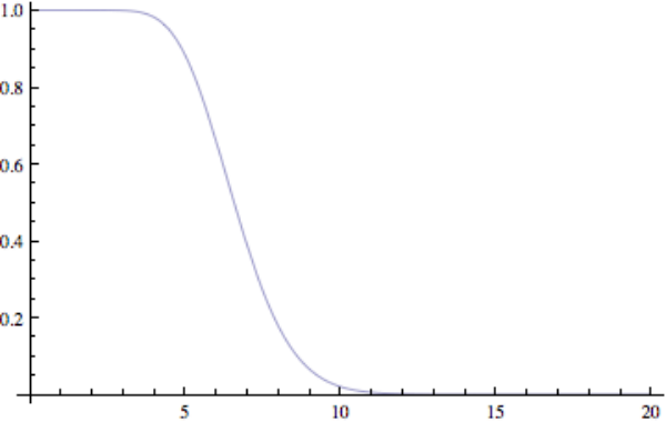
To see explicitly the effect on the slow-roll potential of the scaling by , we consider the same test functions used in [5] to approximate smoothly a cutoff function. These are given by
Figure 1 shows the graph of when . We use this test function to compute the slow-roll potential using the function , after setting the factors and , and up to an overall multiplicative factor of . We then see in Figure 2 the different curves of the slow-roll potential for the three cases where with the binary tetrahedral, binary octahedral, or binary icosahedral group, respectively given by the top, middle, and bottom curve.

4. The spectral action for Bieberbach manifolds
We now consider the case of candidate cosmic topologies that are flat 3-manifolds. The simplest case is the flat torus , which we have already discussed in [16]. There are then the Bieberbach manifolds, which are obtained as quotients of the torus by a finite group action. In this section we give an explicit computation of the nonperturbative spectral action for the Bieberbach manifolds (with the exception of which requires a different technique and will be analyzed elsewhere), and in the next section we then derive the analog of Proposition 3.3 for the case of these flat geometries.
Calculations of the spectral action for Bieberbach manifolds were simultaneously independently obtained in [20].
The Dirac spectrum of Bieberbach manifolds is computed in [21] for each of the six affine equivalence classes of three-dimensional orientable Bieberbach manifolds, and for each possible choice of spin structure and choice of flat metric. These classes are labeled through , with simply being the flat 3-torus.
In general, the Dirac spectrum for each space depends on the choice of spin structure. However, as in the case of the spherical manifolds, we show here that the nonperturbative spectral action is independent of the spin structure.
We follow the notation of [21], according to which the different possibilities for the Dirac spectra are indicated by a letter (e.g. ). Note that it is possible for several spin structures to yield the same Dirac spectrum.
The nonperturbative spectral action for was computed in [16]. We recall here the result for that case and then we restrict our discussion to the spaces through .
4.1. The structure of Dirac spectra of Bieberbach manifold
The spectrum of the Bieberbach manifolds generally consists of a symmetric component and an asymmetric component as computed in [21]. The symmetric components are parametrized by subsets , such that the eigenvalues are given by some formula , , and the multiplicity of each eigenvalue, , is some constant times the number of such that . In the case of , , , the constant is , while in the case the constant is .
The approach we use here to compute the spectral action nonperturbatively consists of using the symmetries of as a function of to almost cover all of the points in and then apply the Poisson summation formula as used in [5]. By “almost cover”, it is meant that it is perfectly acceptable if two-, one-, or zero-dimensional lattices through the origin are covered multiple times, or not at all.
The asymmetric component of the spectrum appears only some of the time. The appearance of the asymmetric component depends on the choice of spin structure. For those cases where it appears, the eigenvalues in the asymmetric component consist of the set
where is a constant depending on the spin structure, and is given in the following table:
| Bieberbach manifold | |
For no choice of spin structure does have an asymmetric component to its spectrum. Each of the eigenvalues in has multiplicity . Using the Poisson summation formula as in [5], we see that the asymmetric component of the spectrum contributes to the spectral action
| (4.1) |
The approach described here is effective for computing the nonperturbative spectral action for the manifolds labeled in [21] as , but not for . Therefore, we do not consider the case in this paper: it will be discussed elsewhere.
4.2. Recalling the torus case
We gave in Theorem 8.1 of [16] the explicit computation of the non-perturbative spectral action for the torus. We recall here the statement for later use.
Theorem 4.1.
Let be the flat torus with an arbitrary choice of spin structure. The nonperturbative spectral action is of the form
| (4.2) |
up to terms of order .
4.3. The spectral action for
The Bieberbach manifold is the one that is described as “half-turn space” in the cosmic topology setting in [22], because the identifications of the faces of the fundamental domain is achieved by introducing a -rotation about the -axis. It is obtained by considering a lattice with basis , , and , with and , and then taking the quotient of by the group generated by the commuting translations along these basis vectors and an additional generator with relations
| (4.3) |
Like the torus , the Bieberbach manifold has eight different spin structures, parameterized by three signs , see Theorem 3.3 of [21]. Correspondingly, as shown in Theorem 5.7 of [21], there are four different Dirac spectra, denoted , , , and , respectively associated to the the spin structures
We give the computation of the nonperturbative spectral action separately for each different spectrum and we will see that the result is independent of the spin structure and always a multiple of the spectral action of the torus.
4.3.1. The case of
In this first case, we go through the computation in full detail. The symmetric component of the spectrum is given by the data ([21])
We make the assumption that . Set . Then we have equivalently:
Theorem 4.2.
Let be the Bieberbach manifold , with and with a spin structure with . The nonperturbative spectral action of the manifold is of the form
| (4.4) |
up to terms of order .
Proof.
We compute the contribution to the spectral action due to . Since is invariant under the transformation and , we see that
The decomposition of used to compute this contribution to the spectral action is displayed in figure 4. Applying the Poisson summation formula we get a contribution to the spectral action of
plus possible terms of order .
As for we again use the fact that the spectrum is invariant under the transformation , to see that
The decomposition for this contribution to the spectral action is displayed in figure 3. We get a contribution to the spectral action of
plus possible terms of order .
When we include the contribution (4.1) due to the asymmetric component we see that the spectral action of the space G2-(a) is equal to
again up to possible terms of order . ∎


4.3.2. The case of and
The spectra of and have no asymmetric component. The symmetric component is given by
Let us once again assume that .
Theorem 4.3.
Let and be the Bieberbach manifolds , with and with a spin structure with and , respectively. The nonperturbative spectral action of the manifolds and is again of the form
| (4.5) |
up to terms of order .
Proof.
With the assumption that and letting , we can describe the spectrum equivalently by
Using the symmetry
we cover exactly, (see figure 5) and we obtain the spectral action
∎

4.3.3. The case of
In this case, the symmetric component of the spectrum is given by
Again, we assume .
Theorem 4.4.
Let be the Bieberbach manifolds , with and with a spin structure with . The nonperturbative spectral action of the manifold is again of the form
| (4.6) |
up to terms of order .
Proof.
If we substitute , we see that we may equivalently express the symmetric component with
Using the symmetry
we cover exactly (see figure 6), and so the spectral action is again given by
∎

4.4. The spectral action for
The Bieberbach manifold is the one that, in the cosmic topology setting of [22] is described as the “third-turn space”. One considers the hexagonal lattice generated by vectors , and , for and in , and one then takes the quotient of by the group generated by commuting translations along the vectors and an additional generator with relations
| (4.7) |
This has the effect of producing an identification of the faces of the fundamental domain with a turn by an angle of about the -axis, hence the “third-turn space” terminology.
As shown in Theorem 3.3 of [21], the Bieberbach manifold has two different spin structures, parameterized by one sign . It is then shown in Theorem 5.7 of [21] that these two spin structures have different Dirac spectra, which are denoted as and . We compute below the nonperturbative spectral action in both cases and we show that, despite the spectra being different, they give the same result for the nonperturbative spectral action, which is again a multiple of the action for the torus.
4.4.1. The case of and
The symmetric component of the spectrum is given by
| (4.8) |
| (4.9) |
with for the spin structure and for the spin structure .
The manifold is unusual in that the multiplicity of is equal to twice the number of elements in which map to it.
Theorem 4.5.
On the manifold with an arbitrary choice of spin structure, the non-perturbative spectral action is given by
| (4.10) |
plus possible terms of order .
Proof.
Notice that is invariant under the linear transformations , given by
Let .
Therefore the symmetric component of the spectrum contributes to the spectral action
Combining this with the asymmetric contribution (4.1), we see that the spectral action of spaces and is equal to
Now, if one makes the change of variables , where
then the spectral action becomes
∎
Notice that, a priori, one might have expected a possibly different result in this case, because the Bieberbach manifold is obtained starting from a hexagonal lattice rather than the square lattice, but up to a simple change of variables in the integral, this gives again the same result, up to a multiplicative constant, as in the case of the standard flat torus.

4.5. The spectral action for
The Bieberbach manifold is referred to in [22] as the “quarter-turn space”. It is obtained by considering a lattice generated by the vectors , , and , with , and taking the quotient of by the group generated by the commuting translations along the vectors and an additional generator with the relations
| (4.12) |
This produces an identification of the sides of a fundamental domain with a rotation by an angle of about the -axis. Theorem 3.3 of [21] shows that the manifold has four different spin structures parameterized by two signs . There are correspondingly two different forms of the Dirac spectrum, as shown in Theorem 5.7 of [21], one for , the other for , denoted by and .
Again the nonperturbative spectral action is independent of the spin structure and equal in both cases to the same multiple of the spectral action for the torus.
4.5.1. The case of
Theorem 4.6.
On the manifold with a spin structure with , the non-perturbative spectral action is given by
| (4.13) |
plus possible terms of order .
Proof.
The symmetric component of the spectrum is given by
First, we make the change of variables . Then we use the symmetries
to cover all of except for the one-dimensional lattice . This decomposition is depicted in figure 8. In the figure one sees that the points such that are covered twice, and the points such that are not covered at all, but via the transformation , this is the same as covering each of the points , once. Observations like this will be suppressed in the sequel. Then we see that the contribution from the symmetric component of the spectrum to the spectral action is
| (4.14) |
up to terms of order . Combining this with the asymmetric component, we find that the spectral action is given by (4.13). ∎

4.5.2. The case of
In this case there is no asymmetric component in the spectrum. The symmetric component is given by the data
We again obtain the same expression as in the case for the spectral action.
Theorem 4.7.
On the manifold with a spin structure with , the non-perturbative spectral action is also given by
| (4.15) |
up to possible terms of order .
Proof.

Remark 4.8.
The technique we use here to sum over the spectrum to compute the non-perturbative spectral action does not appear to work in the case of the Bieberbach manifold , which is the “sixth-turn space” described from the cosmic topology point of view in [22], namely the quotient of by the group generated by commuting translations along the vectors , and , , and an additional generator with , and , which produces an identification of the faces of the fundamental domain with a -turn about the -axis. This case will therefore be analyzed elsewhere, but it is reasonable to expect that it will also give a multiple of the spectral action of the torus, with a proportionality factor of .
4.6. The spectral action for
We analyze here the last remaining case of compact orientable Bieberbach manifold , the Hantzsche–Wendt space, according to the terminology followed in [22]. This is the quotient of by the group obtained as follows. One considers the lattice generated by vectors , , and , with , and the group generated by commuting translations along these vectors, together with additional generators , , and with the relations
| (4.16) |
This gives an identification of the faces of the fundamental domain with a twist by an angle of along each of the three coordinate axes.
According to Theorems 3.3 and 5.7 of [21], the manifold has four different spin structures parameterized by three signs subject to the constraint , but all of them yield the same Dirac spectrum, which has the following form.
The manifold also has no asymmetric component to its spectrum, while the symmetric component is given by
We then obtain the following result.
Theorem 4.9.
The Bieberbach manifold with an arbitrary choice of spin structure has nonperturbative spectral action of the form
| (4.17) |
up to terms of order .
Proof.

5. Geometry, topology and inflation: flat manifolds
As shown in Theorem 8.3 of [16], on a flat torus of sides the slow roll potential is of the form
with given by
| (5.1) |
as in (3.6).
Proposition 5.1.
Proof.
We the obtain the following analog of Proposition 3.3 in the flat case.
Proposition 5.2.
Let and denote the power spectra for the density fluctuations and the gravitational waves, computed as in (1.9), for the slow-roll potential . Then they satisfy the power law
| (5.5) |
where is as in (5.4), for a Bieberbach manifold and the spectral parameters , , , are computed as in (1.12) from the slow-roll parameters (1.11), which satisfy , , .
If one assumes that each of the characteristic sizes involved, , , would be comparable to , after Wick rotating from Euclidean to Lorentzian signature, as in the expansion scale , one would then obtain proportionality factors that are simply of the form
| (5.6) |
Assuming then that , and using the same test function with as in Figure 1 we then obtain different curves as in Figure 11 for the case (top curve), case (middle curve), and for the and cases (bottom curve).

6. Conclusions: Inflation potential, power spectra, and cosmic topologies
We have seen in this paper that, in a modified gravity model based on the non-perturbative spectral action functional, different cosmic topologies, either given by spherical space forms or by flat Bieberbach manifolds, leave a signature that can distinguish between the different topologies in the form of the slow roll inflation potential that is obtained from the variation of the spectral action functional. The amplitude of the potential, and therefore the amplitude of the corresponding power spectra for density perturbations and gravitational waves (scalar and tensor perturbations), differs by a factor that depends on the topology, while the slow-roll parameters only detect a difference between the spherical and flat cases. As one knows from [13], [23], [24], both the slow-roll parameters and the amplitude of the power spectra are constrained by cosmological information, so in this kind of modified gravity model, one in principle obtains a way to constrain the topology of the universe based on the slow-roll inflation potential, on the slow-roll parameters and on the power spectra for density perturbations and gravitational waves. The factors that correct the amplitudes depending on the topology are given by the following table.
| spherical | flat | ||
|---|---|---|---|
| sphere | flat torus | ||
| lens | |||
| binary dihedral | |||
| binary tetrahedral | |||
| binary octahedral | ? | ||
| binary icosahedral |
Notice that some ambiguities remain: the form of the potential and the value of the scale factor alone do not distinguish, for instance, between a lens space with , a binary dihedral quotient with and the binary tetrahedral quotient, or between the Poincaré dodecahedral space (the binary icosahedral quotient), a lens space of order and a binary dihedral quotient with . At this point we do not know whether more refined information can be extracted from the spectral action that can further distinguish between these cases, but we expect that, when taking into account a more sophisticated version of the spectral action model, where gravity is coupled to matter by the presence of additional (non-commutative) small extra-dimensions (as in [6], [7]), one may be able to distinguish further. In fact, instead of a trivial product , one can include the non-commutative space using a topologically non-trivial fibration over the 4-dimensional spacetime and this allows for a more refines range of proportionality factors . We will discuss this in another paper.
References
- [1] D. Baumann, TASI Lectures on inflation, Lectures from the 2009 Theoretical Advanced Study Institute at Univ. of Colorado, Boulder, arXiv:0907.5424 [160 pages].
- [2] P. de Bernardis, P.A.R. Ade, J.J. Bock, J.R. Bond, J. Borrill, A. Boscaleri, K. Coble, B.P. Crill, G.De Gasperis, P.C. Farese, P.G. Ferreira, K. Ganga, M. Giacometti, E. Hivon, V.V. Hristov, A. Iacoangeli, A.H. Jaffe, A.E. Lange, L. Martinis, S. Masi, P.V. Mason, P.D. Mauskopf, A. Melchiorri, L. Miglio, T. Montroy, C.B. Netterfield, E. Pascale, F. Piacentini, D. Pogosyan, S. Prunet, S. Rao, G. Romeo, J.E. Ruhl, F. Scaramuzzi, D. Sforna, N. Vittorio, A flat Universe from high-resolution maps of the cosmic microwave background radiation, Nature 404 (2000), 955–959.
- [3] T. van den Broek, W.D. van Suijlekom, Supersymmetric QCD and noncommutative geometry, arXiv:1003.3788.
- [4] A. Chamseddine, A. Connes, The spectral action principle. Comm. Math. Phys. 186 (1997), no. 3, 731–750.
- [5] A. Chamseddine, A. Connes, The uncanny precision of the spectral action, Commun. Math. Phys. 293 (2010) 867–897.
- [6] A. Chamseddine, A. Connes, M. Marcolli, Gravity and the standard model with neutrino mixing, Adv. Theor. Math. Phys. 11 (2007), no. 6, 991–1089.
- [7] A. Connes, Gravity coupled with matter and foundation of noncommutative geometry. Commun. Math. Phys., 182 (1996) 155–176.
- [8] G.I. Gomero, M.J. Reboucas, R. Tavakol, Detectability of cosmic topology in almost flat universes, Class. Quant. Grav. 18 (2001) 4461–4476.
- [9] G.I. Gomero, M.J. Reboucas, A.F.F. Teixeira, Spikes in cosmic crystallography II: topological signature of compact flat universes, Phys. Lett. A 275 (2000) 355–367.
- [10] M. Kamionkowski, D.N. Spergel, N. Sugiyama, Small-scale cosmic microwave background anisotropies as a probe of the geometry of the universe, Astrophysical J. 426 (1994) L 57–60.
- [11] D. Kolodrubetz, M. Marcolli, Boundary conditions of the RGE flow in the noncommutative geometry approach to particle physics and cosmology, Phys. Lett. B693 (2010) 166–174.
- [12] M. Lachièze-Rey, J.P. Luminet, Cosmic topology. Physics Reports, 254 (1995) 135–214.
- [13] J.E. Lidsey, A.R. Liddle, E.W. Kolb, E.J. Copeland, T. Barreiro, M. Abney, Reconstructing the Inflaton Potential – an Overview, Rev. Mod. Phys (1997) Vol.69, 373–410.
- [14] A. Linde, Particle physics and inflationary cosmology, CRC Press, 1990.
- [15] M. Marcolli, E. Pierpaoli, Early universe models from noncommutative geometry, arXiv:0908.3683.
- [16] M. Marcolli, E. Pierpaoli, K. Teh, The spectral action and cosmic topology, arXiv:1005.2256, to appear in Communications in Mathematical Physics.
- [17] W. Nelson, J. Ochoa, M. Sakellariadou, Gravitational Waves in the Spectral Action of Noncommutative Geometry, arXiv:1005.4276
- [18] W. Nelson, J. Ochoa, M. Sakellariadou, Constraining the Noncommutative Spectral Action via Astrophysical Observations, Phys. Rev. Lett. Vol. 105 (2010) 101602 [5 pages].
- [19] W. Nelson, M. Sakellariadou, Natural inflation mechanism in asymptotic noncommutative geometry, Phys. Lett. B (2009) Vol.680, 263–266.
- [20] Piotr Olczykowski, Andrzej Sitarz, On spectral action over Bieberbach manifolds, arXiv:1012.0136.
- [21] F. Pfäffle, The Dirac spectrum of Bieberbach manifolds, J. Geom. Phys. 35 (2000) 367–385.
- [22] A. Riazuelo, J. Weeks, J.P. Uzan, R. Lehoucq, J.P. Luminet, Cosmic microwave background anisotropies in multiconnected flat spaces, Phys. Rev. D 69 (2004) 103518 [25 pages].
- [23] T.L. Smith, M. Kamionkowski, A. Cooray, Direct detection of the inflationary gravitational wave background, Phys. Rev. D (2006) Vol.73, N.2, 023504 [14 pages].
- [24] E.D. Stewart, D.H. Lyth, A more accurate analytic calculation of the spectrum of cosmological perturbations produced during inflation, Phys. Lett. B 302 (1993) 171–175.
- [25] K. Teh, Nonperturbative Spectral Action of Round Coset Spaces of , arXiv:1010.1827.
- [26] J.P. Uzan, U. Kirchner, Ulrich, G.F.R. Ellis, WMAP data and the curvature of space, Mon. Not. Roy. Astron. Soc. 344 (2003) L65.
- [27] M. White, D. Scott, E. Pierpaoli, Boomerang Returns Unexpectedly, The Astrophysical Journal, 545 (2000) 1–5.