The Quantum Field as a Quantum Computer

Giacomo Mauro D’Ariano Affiliation: QUIT Group, Dipartimento di Fisica “A. Volta”, via Bassi 6, I-27100 Pavia, Italy Affiliation: Istituto Nazionale di Fisica Teorica e Nucleare, Sezione di Pavia.

Abstract

It is supposed that at very small scales a quantum field is an infinite homogeneous quantum computer. On a quantum computer the information cannot propagate faster than $c=a/\tau$ , $a$ and $\tau$ being the minimum space and time distances between gates, respectively. It is shown that the information flow satisfies a Dirac equation, with speed $v=\zeta c$ and $\zeta=\zeta(m)$ mass-dependent. For $a/\tau=c$ the speed of light $\zeta^{-1}$ is a vacuum refraction index increasing monotonically from $\zeta^{-1}(0)=1$ to $\zeta^{-1}(M)=\infty$ , $M$ being the Planck mass for $2a$ the Planck length.

pacs

11.10.-z,03.70.+k,03.67.Ac,03.67.-a,04.60.Kz

It is interesting to explore the possibility that pure information may underlie all of physics. From what we know, such information should be made of quantum bits (qubits), instead of classical bits. A fundamental problem is then to establish if there is something more than Quantum Theory in a quantum field. Can we say that a quantum field is just a collection of (infinitely many) quantum systems, each at every “space point” (a Planck cell), unitarily interacting with a bunch of other systems? Does the continuum play a fundamental role, or it is only a mathematical idealization? Are space, time, and all physical observables emergent features of a quantum information processing?

Looking at physics as pure information processing means to consider qubits as primitive entities. In simple words: qubits are not supported by “matter”, but matter is made of quantum information patterns. This is the It from bit of Wheeler [1]. At the opposite side of pure speculation, the new information paradigm has an enormous foundational power, reducing the fundamental theoretical framework of physics to quantum theory only, and forcing the definition of each physical quantity to be given in operational terms [2, 3]. This is for example the spirit of the Seth Lloyd’s proposal of basing a theory of quantum gravity on a quantum computation [4]. The quantum computational network is just the causal network from which the geometry of space-time should be derived. The idea of deriving the geometry of space from causal networks is a program initiated by Rafael Sorkin and collaborators more than two decades ago [5]. More recently the Lorentz transformations have been explicitly derived from a causal network with topological homogeneity [6], thus showing how relativity can be regarded as emergent from the quantum computation (a “visual” proof of time-dilation and space-contraction was given in Ref. [7]). The main idea is that causality naturally endows foliations on the causal network [8, 9], and the choice of a foliation on a computational circuit corresponds to synchronize subroutine calls to a global clock in a distributed computation [10].

In this paper I will consider an unbounded quantum circuit that is dynamically homogeneous, and, for simplicity, with the topology of gate connections that can be embedded in two dimensions—the equivalent of 1+1 dimensions. All the results (apart from maybe anticommuting fields) can be generalized to more than one space dimension. The dynamical homogeneity of the quantum circuit represents the equivalent of the physical law, which is supposed to hold everywhere and forever. In such a way the circuit will incarnate a quantum field theory at some very small scale, e.g. the Planck scale [11]. We will see that the information flow along the circuit naturally satisfies a Dirac-like equation. And, as an observable consequence of the unitariety of the evolution, one has a renormalization of the speed of light, resulting in a vacuum refraction index which depends on the mass of the field, and which effective stops the flow of information at the Planck mass.

In the (one-dimensional) quantum computer information can flow only in two directions—right and left—at the speed $a/\tau$ of one-gate-per-step. Mathematically we describe the information flows in the two directions by the two field operators $\phi^{+}$ and $\phi^{-}$ , for the right and the left propagation, respectively. In equations one has

\widehat{\partial}_{t}\begin{bmatrix}\phi^{+}\\ \phi^{-}\end{bmatrix}=\begin{bmatrix}c\widehat{\partial}_{x}&0\\ 0&-c\widehat{\partial}_{x}\end{bmatrix}\begin{bmatrix}\phi^{+}\\ \phi^{-}\end{bmatrix},

(1)

where $c=a/\tau$ is the speed of the flow over the network, and the hat on the partial derivative will remind us that they are indeed finite-difference, generally extended to more than one gate (see the following). If we take the maximal information speed $a/\tau=c$ as a universal constant, then $c$ must be equal to the speed of light. Now, the only way of slowing-down the information flow is to have it changing direction repeatedly. A constant average speed corresponds to a simply periodic change of direction, which is described mathematically by a coupling between $\phi^{+}$ and $\phi^{-}$ with an imaginary constant. Upon denoting by $\omega$ the angular frequency of such periodic change of direction, we have

\widehat{\partial}_{t}\begin{bmatrix}\phi^{+}\\ \phi^{-}\end{bmatrix}=\begin{bmatrix}c\widehat{\partial}_{x}&-i\omega\\ -i\omega&-c\widehat{\partial}_{x}\end{bmatrix}\begin{bmatrix}\phi^{+}\\ \phi^{-}\end{bmatrix}.

(2)

The slowing down of information propagation can be considered as the informational meaning of inertial mass, and $\omega$ represents its value. Notice that Eq. (2) is nothing but the Dirac equation (without spin), which means that the quantum-information processing corresponding to pure information transfer simulates a Dirac field—the periodic change of direction being the Zitterbewegung [12]. It is worth emphasizing that Eq. (2) has been derived only as a general description of a uniform information transfer, without requiring Lorentz covariance.

The analogy with the Dirac equation leads us to write the coupling constant in terms of the Compton wavelength $\lambda=c\omega^{-1}=\hbar/(mc)$ . This allows us to establish the following relation between $m$ and $\omega$

m=\frac{\tau^{2}}{a^{2}}\hbar\omega=\frac{1}{c^{2}}\hbar\omega.

(3)

Eq. (3) provides an informational meaning to the Planck constant $\hbar$ as the conversion factor between the informational notion of inertial mass in sec^-1 and its customary notion in Kg. Also note that equivalence between the two notions of mass in Eq. (3) corresponds to the Planck quantum expressed as rest energy.

I will now show that the unitariety of the information flows produces a renormalization of $c$ when introducing the coupling $\omega$ , namely the Dirac equation (3) becomes

i\widehat{\partial}_{t}\phi=(ic\zeta\sigma_{3}\widehat{\partial}_{x}+\omega\sigma_{1})\phi,\quad\phi=\begin{bmatrix}\phi^{+}\\ \phi^{-}\end{bmatrix}

(4)

where $0<\zeta=\zeta(\omega)\leq 1$ and $\zeta=1$ only for $\omega=0$ .

Different from a quantum field, in a quantum computation there is no Hamiltonian, since, in order to have finite average information speed with $\tau$ non infinitesimal, all the gates must produce a transformation far from the identity. We can define a local Hamiltonian matrix in terms of the discrete time-derivative of the field as

{\rm H^{(2n)}_{gate}}z:=i\frac{z(n\tau)-z(-n\tau)}{2n\tau}=:i\widehat{\partial}_{t}z.

(5)

We are interested in a field evolution linear in the field, whence we restrict attention to gate unitary operators $U$ that transform the fields linearly as $z_{n}(t=1)=Uz_{n}U^{\dagger}=\sum_{k}U_{nk}z_{k}$ , $\{z_{k}\}$ denoting the field operators involved by the gate. Clearly, the the matrix $\mathbf{U}:=\|U_{ij}\|$ must be itself unitary, and this will also guarantee preservation of (anti)commutation relations for the field. By taking the adjoint we get $z_{i}(t=-1)=\sum_{j}U_{ij}^{\dagger}z_{j}$ . By composing the evolution from many gates we derive the path-sum rules:

Refer to caption — Figure 1: Rule for numbering wires to evaluate the contribution of each gate to the forward evolution of the field operator $y$ (left) and to the backward evolution of $x$ (right).

Path-sum rule for the forward evolution:

1) Number all the input wires at each gate, from the leftmost to the rightmost one, and do the same for the output wires, as in Figs. 1 and 2. 2) We say that a wire $l$ is in the past-cone of the wire $k$ if there is a path from $l$ to $k$ passing through gates.

3) For any output wire $k$ and any input wire $l$ in its causal past cone, consider all paths connecting $k$ with $l$ , and denote them as follows (see Fig. 2)

\mathbf{i}_{kl}=(i_{1}i_{2}\ldots i_{n}i_{n+1})\;\text{with}\;i_{1}=k,\;i_{n+1}=l,

(6)

4) The following linear expansion holds

z_{l}(t)=\sum_{\mathbf{i}_{kl}}U^{(1)}_{i_{1}i_{2}}U^{(2)}_{i_{2}i_{3}}\ldots U^{(n)}_{i_{n}i_{n+1}}z_{k}(0)

(7)

where $U_{i_{m}i_{m+1}}$ is the matrix element of the $m$ -th gate crossed by the path, from the $i_{m}$ -th output wire to the $i_{m+1}$ -th input wire.

Rule for evaluating the backward evolution:

1) For any input wire $l$ and any output wire $k$ in the causal future cone of $l$ , consider all paths passing through gates connecting $k$ with $l$ (see Fig. 2)

\mathbf{i}_{lk}=(i_{n+1}i_{n}\ldots i_{2}i_{1})\;\text{with}\;i_{n+1}=l,\;i_{1}=k.

(8)

2) The following linear expansion holds

z_{l}(-t)=\sum_{\mathbf{i}_{lk}}U^{(n){\dagger}}_{i_{n+1}i_{n}}U^{(n-1){\dagger}}_{i_{n}i_{n-1}}\ldots U^{(1)}_{i_{2}i_{1}}z_{k}(0).

(9)

We now derive the field equation corresponding to a quantum circuit describing the interaction between a left and right-propagating field operators $\phi^{\pm}$ . It is sufficiently general to consider alternate uniform rows of gates, with unitary interactions $\mathbf{A}$ and $\mathbf{B}$ as in Fig. 3. Using the rules for evolution of the field, one has

		$\displaystyle\begin{bmatrix}\phi^{+}\\ \phi^{-}\end{bmatrix}_{t=2}=$	$\displaystyle\begin{bmatrix}A_{21}B_{21}\widehat{\partial}_{-}+A_{22}B_{11}&A_{21}B_{22}\widehat{\partial}_{-}+A_{22}B_{12}\\ A_{11}B_{21}+A_{12}B_{11}\widehat{\partial}_{+}&A_{11}B_{22}+A_{12}B_{12}\widehat{\partial}_{+}\end{bmatrix}$	$\displaystyle\begin{bmatrix}\phi^{+}\\ \phi^{-}\end{bmatrix},$		(10)
		$\displaystyle\begin{bmatrix}\phi^{+}\\ \phi^{-}\end{bmatrix}_{t=-2}=$	$\displaystyle\begin{bmatrix}B^{\dagger}_{12}A^{\dagger}_{12}\widehat{\partial}_{+}+B^{\dagger}_{11}A^{\dagger}_{22}&B^{\dagger}_{11}A^{\dagger}_{21}\widehat{\partial}_{-}+B^{\dagger}_{12}A^{\dagger}_{11}\\ B^{\dagger}_{21}A^{\dagger}_{22}+B^{\dagger}_{22}A^{\dagger}_{12}\widehat{\partial}_{+}&B^{\dagger}_{22}A^{\dagger}_{11}+B^{\dagger}_{21}A^{\dagger}_{21}\delta^{-}\end{bmatrix}$	$\displaystyle\begin{bmatrix}\phi^{+}\\ \phi^{-}\end{bmatrix}$		(11)

where $\partial_{\pm}$ denotes the shift operators $\partial_{\pm}\vec{\phi}_{n}:=\vec{\phi}_{n\pm 1}$ . According to our definition of Hamiltonian in Eq. (5), we have

{\rm H^{(4)}_{gate}}=\tfrac{i}{4\tau}\begin{bmatrix}A_{21}B_{21}\widehat{\partial}_{-}-B^{\dagger}_{12}A^{\dagger}_{12}\widehat{\partial}_{+}+A_{22}B_{11}-B^{\dagger}_{11}A^{\dagger}_{22}&(A_{21}B_{22}-B^{\dagger}_{11}A^{\dagger}_{21})\widehat{\partial}_{-}+A_{22}B_{12}-B^{\dagger}_{12}A^{\dagger}_{11}\\ (A_{12}B_{11}-B^{\dagger}_{22}A^{\dagger}_{12})\widehat{\partial}_{+}+A_{11}B_{21}-B^{\dagger}_{21}A^{\dagger}_{22}&A_{12}B_{12}\widehat{\partial}_{+}-B^{\dagger}_{21}A^{\dagger}_{21}\widehat{\partial}_{-}+A_{11}B_{22}-B^{\dagger}_{22}A^{\dagger}_{11}\end{bmatrix}.

(12)

It is easy to check that the Hamiltonian is Hermitian, e. g. $\langle\phi_{n}^{\pm}|{\rm H^{(4)}_{gate}}|\phi_{n}^{\pm}\rangle=\langle\phi_{n}^{\pm}|{\rm H^{(4)}_{gate}}|\phi_{n}^{\pm}\rangle^{*}$ , $\langle\phi_{n+1}^{\pm}|{\rm H^{(4)}_{gate}}|\phi_{n}^{\pm}\rangle=\langle\phi_{n}^{\pm}|{\rm H^{(4)}_{gate}}|\phi_{n+1}^{\pm}\rangle^{*}$ , etc. In the following we will denote the coarse-grained discrete space-derivative as $\widehat{\partial}_{x}=\frac{1}{4a}(\widehat{\partial}_{+}-\widehat{\partial}_{-})$ ( $a$ distance between centers of n.n. gates: see Fig. 3). The Hamiltonian ${\rm H^{(4)}_{gate}}$ has the Dirac form (4) if

{\rm H^{(4)}_{gate}}=c(\mathbf{H}+i\mathbf{K}\widehat{\partial}_{x}),

(13)

where

\mathbf{H}:=\begin{bmatrix}H_{11}&H_{12}\\ H_{12}^{*}&H_{22}\end{bmatrix},\;\mathbf{K}:=\begin{bmatrix}K_{11}&K_{12}\\ -K_{12}^{*}&K_{22}\end{bmatrix},

(14)

and

\begin{split}H_{11}=&-\tfrac{1}{2a}\Im(A_{21}B_{21}+A_{22}B_{11})=0,\\ H_{12}=&\tfrac{i}{4a}(A_{21}B_{22}-A^{*}_{12}B^{*}_{11}+A_{22}B_{12}-A^{*}_{11}B^{*}_{21})=\lambda^{-1},\\ H_{22}=&-\tfrac{1}{2a}\Im(A_{12}B_{12}+A_{11}B_{22})=0,\\ K_{11}=&-\Re(A_{21}B_{21})=\zeta,\\ K_{22}=&\Re(A_{12}B_{12})=-\zeta,\\ K_{12}=&-\tfrac{1}{2}(A_{21}B_{22}-A^{*}_{12}B^{*}_{11})=0.\end{split}

(15)

namely

\begin{split}&A_{21}B_{22}=A^{*}_{12}B^{*}_{11},\\ &A_{21}B_{21}+A_{22}B_{11},A_{12}B_{12}+A_{11}B_{22}\in\mathbb{R},\\ &\Re(A_{21}B_{21})=\Re(A_{12}B_{12})=-\zeta,\\ &A_{22}B_{12}-A^{*}_{11}B^{*}_{21}=-4ia\lambda^{-1}.\end{split}

(16)

Unitarity of $\mathbf{A}$ and $\mathbf{B}$ means

\begin{split}&|A_{11}|^{2}+|A_{12}|^{2}=|A_{21}|^{2}+|A_{22}|^{2}=1,\\ &A_{11}A^{*}_{21}+A_{12}A^{*}_{22}=A_{21}A^{*}_{11}+A_{22}A^{*}_{12}=0,\end{split}

(17)

and similarly for $\mathbf{B}$ . Without loss of generality, we can take the determinants $|\mathbf{A}|=|\mathbf{B}|=1$ , corresponding to $A_{11}=A_{22}^{*}$ , $A_{12}=-A_{21}^{*}$ , and similarly for $\mathbf{B}$ . The first of identities (16) then gives $B_{11}=B_{22}=0$ , whence

\begin{split}&B_{11}=B_{22}=0,\quad A_{12}B_{12}=A_{21}B_{21}=-\zeta,\\ &A_{22}B_{12}=-A_{11}^{*}B_{21}^{*}=-2ia\lambda^{-1}.\\ \end{split}

(18)

Upon parametrizing $\mathbf{A}$ and $\mathbf{B}$ as follows

\mathbf{A}=\begin{bmatrix}e^{i\phi}\cos\theta&e^{i\psi}\sin\theta\\ -e^{-i\psi}\sin\theta&e^{-i\phi}\cos\theta\end{bmatrix},\;\mathbf{B}=\begin{bmatrix}0&e^{i\xi}\\ -e^{-i\xi}&0\end{bmatrix},

(19)

one obtains

e^{i(\psi+\xi)}=-1,\quad e^{i(\phi-\xi)}=i,

(20)

and

\sin\theta=\zeta=\sqrt{1-\left(\frac{2a}{\lambda}\right)^{2}}.

(21)

Eq. (21) corresponds to a mass-dependent vacuum refraction index $\zeta^{-1}$ which is strictly greater than 1 (apart from the special case of zero mass), and monotonically increasing versus the mass and infinite (i.e. no propagation of information) for $\lambda\to 2a$ . Notice also that for $m=0$ both unitaries become swaps, modulo a phase.

The existence of a vacuum refraction index is a general feature of the discreteness of quantum information processing, and comes from imposing that the maximum information speed $a/\tau$ cannot be greater than the speed of light. The refraction index is simply a consequence of unitarity and linearity in the field operators, independently on the details of the circuit. Indeed, an upper bound for $\zeta$ holding for any circuit can be established as follows. In order to obtain Eq. (4) we need a gate Hamiltonian ${\rm H^{(2n)}_{gate}}=ic\zeta\sigma_{3}\widehat{\partial}_{x}+\omega\sigma_{1}$ . The Hamiltonian is Hermitian, whence $U_{f}=U_{b}$ . Moreover, we must have the same number $n$ of time-steps $\tau$ and of space-steps $a$ , and from the form of the Hamiltonian we get $n=2$ . We thus have

{\rm H^{(4)}_{gate}}=\frac{i}{4\tau}(U_{f}-U_{f}^{\dagger})

(22)

and taking the norm of both sides we obtain

|\!|{\rm H^{(4)}_{gate}}|\!|\leq\frac{1}{2\tau}

(23)

The norm is obtained by Fourier transform at wave-vector $k=\pi/(4a)$ , giving

\frac{\sqrt{\zeta^{2}+4\tau^{2}\omega^{2}}}{2\tau}\leq\frac{1}{2\tau},

(24)

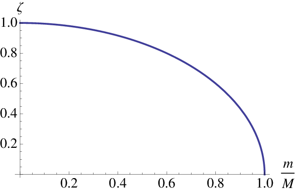
namely for $\omega=c\lambda^{-1}$ one has $\zeta\leq\sqrt{1-\left(\frac{2a}{\lambda}\right)^{2}}$ .

Up to now we have considered only an abstract unitary transformation of the field $\phi=(\phi^{+},\phi^{-})$ . We want now to address the problem of the operator algebras that are actually processed by the gates. Without loss of generality in the following we will fix the phase $\phi=0$ , whence $\xi=\psi=-\pi/2$ . It is easy to show that for field operators $z,z^{\prime}$ either Bose or Fermi the following identity holds

e^{\alpha^{*}z^{\prime{\dagger}}z-\alpha z^{\dagger}z^{\prime}}ze^{\alpha z^{\dagger}z^{\prime}-\alpha^{*}z^{\prime{\dagger}}z}=\cos|\alpha|\,z+\frac{\alpha}{|\alpha|}\sin|\alpha|\,z^{\prime}.

(25)

It follows that the unitary operators corresponding to gates $A$ and $B$ have the operator form

\begin{split}A=&\exp\left\{i\theta\left[\phi_{n}^{+}{}^{\dagger}\phi_{n-1}^{-}+\phi_{n-1}^{-}{}^{\dagger}\phi_{n}^{+}\right]\right\},\\ B=&\exp\left\{i\tfrac{\pi}{2}\left[\phi_{n}^{+}{}^{\dagger}\phi_{n}^{-}+\phi_{n}^{-}{}^{\dagger}\phi_{n}^{+}\right]\right\},\end{split}

(26)

where we omit the index $n$ labeling the unitary. The field operators can be written as local operators in the Bose case, e. g. $\phi_{n}^{+}=a_{2n}$ and $\phi_{n}^{-}=a_{2n+1}$ , with $a_{l}$ harmonic-oscillator operators $[a_{l},a_{k}^{\dagger}]=\delta_{lk}$ . In the Fermi case we can use the Clifford algebraic construction

\phi_{n}^{+}=\sigma_{2n}^{-}\prod_{k=-\infty}^{2n-1}\sigma_{k}^{3},\quad\phi_{n}^{-}=\sigma_{2n+1}^{-}\prod_{k=-\infty}^{2n}\sigma_{k}^{3}.

(27)

and find

\begin{split}A=&\exp\left[-i\theta\left(\sigma_{2n-1}^{-}\sigma_{2n}^{+}+\sigma_{2n-1}^{+}\sigma_{2n}^{-}\right)\right],\\ B=&\exp\left[-i\tfrac{\pi}{2}\left(\sigma_{2n}^{+}\sigma_{2n+1}^{-}+\sigma_{2n}^{-}\sigma_{2n+1}^{+}\right)\right].\\ &\end{split}

(28)

Therefore, upon associating each wire of the circuit to a local algebra of Pauli matrices, the gate unitary operators are functions only of the local algebras of their wires. For the vacuum we can select any state that is left invariant by the quantum computation. In particular, we can choose $|\mathbf{0}\rangle=\prod_{k}|0\rangle_{k}$ which is annihilated by the logarithm of either $A$ and $B$ , and similarly for the Bose field. It is easy to see that $N=\sum_{n}\sigma_{n}^{3}$ ( $N=\sum_{n}a_{n}^{\dagger}a_{n}$ for Bose) is a constant of motion, which can be interpreted as the number of particles. Notice that for a given field theory to be simulable by a homogeneous quantum computer in the discrete approximation $\phi(na)=a^{-\frac{1}{2}}\phi_{n}$ , one needs the field Hamiltonian $H$ (giving $i\partial_{t}\phi=[H,\phi]$ ) that can be written as $H=-\sum_{n}\phi_{n}^{\dagger}{\rm H^{(2n)}_{gate}}\phi_{n}$ , with $n\geq 1$ satisfying the bound $|\!|{\rm H^{(2n)}_{gate}}|\!|\leq\frac{1}{n\tau}$ . Such bound gives a general rule for renormalizing $c$ , and with such change all free quantum field theory are simulable.

We conclude by observing that the main results of the present letter hold for space dimension $d>1$ and upon introducing other degrees of freedom, e. g. the spin [13].

Acknowledgments.

I thank Alessandro Tosini and Paolo Perinotti for useful suggestions, and Lucien Hardy, Rafael Sorkin, and Lee Smolin for very stimulating discussions.

References

[1] J. A. Wheeler, in Complexity, Entropy, and the Physics of Information, ed. by W. Zurek (Addison-Wesley, Redwood City, 1990).
[2] G. M. D’Ariano, in Philosophy of Quantum Information and Entanglement, ed. by A. Bokulich and G. Jaeger (Cambridge University Press, Cambridge UK 2010).
[3] G. Chiribella, G. M. D’Ariano, and P. Perinotti, Phys. Rev. A 81 062348 (2010)
[4] arXiv quant-ph/0501135 (2005).
[5] L. Bombelli, J. H. Lee, D. Meyer, and R. Sorkin, Phys. Rev. Lett 59, 521 (1987).
[6] G. M. D’Ariano and A. Tosini, arXiv 1008.4805 (2010).
[7] G. M. D’Ariano, in CP1232 Quantum Theory: Reconsideration of Foundations, 5 ed. by A. Y. Khrennikov, (AIP, Melville, New York, 2010), pg. 3.
[8] R. Blute, I. Ivanov, and P. Panangaden, Int. J. Theor. Phys. 42 2025 (2003)
[9] L. Hardy, arXiv 0912.4740 (2009)
[10] L. Lamport, Communications of the ACM 21 (7), 558-565 (1978).
[11] R. Bousso, Rev. Mod. Phys. 74 825 (2002).
[12] B. Thaller, The Dirac Equation, (Springer-verlag, Berlin, Heidelberg, New York 1992)
[13] G. M. D’Ariano and A. Tosini, unpublished.