Mean field theory for driven domain walls in disordered environments

Friedmar Schütze Affiliation: Institut für Theoretische Physik, Universität zu Köln, Zülpicher Str. 77, D-50937 Köln, Germany Thomas Nattermann Affiliation: Institut für Theoretische Physik, Universität zu Köln, Zülpicher Str. 77, D-50937 Köln, Germany

August 24, 2026

Abstract

We study the mean field equation of motion for driven domain walls in random media. We discuss the two cases of an external constant as well as an oscillating driving force. Our main focus lies on the critical dynamics close to the depinning transition, which we study by analytical and numerical methods. We find power-law scaling for the velocity as well as the hysteresis loop area.

pacs

46.65.+g, 75.60.Ch, 64.60.Ht

I Introduction

The interaction of elastic systems, like charge density waves [1, 2], Wigner crystals [3], domain walls [4, 5, 6], dislocation lines [7] or magnetic flux lines with disorder is a problem of great technological importance.

More than two decades ago, in a seminal work, D.S. Fisher has studied the depinning of charge density waves (CDW) from randomly distributed pinning centres [1, 8] by an external constant (dc) field $h$ . He showed that the depinning transition is a dynamical critical phenomenon where the velocity close to the depinning threshold $h_{p}$ plays the role of an order parameter exhibiting a power law behaviour $v\sim(h-h_{p})^{\beta}$ . Within the mean-field approach, developed in [1, 8], the exponent $\beta$ was found to be $\beta=3/2$ . In a subsequent work [9], the treatment was extended to incorporate fluctuation effects using a functional renormalisation group (FRG) approach. The latter is necessary since the correlator of the random pinning forces develops a cusp singularity on sufficiently large length scales. This results in a modified mean field exponent $\beta=1$ , to which corrections in $\epsilon=4-d$ were calculated in [9].

A closely related problem concerns the behaviour of driven interfaces in random environments, as for example domain walls in disordered ferroic systems [10, 11] or interfaces between immiscible fluids that are pushed through porous media [12, 13]. Feĭgel’man [10] has considered the velocity corrections due to the disorder and estimated from that the depinning threshold. However, taken self-consistently, the theory does not yield a finite depinning threshold. Koplik and Levine [14] used perturbation theory for the associated mean-field model, which they derived analogous to the procedure by Fisher for CDWs [1]. They found that the interface either follows a solution which moves with constant velocity or it remains pinned. They were, however, not able to extend their findings to the problem of spatially extended interfaces, because their perturbative approach lacks the necessary FRG analysis. In a subsequent work, Leschhorn studied the mean field theory for domain walls in a model which treats the disorder in a simplified manner [15]. He considered a discretised lattice system and allowed the random force field to take values out of three possibilities only: $-1$ , $0$ or $+1$ . For his model, he also found pinned and sliding solutions and determined the velocity exponent as $\beta=1$ , which is the same as for CDWs when the disorder force has discontinuous jumps [9]. Vannimenus and Derrida [16] simplified the Leschhorn model even further and were able to derive an exact solution. The basic simplification of their model concerns the assumption of unit moves. This means, that per unit time step a segment of the interface either remains at rest, if the total force is smaller or equal to zero. Otherwise, it moves exactly one step forward, independent of the magnitude of the force. Though this assumption admits an exact solution, the restriction to unit moves entails a non-uniform periodic behaviour of the mean velocity close to the threshold. The time averaged velocity (over one period) has then a different exponent $\beta=1/2$ .

In 1992, the depinning transition of interfaces in random media has been analysed within an FRG calculation, starting from an expansion around a flat interface [17, 18]. Similar to the charge density wave case, a cusp singularity of the force correlator develops giving rise to a finite depinning threshold as well as a non-trivial exponent $\beta=1-\epsilon/9$ , where $d=4-\epsilon$ is the interface dimension. Later, this FRG calculation as been refined to include also two-loop terms [19, 20].

The FRG flow equations for dc driven interfaces have then been extended to the case of an oscillating (ac) driving force [21]. Combined with a scaling analysis it was possible to work out the main characteristics of the velocity hysteresis loop $v(h)$ . In the limit of small frequencies, scaling behaviour has been found. The exponents of the remanent velocity at depinning as a function of frequency have been determined for all dimensions $d<4$ and the results agree very well with the values obtained from a numerical study [21]. The problem of ac-driven interfaces is also experimentally relevant. Of special interest is the ac susceptibility of ferroic systems [22, 23] which gets a considerable contribution from the domain wall motion [24, 25]. A phenomenological understanding of different regimes has been reported in Ref. [26], where the concept of waiting time distributions has been used. Moreover, the perturbation theory for ac-driven interfaces in random environments has been examined [27]. Further study of ac-driven elastic systems in disordered media has been devoted to vortex lattices [28] and structural defects in liquid crystals [29].

The aim of this work is to study the properties of the mean field theory for driven domain walls in random environments close to the depinning threshold for dc- as well as for ac-driving forces. Especially for the regime of small driving frequencies the critical behaviour has not yet been investigated. We find scaling behaviour for small frequencies. We separately discuss the situation of smoothly correlated randomness, which is the usual starting point for any kind of FRG study of elastic systems and a type of disorder the correlator of which has a cusp singularity at the origin, reflecting the fixed point solution of the FRG flow [30, 17].

The present article is organised in the following way. After a brief derivation of the mean field equation of motion in section II, we focus on the special case of an adiabatic driving force in section III. We generalize the arguments of Fisher [8] to the problem of non-periodic systems, in order to find the scaling properties close to the depinning transition for adiabatic driving. Our analytical findings are supported by numerical analyses. In section IV, we pay special attention to the small frequency scaling of several quantities characterising the velocity hyteresis loop. In the case of ac-drivings, analytical treatments are difficult, so we extensively have to resort to numerical investigations. An outline about the numerical methods employed is provided in appendix B.

II Equation of motion

The equation of motion of a driven interface in a $d+1$ -dimensional inhomogeneous medium can be written as [10]

\frac{1}{\gamma}\frac{\partial z}{\partial t}=\Gamma_{0}{\nabla}^{2}z+h(t)+u_{0}g({{\boldsymbol{x}}},z),

(1)

where $z({{\boldsymbol{x}}},t)$ denotes the height of the interface profile. The three terms on the right hand side of equation (1) denote the curvature force, the external driving force $h(t)=h_{0}\cos(\omega_{0}t)$ and the random force $u_{0}g({{\boldsymbol{x}}},z)$ arising from the inhomogeneities of the medium. The coefficient $\gamma$ denotes the bare mobility. In the present paper we consider a mean field version of this equation. Mean field theory is suitable to describe systems above the upper critical dimension. Below this critical dimension, the mean field analysis with a disorder correlator that has a cusp singularity at the origin (see below) yields the zeroth order for the critical exponents of the depinning transition in an $\epsilon$ -expansion ( $\epsilon=D_{c}-D$ ) [31]. In App. A we discuss the applicability of mean field theory in more detail. To obtain the mean field equation, we replace the local curvature term by some long range interaction [8, 14]

{\nabla}^{2}z({{\boldsymbol{x}}})\equiv\sum_{\langle{{\boldsymbol{x}}},{{\boldsymbol{y}}}\rangle}{z({{\boldsymbol{y}}})-z({{\boldsymbol{x}}})\over a^{2}}\to{2d\over a^{2}}\left(\overline{z(t)}-{z({{\boldsymbol{x}}}})\right),

(2)

where ${{\boldsymbol{y}}}$ and ${{\boldsymbol{x}}}$ are nearest neighbour lattice sites, $a$ is the lattice constant and

\overline{z(t)}=\left({a\over L}\right)^{d}\sum\limits_{{{\boldsymbol{x}}}}z({{\boldsymbol{x}}})\to L^{-d}\int d^{d}{\boldsymbol{x}}\,z({{\boldsymbol{x}}},t).

(3)

in the continuum limit. This replacement results in an effective equation for $z({{\boldsymbol{x}}},t)$

\frac{1}{\gamma}\frac{\partial z({{\boldsymbol{x}}},t)}{\partial t}={2d\over a^{2}}\Gamma_{0}\left(\overline{z(t)}-z({{\boldsymbol{x}}},t)\right)+h(t)+u_{0}g(z({{\boldsymbol{x}}},t),{{\boldsymbol{x}}}),

(4)

where ${\boldsymbol{x}}$ plays now the role of a label for $z(t)$ and $g(z)$ . In the thermodynamic limit, $L\to\infty$ , $\overline{z(t)}$ does not fluctuate and hence (4) can be solved for a given $\overline{z(t)}$ with the condition (3). For each ${\boldsymbol{x}}$ the solution depends on the random force field configuration $\{g(z)\}$ for this particular value of ${\boldsymbol{x}}$ . The average over all positions, $L^{-d}\int d^{d}{\boldsymbol{x}}$ can finally be replaced by the average over the different random force configurations $\int Dg(z)P(g(z))$ , i.e.

\overline{z(t)}\to\int Dg(z)P(g(z))z(t)\equiv\left\langle z(t)\right\rangle.

(5)

For the random force we assume a Gaussian distribution with $\left\langle g(z)\right\rangle=0$ , and

\left\langle g(z)\,g(z^{\prime})\right\rangle=\Delta_{\ell}(z-z^{\prime}),

(6)

where $\Delta_{\ell}(0)=1$ and $\int\Delta_{\ell}(z)dz\sim\ell$ . Here, $\ell$ denotes the correlation length of the force correlator, i.e. $\Delta_{\ell}(z)\ll 1$ for $|z|\gg\ell$ . In this paper we are going to consider two different types of correlators. We distinguish between a correlator that is smooth and a correlator that shows a cusp singularity at the origin.

In the following we measure $z$ in units of $\ell$ and $t$ in units of $\ell/\gamma u_{0}$ , such that

\frac{\partial z}{\partial t}=\Gamma\left(\left\langle z\right\rangle-z\right)+{h}\cos\omega t+g(z),

(7)

where $\Gamma=2d\Gamma_{0}\ell/(u_{0}a^{2})$ , $\omega=\omega_{0}\ell/(\gamma u_{0})$ and $h=h_{0}/u_{0}$ . The function $g(z)$ obeys the same relations as above with $\ell=1$ , and therefore we will skip the index $\ell$ at $\Delta_{\ell}(z)$ from now on. Thus, the theory depends on the three parameters $\Gamma,h$ and $\omega$ . The mean field equation of motion is similar to that for charge density waves considered by Fisher [30] if $g(z)$ is replaced by $\cos(z-\beta)$ where $\beta$ is a random phase.

The physical picture of the mean-field equation of motion is, that segments of the interface now behave like individual particles, each of which moves in a distinct configuration of the disorder. Every particle is coupled to the disorder averaged position, which in turn is determined self-consistently.

III Zero frequency limit

In this section, we consider a special case of the equation of motion (7), for which the driving force is constant in time

\frac{\partial z}{\partial t}=\Gamma\left(\left\langle z\right\rangle-z\right)+{h}+g(z).

(8)

At sufficiently large driving force $h$ , the average particle position $\left\langle z\right\rangle$ will move with constant velocity $v\geq 0$ . In this case, Eq. (8) can be written as

	$\displaystyle\partial_{t}z$	$\displaystyle=\Gamma vt+h-\Gamma z+g(z)$
		$\displaystyle=g(z)-[\Gamma(z-vt)-h].$		(9)

Refer to caption — Figure 1: Plot of the left and the right hand side of equation (13) for random forces with a smooth correlator. For small $\Gamma$ there are several intersection points, for small values of $\Gamma$ there is only one solution.

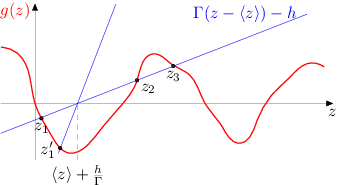
In the following we will consider the case where the velocity is sufficiently small $v\ll h$ . The positions where $\partial_{t}z=0$ follow from the intersection of $g(z)$ with the straight line $\Gamma(z-vt)-h$ which moves to the right with velocity $v$ (cf. Fig. 1). For sufficiently small $\Gamma$ and smooth $g(z)$ there are in general $2n+1$ intersections which we denote by $z_{1}<z_{2}<z_{3}<\ldots$ . For $z<z_{2}$ , $z$ is driven towards $z_{1}$ , for $z_{2}<z<z_{4}$ it is driven towards $z_{3}$ etc. If the particle starts with an arbitrary initial value, it will first develop towards the closest stable fixed point of (9), where the particle velocity is small. Let us assume this is $z_{1}$ . The force free point $z_{1}$ will then change according to $z_{1}(t)=vt+h/\Gamma+g(z_{1})/\Gamma$ . Eventually, the intersection point $z_{1}(t)$ merges with $z_{2}(t)$ and then disappears. In this case $z(t)$ will grow sufficiently fast until it reaches $z_{3}(t)$ and the process repeats if we replace $z_{n}\to z_{n-2}$ . Thus, the motion of the particle is jerky: periods of slow motion with velocity $v$ are intermitted by fast periods where the particle is driven towards a new stable fixed point. Below, we will analyse this process in detail.

III.1 The general picture

A first overview results from considering some limiting cases.

(i) For large but finite $\Gamma$ we can apply perturbation theory. To lowest non-trivial order one obtains for the mean velocity (a short derivation of this expression can be found in appendix C)

v=h+\int_{0}^{\infty}dt\,e^{-\Gamma t}\Delta^{\prime}(vt)\,.

(10)

The depinning threshold $h_{p,\pm}$ for $h\lessgtr 0$ follows from taking the limit $v\to\pm 0$ , $h\to\pm h_{p}\pm 0$

h_{p,\pm}\equiv-\lim\limits_{\varepsilon\to 0}\Gamma^{-1}\Delta^{\prime}(\pm\varepsilon).

(11)

Thus, the force correlator has to have a cusp singularity to produce a finite threshold. If there is no cusp, perturbation theory in $\Gamma^{-1}$ signals the absence of a depinning threshold. This argument applies however only to the region where perturbation theory is applicable, i.e. for $\Gamma\gg 1$ . This perturbative result is in accordance with our numerical analysis, as is shown in Fig. 2.

As has been mentioned in the introduction, a cusp singularity in the correlator emerges as a fixed point solution of the functional renormalization group (FRG) flow in $4-\epsilon$ dimensions and describes the effective randomness on scales larger than the Larkin length. This leads to the existence of a depinning threshold in all dimensions $d<4$ . Of course, in the framework of the mean field approximation an FRG study is senseless and a correlator with a cusp singularity has to be included manually. Nevertheless, as we already see here, in many aspects the assumption of a correlator with a cusp gives different results compared to a smooth correlator. Incidentally, Narayan and Fisher [9, 31] have used the mean field solution for cusped disorder to expand around in order to work out the critical behaviour of $4-\epsilon$ -dimensional systems.

(ii) Finally, we consider the case $\Gamma\ll 1$ . For $\Gamma=0$ the equation of motion (8) can be integrated

\int_{0}^{z}\frac{dz^{\prime}}{h+g(z^{\prime})}=t.

(12)

To calculate the integral we assume that $h>0$ and $h+g(0)>0$ . Then for small $z$ the lefthand side is positive and hence $t$ as well, so the velocity is finite. However, since $g(z)$ is unbounded there is a value $z_{1}$ at which the denominator vanishes. The integral is then dominated by the integration in the vicinity of $z_{1}$ Thus if $z$ approaches $z_{1}$ the time scale $t$ diverges and the velocity vanishes, the particle is pinned at $z=z_{1}$ . The same argument works for $h<0$ .

III.2 Static solution

One special class of solutions to the equation of motion (8) are the static solutions $z_{s}$ with $\partial_{t}z_{s}\equiv 0$ . Here, we are going to analyse under which circumstances such solutions can exist [32].

From the equation of motion Eq. (8) it is clear that

\Gamma\left(z_{s}-\langle z\rangle\right)-h=g(z_{s})

(13)

must be obeyed, i.e. the system has to be located at force-free positions.

Besides Eq. (13), one has to take into account that the self-consistency condition

h=-\langle g(z_{s})\rangle,

(14)

which follows from averaging (13) holds. The maximal value on the righthand side of (14) is realised, if $z_{s}\equiv z_{1}$ . Thus,

\displaystyle h_{p}=-\left\langle g(z_{1})\right\rangle

(15)

is a critical field strength, above which no static solutions are possible. Conversely, we can conclude that close to depinning all particles are localised at the leftmost force free points.

Let us now apply this argument to the case $\Gamma\gg 1$ . For a smooth potential as depicted in Fig. 1 there is typically only one solution $z_{1}^{\prime}$ . For this single solution, $g(z_{1}^{\prime})$ can be positive or negative with equal probability. Thus, a pinned solution obeying $h=-\left\langle g(z_{1}^{\prime})\right\rangle$ does not exist apart from the case $h=0$ . Hence, in this case the interface is never pinned, in agreement with our result from perturbation theory. The situation is different in the case when the random force exhibits infinite slopes as is shown in Fig. 3. Then, due to the discontinuities there are in general several solutions $z_{i}$ for any value of $\Gamma$ from which the leftmost ones dominate the behavior in the neighborhood of the depinning threshold. Of course, the larger the value of $\Gamma$ the smaller is the fraction of disorder realisations which allow for more than one force free solution. Thus, for large $\Gamma$ , the depinning threshold is diminished but finite. The presence of infinite slopes is a special feature of disorder forces, the correlator of which has a cusp singularity at the origin. A detailed analysis of the cusped disorder, as is sketched in Fig. 3 is presented in App. D, where we discuss how such a class of disorder forces can be realised and derive the correlator explicitly.

To test these predictions, we have solved equation (8) numerically. The depinning threshold $h_{p}$ is plotted in Fig. 2 as a function of $\Gamma$ . It is clearly seen that the threshold increases with $\Gamma^{-1}$ , it vanishes for $\Gamma>\Gamma_{c}$ for smooth random force correlations. For cusp correlations $\Gamma_{c}\to\infty$ . These findings support the results from perturbation theory.

III.3 Scaling behaviour above depinning

Now, we consider the behaviour slightly above the depinning threshold $h\gtrsim h_{p}$ , when $\left\langle z\right\rangle=vt$ but $v\ll 1$ . Our goal is to work out the scaling exponent $\beta$ for the sliding velocity $v$ , which we anticipate to vanish as a power law

\displaystyle v\sim(h-h_{p})^{\beta}.

(16)

To this aim, we solve the equation of motion in an approximate manner. As the velocity of the interface is small, $v\ll 1$ , we can also expect that $\partial_{t}z\ll 1$ for most of the time. Thus, $z(t)$ follows essentially from the vanishing of the righthand side of (9), which means that $z(t)$ stays close to the leftmost fixed point $z_{1}(t)$ . Since the disorder averaged position $\left\langle z\right\rangle$ is in motion, we have to keep in mind, that the root of the straight line in Figs. 1 and 3 is now moving relative to $g(z)$ . The intersection point $z_{1}(t)$ satisfies the relation

z_{1}(t)=vt+\Gamma^{-1}(h+g(z_{1}(t))).

(17)

Without loss of generality, we restrict ourselves to $v>0$ , so $z_{1}(t)$ moves now to the right. In this part of the motion, $z_{1}$ changes slowly (of order $v$ ). Eventually, $z_{1}$ merges with $z_{2}$ . Let us assume that this happens at $t=0$ . For further reference we denote

\displaystyle z_{0}\equiv z_{1}(0-)=z_{2}(0-).

(18)

For $t>0$ , these two solutions disappear and the intersection point $z_{3}(0-)$ becomes the new leftmost intersection point, i.e. $z_{3}(0-)\to z_{1}(0+)$ , so effectively $z_{1}$ jumps instantaneously. Thus, at $t>0$ , the position $z(t)$ is not any more close to a force free position and therefore it moves faster to approach the new intersection point $z_{1}(t)$ . The idea is now, that the mean velocity $v$ is mainly determined by those disorder realisations, which move fast. In order to determine the scaling exponent $\beta$ of $v$ , it is thus our task to work out a quantitative description of the motion of a particle in a certain disorder realisation during a period of time between two collapses of force-free points. The temporal distance between two jumps of the leftmost force-free position is approximately given by

\displaystyle T=v^{-1},

(19)

because this is the time needed to travel through a correlated region of the disorder (which is of length 1). We denote the distance to the new leftmost intersection point $z_{1}(t)$ by

\displaystyle\theta(t)=z(t)-z_{1}(t).

(20)

Note, that by definition $\theta(t)$ is negative. Now, Eq. (17) yields the identity

	$\displaystyle 0$	$\displaystyle=\langle z(t)-vt\rangle={1\over T}\int\limits_{0}^{T}dt\>\langle z_{1}(t)+\theta(t)-vt\rangle$
		$\displaystyle={1\over T}\int\limits_{0}^{T}dt\>\langle\Gamma^{-1}h+\Gamma^{-1}g(z_{1})+\theta(t)\rangle.$		(21)

Using Eq. (15), we obtain from (21)

\displaystyle{h-h_{p}\over\Gamma}=-{1\over T}\int\limits_{0}^{T}dt\>\left\langle\theta(t)\right\rangle.

(22)

The integral on the righthand side of (22) depends on the velocity. But, in order to use Eq. (22) to determine the scaling exponent, we have to describe the interface motion for $t>0$ , i.e. in the region of the fast motion between the previous and the new force free position. We are going to do this separately for the two types of disorder considered in this paper.

III.3.1 Disorder with a smooth correlator

The motion of the interface position after the collapse of the two leftmost force-free points is best analysed in several steps. First of all, we note that at $t=0$ when $z_{1}$ and $z_{2}$ merge, the relation

\displaystyle\Gamma=g^{\prime}(z_{0})

(23)

holds. For $t\gtrsim 0$ , we can expect that $z(t)$ is still close to $z_{0}$ , so we can expand (9) around $z_{0}$ . Writing

\displaystyle\zeta(t)=z(t)-z_{0}

(24)

and using (23), we obtain

\displaystyle\partial_{t}\zeta=\Gamma vt+{g^{\prime\prime}(z_{0})\over 2}\zeta^{2}+O(\zeta^{3}),\quad\zeta(0)=0.

(25)

For small $\zeta$ , we can neglect the second term on the righthand side and obtain

\displaystyle\zeta(t)\approx{\Gamma vt^{2}/2}.

(26)

On time scales $t\geq t_{0}=2[\Gamma vg^{\prime\prime}(z_{0})]^{-{1\over 3}}$ the second term on the righthand side of (25) dominates the time evolution and we obtain

\displaystyle\zeta(t)

\displaystyle\approx{2\over g^{\prime\prime}(z_{0})(t_{d}-t)},\quad t_{d}={3\over 2}t_{0}.

(27)

Clearly, this result can only be used until a time

\displaystyle t_{1}\simeq t_{d}-{2\over g^{\prime\prime}(z_{0})},

(28)

for which $\zeta(t_{1})\lesssim 1$ since we made an expansion in $\zeta$ . It shows, however, that for $t_{0}\lesssim t\lesssim t_{1}$ the coordinate $z$ increases rapidly until it comes close to the new leftmost minimum $z_{1}(t)$ . For $t>t_{1}$ , $\theta(t)$ is already close to zero and therefore gives only higher order contributions to the righthand side of Eq. (22).

The motion in between two jumps is sketched in Fig. 4

Now, we are going to evaluate the integral over $\theta(t)$ that occurs in Eq. (22). The equations (20) and (24) relate $\theta(t)$ and $\zeta(t)$

\displaystyle\theta(t)=\zeta(t)+z_{0}-z_{1}(t).

(29)

The time dependence of $z_{1}(t)$ can be estimated from Eq. (17) as

	$\displaystyle\partial_{t}z_{1}(t)$	$\displaystyle=v+\Gamma^{-1}g^{\prime}(z_{1}(t))\partial_{t}z_{1}(t)$
	$\displaystyle\Rightarrow\>\partial_{t}z_{1}(t)$	$\displaystyle={\Gamma v\over\Gamma-g^{\prime}(z_{1}(t))}={\Gamma v\over\Upsilon}+O(v^{2}),$		(30)

where we have introduced $\Upsilon=[\Gamma-g^{\prime}(z_{1}(0+))]$ for notational convenience. Since $z_{1}(0+)$ is a stable fixed point, we have $\Upsilon>0$ . Using

\displaystyle z_{0}-z_{1}(t)\simeq\theta(0)-{\Gamma v\over\Upsilon}t,

(31)

we obtain

$\displaystyle\int\limits_{0}^{t_{0}}dt\,\theta(t)=$	$\displaystyle\int\limits_{0}^{t_{0}}dt\,\left[\zeta(t)+\theta(0)-{\Gamma v\over\Upsilon}t\right]$
$\displaystyle=$	$\displaystyle{\Gamma vt_{0}^{3}\over 6}+t_{0}\theta(0)-{\Gamma v\over\Upsilon}{t_{0}^{2}\over 2}$
$\displaystyle=$	$\displaystyle 2v^{-{1\over 3}}\theta(0)[\Gamma g^{\prime\prime}(z_{0})]^{-{1\over 3}}+O(1).$	(32)

Further, for $t_{0}<t<t_{1}$ , we have

$\displaystyle\int\limits_{t_{0}}^{t_{1}}dt\,\theta(t)=$	$\displaystyle\int\limits_{t_{0}}^{t_{1}}dt\,\left[\zeta(t)+\theta(0)-{\Gamma v\over\Upsilon}t\right]$
$\displaystyle=$	$\displaystyle{2\over g^{\prime\prime}(z_{0})}\ln{t_{d}-t_{1}\over t_{d}-t_{0}}+\theta(0)(t_{1}-t_{0})-$
	$\displaystyle{\Gamma v\over\Upsilon}{t_{1}^{2}-t_{0}^{2}\over 2}$
$\displaystyle=$	$\displaystyle v^{-{1\over 3}}\theta(0)[\Gamma g^{\prime\prime}(z_{0})]^{-{1\over 3}}+O(\ln v).$	(33)

As we have already said, the integral over the remaining time interval $[t_{1};T]$ contributes to $O(1)$ only. Thus, up to orders $O(v\ln v)$ , from (32) and (33) the expression on the righthand side of Eq. (22) follows as

\displaystyle{1\over T}\int\limits_{0}^{T}dt\>

\displaystyle\langle\theta(t)\rangle\simeq-v^{2\over 3}3\left\langle|\theta(0)|[\Gamma g^{\prime\prime}(z_{0})]^{-{1\over 3}}\right\rangle.

(34)

From (22) and (34), we obtain therefore

v\sim{(h-h_{p})^{3/2}\over\Gamma},

(35)

i.e. $\beta=3/2$ .

III.3.2 Disorder with a cusped correlator

As we have mentioned before, if $\Delta(z)$ has a cusp singularity, the typical disorder force realisation exhibits discontinuous jumps, as is depicted in Fig. 3. A moment reflection shows, that a merging of two force free solutions $z_{1}$ and $z_{2}$ is only possible at such a discontinuity of the force field. The requirement, that $z_{1}$ is a stable fixed point entails that such a discontinuity is given by an upward jump in the force field. For the calculation we have to distinguish several cases.

Case 1: In this case we assume, that the next stable intersection point occurs before the next discontinuity. Then, we have the inequality (cf. Fig. 5)

\displaystyle\Gamma>g^{\prime}(z_{0}+).

(36)

It turns out that we have to solve the equation of motion in two time regimes. First, close to $t=0$ , $z(t)$ is in the vicinity of $z_{0}$ and we consider again the equation for

\displaystyle\zeta(t)=z(t)-z_{0}.

(37)

Now, since the merging of two fixed points occurs at the discontinuities of the potential, Eq. (23) is not meaningful, but instead $z_{0}$ fulfills the equation

\Gamma z_{0}=g(z_{0}-)+h.

(38)

Using Eq. (38), it is easy to see that the equation of motion for $\zeta(t)$ takes the form

	$\displaystyle\partial_{t}\zeta(t)$	$\displaystyle\approx\Gamma(vt-z_{0})+g(z_{0}+)+(g^{\prime}(z_{0}+)-\Gamma)\zeta+h$
		$\displaystyle=\Gamma vt-(\Gamma-g^{\prime}(z_{0}+))\zeta(t)+\delta g.$		(39)

Here, $\delta g=g(z_{0}+)-g(z_{0}-)$ denotes the jump of $g(z)$ which is of order one. Integration of (39) gives for short times $t\gtrsim 0$

\zeta(t)\approx{\delta}g\,t.

(40)

This result is approximately correct for $t<t_{0}$ with

\displaystyle t_{0}=(\Gamma-g^{\prime}(z_{0}+))^{-1}.

(41)

Note, that due to (36) the time $t_{0}$ is always finite and positive, in fact generically of order $O(1)$ . For $t>t_{0}$ , also the term in Eq. (39) proportional to $\zeta(t)$ becomes relevant. Now, $z_{0}+\zeta(t_{0})$ has to be compared with $z_{1}(0+)$ which is the new leftmost intersection point for $t>0$ . From (17) we deduce that $z_{1}(0+)$ fulfills the equation

\Gamma z_{1}(0+)\approx h+g(z_{0}+)+g^{\prime}(z_{0}+)(z_{1}(0+)-z_{0}),

(42)

from which we obtain

	$\displaystyle z_{1}(0+)$	$\displaystyle\approx\frac{h+g(z_{0}+)-g^{\prime}(z_{0}+)z_{0}}{\Gamma-g^{\prime}(z_{0}+)}$
		$\displaystyle={[\Gamma-g^{\prime}(z_{0}+)]z_{0}+\delta g\over\Gamma-g^{\prime}(z_{0}+)}=\zeta(t_{0})+z_{0}=z(t_{0}).$		(43)

In the second step, we have replaced $h$ using Eq. (38). Thus, after the time $t_{0}$ the particle has reached already the new intersection point $z_{1}$ .

To determine the exponent $\beta$ , we want to employ equation (22) again. For $t\leq t_{0}$ , the relevant function $\theta(t)$ as has been obtained so far reads

\displaystyle\theta(t)=z_{0}-z_{1}(t)+\zeta(t)\approx z_{0}-z_{1}(t)+\delta gt.

(44)

To approximate the time dependence of $z_{1}(t)$ , we expand $z_{1}(t)$ around $z_{1}(0+)$ and get

\displaystyle z_{1}(t)\simeq z_{1}(0+)+\dot{z}_{1}(0)t.

(45)

Here, $\dot{z}_{1}(0)$ can be deduced from the defining equation (17), it follows as $\dot{z}_{1}(0)=\Gamma vt_{1}$ with

\displaystyle t_{1}=(\Gamma-g^{\prime}(z_{1}(0)))^{-1}.

(46)

Thus, in the regime where $\theta(t)$ changes fast, i.e. for $t\leq t_{0}$ , we can write

\displaystyle\theta(t)\approx z_{0}-z_{1}(t)+\zeta(t)\simeq\delta g(t-t_{0})-\Gamma vt_{1}\,t.

(47)

This shows, that for $t>t_{0}$ , $\theta(t)=O(v)$ . However, the time scale $t_{0}$ is of the order $O(1)$ , and is thus small compared to $T$ , $t_{0}\ll T$ . Therefore, it is important to carefully analyse the function $\theta(t)$ also for $t>t_{0}$ . For $t>t_{0}$ we expand around $z_{1}(t)$ and the approximated equation of motion reads

\displaystyle\partial_{t}z

\displaystyle\simeq\Gamma(vt-z)+g(z_{1})+g^{\prime}(z_{1})(z-z_{1})+h=-{1\over t_{1}}\theta(t),

(48)

where $t_{1}$ is defined in (46). Then, using (17) and (20), we find

\displaystyle\partial_{t}\theta

\displaystyle\simeq-{1\over t_{1}}\theta(t)-\Gamma vt_{1}.

(49)

The solution to this equation, matching with equation (47) gives

\displaystyle\theta(t)\approx-\Gamma vt_{1}^{2}+\Gamma vt_{1}(t_{1}-t_{0})\,e^{-(t-t_{0})/t_{1}}.

(50)

The motion $z(t)$ in between two jumps is sketched in Fig. 6

Now, we can determine $\beta$ using equation (22). In calculating

\displaystyle-{1\over T}\int\limits_{0}^{T}dt\,\left\langle\theta(t)\right\rangle\simeq v\left\langle{\delta gt_{0}^{2}\over 2}+\Gamma t_{1}^{2}\right\rangle+O(v^{2}),

(51)

we have decomposed the integral into the intervals $0\ldots t_{0}$ and $t_{0}\ldots T$ , respectively. This gives

\displaystyle v

\displaystyle\sim{h-h_{p}\over\Gamma},

(52)

from which we conclude, that in the case of cusped disorder the velocity exponent is $\beta=1$ .

Case 2: Now, we have to discuss what can change if there is a discontinuity of $g(z)$ in between $z_{0}$ and $z_{1}(0+)$ . One possible scenario for this case is depicted in the right part of Fig. 5. We are going to discuss now, that our main result $\beta=1$ remains unchanged. Indeed, as can be concluded from our previous calculation, the essential point that lead to the exponent $\beta=1$ was the fact, that $z(t)$ approaches $z_{1}(0+)$ on a time scale $t_{0}$ which is of order $O(1)$ . Responsible for this is, that immediately after a collapse of the leftmost intersection point, the particle starts to move with a velocity of order $\delta g=O(1)$ . This remains unchanged. In Fig. 6 we have also sketched the motion when a discontinuity occurs in between $z_{0}$ and $z_{1}(0+)$ . The respective quantities in Fig. 6 carry a prime. The only effect of the discontinuity that is crossed at a time $t^{\prime}_{j}$ is a singularity of the velocity $\dot{z}^{\prime}(t)$ at $t=t^{\prime}_{j}$ . Therefore, the fundamental characteristics of the motion remain unchanged. Thus, in case of $k$ jumps of $g(z)$ the foregoing calculation remains basically unchanged, apart from the fact, that one should now decompose the motion in more parts: $[0;t_{j_{1}}]$ , $[t_{j_{1}};t_{j_{2}}]$ , …, $[t_{j_{k}};t_{0}]$ , $[t_{0};T]$ . Of course, this consideration changes the prefactor in Eq. (52), which is, however, anyway beyond our accuracy.

The two exponents $\beta=3/2$ for smooth and $\beta=1$ for cusped disorder are confirmed by our numerical solution as depicted in Fig. 7.

IV Finite Frequencies

In the finite frequency case, the disorder average over the solutions to the equation of motion (7) forms a hysteresis in the $v$ - $h$ -plane, as is illustrated in Fig. 8 for the two types of disorder considered here. The hystereses are invariant under the transformation $v\to-v$ and $h\to-h$ . This can be explained directly using the equation of motion (7) and a statistical inversion symmetry. Taking the disorder average of (7) yields

\displaystyle\partial_{t}\left\langle z\right\rangle=v=h\cos\omega t+\left\langle g(z(t))\right\rangle.

(53)

It is easy to see, that the aforementioned symmetry under $v\to-v$ and $h\to-h$ holds true if the probability density $P(g)$ (cf. Eq. (5)) obeys $P(g)=P(\hat{g})$ where $\hat{g}(z)=-g(-z)$ . This is obviously the case for our assumption of Gaussian disorder (cf. Sec. II).

IV.1 Qualitative discussion of the motion

To understand the shape of the hysteresis, we consider the motion of a particle for half of a period for the case $h\gg h_{p}$ and small frequency $\omega\ll\Gamma$ . We start at a time $t=0$ , when $h(0)=-h_{p}$ and the field increases. Then, we can expect each particle to be located close to the rightmost force free point, i.e. the rightmost solution of

\Gamma\left(z_{f}(t)-\left\langle z\right\rangle(t)\right)-h(t)=g(z_{f}(t)).

(54)

In Fig. 9 it is illustrated, that due to the change of the driving field towards larger values, the root of the straight line, given by

\displaystyle z_{r}\equiv\left\langle z\right\rangle(t)+h(t)/\Gamma

(55)

moves with a velocity

\displaystyle\dot{z}_{r}=v(t)+{\dot{h}(t)\over\Gamma}.

(56)

Since $\dot{h}(t)>0$ , this velocity is positive although the value of the field is still negative. Therefore, also the intersection point $z_{f}(t)$ to which the particle is connected, moves to the right. This fact is observed in the hysteresis loop, illustrated in Fig. 8.

Actually, this understanding allows to estimate the velocity in simple geometrical terms. Using the notation explained in Fig. 10, we have ${\delta g/\delta z_{f}}\simeq g^{\prime}(z_{f})$ and thus

\displaystyle\delta z_{r}-\delta z_{f}=-{\delta g\over\Gamma}=-{g^{\prime}(z_{f})\delta z_{f}\over\Gamma},

(57)

from which we conclude

\displaystyle\delta z_{r}={\Gamma-g^{\prime}(z_{f})\over\Gamma}\delta z_{f}.

(58)

Now, Eq. (56) yields

\displaystyle{\delta z_{r}\over\delta t}={\Gamma-g^{\prime}(z_{f})\over\Gamma}{\delta z_{f}\over\delta t}\simeq{\delta z_{f}\over\delta t}+{\dot{h}(t)\over\Gamma}.

(59)

Solving the last approximate equality for $\delta z_{f}/\delta t$ , we obtain

\displaystyle\dot{z}_{f}\simeq-\dot{h}/g^{\prime}(z_{f}).

(60)

During the motion of $z_{f}(t)$ , other intersection points to the left of $z_{f}(t)$ vanish, and new solutions to the right emerge. Finally, when $h(t_{1})\approx h_{p}$ , $z_{f}(t_{1})$ has become the leftmost intersection point. From approximately this time on it happens, that occasionally in some disorder realisations $z_{f}(t)$ merges with an unstable fixed point and vanishes, so that the particle moves fast in order to catch up with the new leftmost force free point. This procedure has already been discussed earlier in Sec. III. Since the velocity of a particle is given by the difference between $g(z)$ and the straight line $\Gamma(z-\left\langle z\right\rangle)-h$ , it must fall back behind the leftmost intersection point to speed up. This can only happen due to the disappearance of force free points. Thus, the velocity grows slowly because after each jump the particle moves fast and thus approaches again the new intersection point. On the other hand, by virtue of Eq. (56), the larger $v(t)$ the faster $z_{r}(t)$ and thus also the faster the intersection points move. This leads to a positive feedback and entails a strong slope when the velocity is large enough such that the particle is no longer able to approach a force free point before the next jump sets in. Finally, far above $h_{p}$ the particle is depinned. After the driving force has reached its maximum it decreases. Note that the root of the straight line $z_{r}$ has now a velocity smaller than $v(t)$ , because $\dot{h}$ is negative. Therefore, the particle position $z(t)$ approaches $z_{r}(t)$ and slows down. Hence, $\dot{h}$ is a measure also for the decrease of $v(t)$ . On approaching $h_{p}$ from above, all particles are still depinned and hence far enough behind the leftmost intersection point, so that the latter has only little influence on the motion of the particle and the velocity decays with the same slope all the time. Only when $v(t)$ has passed below $\dot{h}/\Gamma$ , $z_{r}$ moves in the negative direction and thus the intersection points as well. This means, that the leftmost intersection point approaches the particle before it is pinned. After the particle is a little to the right of the leftmost force free position, which happens about when $h(t)\approx h_{p}$ , the velocity is negative. Now, the same procedure starts in the other direction.

As $\omega\to 0$ , the hystereses approach the depinning curve that has been discussed in the previous chapter. In the following, we are going to take a closer look on the details of this limiting process.

IV.2 Velocity exponents

First, we want to work out, how

\displaystyle v_{h_{0}}\equiv|v(h=0)|

(61)

approaches zero as $\omega\to 0$ . As we have explained in Sec. IV.1, the particle in each disorder realisation stays close to a force-free point, that we have agreed to label $z_{f}(t)$ . The velocity $\partial_{t}z$ of the particle is now determined solely by the velocity of the force free position $z_{f}$ that we are now going to calculate in a more accurate way than our estimate from Eq. (60). Let $t_{0}$ be the point in time, at which $h(t_{0})=0$ . On time scales that are small compared to the period $\omega^{-1}$ , we can linearly expand the driving field around $t_{0}$

\displaystyle h(t)\simeq-h\omega(t-t_{0}).

(62)

Further, we want to expand (54) around $z_{f}(t_{0})$ . For small distances in time we can neglect possible changes in the velocity and write

\displaystyle z_{f}(t)\simeq z_{f}(t_{0})+v_{f}(t-t_{0}),

(63)

where $v_{f}=\partial_{t}z_{f}$ is a shorthand notation. Using (62) as well as $\left\langle z\right\rangle(t)\simeq\left\langle z\right\rangle(t_{0})-v_{h_{0}}(t-t_{0})$ , we have

$\displaystyle 0=$	$\displaystyle\Gamma\big[z_{f}(t_{0})+v_{f}(t-t_{0})-\left\langle z\right\rangle(t_{0})+v_{h_{0}}(t-t_{0})\big]+$
	$\displaystyle h\omega(t-t_{0})-g(z_{f}(t_{0}))-g^{\prime}(z_{f}(t_{0}))v_{f}(t-t_{0})$	(64)
$\displaystyle=$	$\displaystyle(t-t_{0})\big[\Gamma(v_{f}+v_{h_{0}})+h\omega-v_{f}g^{\prime}(z_{f}(t_{0}))\big]$	(65)

Since this should hold for small but finite $|t-t_{0}|$ , the expression in the rectangular brackets has to vanish. Solving (65) for $v_{f}$ , taking the disorder average and using the self-consistency condition $\left\langle v_{f}\right\rangle=-v_{h_{0}}$ finally yields

\displaystyle v_{h_{0}}=-{h\omega\over\Gamma-\left\langle[\Gamma-g^{\prime}(z_{f}(t_{0}))]^{-1}\right\rangle^{-1}}.

(66)

Since $g^{\prime}(z_{f}(t_{0}))<0$ , which expresses the reasonable assumption that $z_{f}$ is a stable force free position, $v_{h_{0}}$ is indeed positive, which must be the case by its definition (61). Note, that our derivation so far does not make any assumption about the disorder correlator, whence it holds for cusped as well as for smooth disorder. In conclusion, for $\omega\to 0$ the width of the hysteresis at $h=0$ behaves as $v_{h_{0}}\sim\omega^{\kappa}$ with $\kappa=1$ for either kind of disorder. This exponent is verified by our numerical analysis, cf. figure 11.

Another interesting quantity to look at is

\displaystyle v_{h_{p}}\equiv|v(h=h_{p})|,

(67)

of which we want to work out the limiting behaviour for $\omega\to 0$ . As $h(t)$ increases further from $0$ towards $h_{p}$ , more and more of the force free points $z_{f}$ , which the true positions in the disorder realisations are following, become the rightmost ones, so that occasionally jumps occur. On closely approaching $h(t)=h_{p}$ the dominant contribution originates from these jumps, which severely affects the exponent, so that $v_{h_{p}}\sim\omega^{\mu}$ with $\mu\simeq 1/2$ , as can be inferred from our numerical analysis, shown in figure 12.

This exponent is again independent of the shape of the disorder correlator at the origin (smooth or cusped). An analytical derivation of this exponent is much more complicated than it was the case for $\kappa$ and in fact we did not find a rigorous prediction. For the finite dimensional case in $4-\epsilon$ dimensions, the exponent $\mu$ has been found as $\mu=\beta/(\nu z)$ , where $\nu$ denotes the correlation length exponent and $z$ the dynamical exponent [21].

IV.3 The area of the hysteresis loop

Next, we want to investigate the limiting behaviour of the hysteresis area. The physical meaning of the loop area can be concluded from the energy balance of an overdamped system. For the change of the disorder averaged potential energy in time, we find (cf. App. E)

\displaystyle\partial_{t}\left\langle E\right\rangle=h(t)v(t)-\left\langle(\partial_{t}z)^{2}\right\rangle.

(68)

Here, $h(t)v(t)$ measures the energy gain through the work per unit time that is done by the external field and $\left\langle(\partial_{t}z)^{2}\right\rangle$ measures the energy loss per unit time due to dissipation. The area of the hysteresis loop is determined via

\displaystyle A_{\text{hyst}}(\omega)

\displaystyle=\oint v(t)\,dh=\int\limits_{0}^{T}v(t)\dot{h}(t)\,dt.

(69)

This means, the loop area denotes the integrated change in work per unit time due to the change of the external field.

Note, that in the case of a double hysteresis (which occurs for large $h$ , when the motion of the system over one period extends on average over more than one valley of the disorder potential), the area is given by the area of the inner hysteresis minus the area of the two outer hystereses (cf. Fig. 8). Formally, this is because the inner hysteresis is traversed clockwise, whereas the outer loops are passed through counter-clockwise. Physically, this can be understood as follows. Starting from $h=0$ at the branch of increasing $h(t)$ , the external field works against the potential gradient due to elastic energy and disorder. On going over into the regime of the outer loops, sliding behaviour sets in and thus the potential energy, stored so far in the system, adds to the work done by the external field. This fact is responsible for the steep slope at the beginning of the outer loop. In other words, during the period in the outer loops, the external field does not any more work against a potential gradient, but together with the potential energy the system is accelerated.

To work out the hysteresis loop area as $\omega\to 0$ , we distinguish three cases.

(a) $h\ll h_{p}$ . In this situation, the hysteresis consists of a single loop. The outer loops, visible in Fig. 8, are absent. We expect the loop area to be given by $A_{\text{hyst}}\approx v_{h_{0}}h\sim\omega^{\kappa}$ . Indeed, our numerical solution shows that the area of the hysteresis vanishes proportional to $\omega$ , independent of the type of disorder correlator, as shown in Fig. 13.

(b) $h=h_{p}$ . For this case, the hysteresis loop is still single (no double hysteresis) and the hysteresis area decreases with the frequency as $A_{\text{hyst}}\sim\omega^{0.82}$ (cf. Fig. 14), still independent of the disorder correlator.

(c) $h\gg h_{p}$ . Now, we face the situation of a double hysteresis and moreover, the behaviour of the hysteresis area as $\omega\to 0$ now depends on the shape of the disorder correlator. We find $A_{\text{hyst}}\sim\omega^{\alpha}$ with $\alpha\simeq 0.67\approx 2/3$ for cusped and $\alpha\simeq 0.75=3/4$ for smooth disorder. This is shown in figure 15.

So far, our results suggest that the scaling exponents are insensitive to the nature of the disorder correlator as long as the force amplitude does not exceed the threshold $h_{p}$ . These findings seem to milden the non-universality conclusion by Fisher [8], who considered the response of a charge density wave system to an ac force in addition to dc driving. He distinguished different distributions of the random amplitude (pinning strength) of the disorder potential in addition to a random phase, and found a strong dependence of the behaviour on the type of disorder both above and below threshold.

For large frequencies, the area of the hysteresis loop vanishes as well. Above a certain crossover frequency, which depends on $h$ , the motion of the particle is restricted to one minimum of the potential. Thus, for large enough frequencies we can approximate the potential by a harmonic one, such that the equation of motion for the disorder averaged position becomes

\displaystyle v(t)=h\,\cos\omega t-w\,z(t),

(70)

which has the solution

\displaystyle v(t)={w\omega h\over w^{2}+\omega^{2}}\left[-\sin\omega t+{\omega\over w}\cos\omega t\right].

(71)

Thus, using Eq. (69) we find for the hysteresis loop area

\displaystyle A_{\text{hyst}}(\omega)

\displaystyle=\int\limits_{0}^{T}v(t)\dot{h}(t)\,dt={w\omega^{2}h^{2}\over w^{2}+\omega^{2}}{\pi\over\omega}\sim\omega^{-1},

(72)

where the last expression gives the asymptotics for large $\omega$ .

The decay of the hysteresis loop area for large and small frequencies of the driving force requires the existence of a maximum. This maximum is found to be proportional to the resonance frequency of the typical disorder potential wells $\omega_{r}=\gamma u_{0}/\ell$ , which equals 1 in our units. The proportionality factor is of order unity, and is found different for small driving fields (single hysteresis) and large drivings (double hysteresis).

V Conclusions

For the mean-field theory of driven elastic manifolds in disordered systems, we have worked out the scaling behaviour of the velocity as a function of the dc-driving force close to depinning by extending Fisher’s [8] arguments for charge density waves. The scaling exponents are found to be different for disorder with smooth and cusped correlator. Our analytical findings are supported by a numerical treatment.

Furthermore, we have investigated the small-frequency behaviour of quantities that characterise the velocity hysteresis in case the system is exposed to an ac-driving. We found that the frequency scaling exponents of the remanent velocity $v_{h_{0}}$ and the velocity at the depinning field $v_{h_{p}}$ do not depend on the presence or absence of a cusp-singularity at the origin of the disorder correlator. This also holds for the frequency exponents of the hyteresis loop area as long as the amplitude of the driving does not exceed the depinning force $h_{p}$ . For force amplitudes above the depinning threshold, our numerical treatment yields different exponents for smooth and cusped correlators.

Acknowledgements.

For fruitful discussions we are grateful to G. M. Falco and A. A. Fedorenko. Moreover, we want to acknowledge financial support by Sonderforschungsbereich 608.

Appendix A Applicability of the mean field theory

Mean field theory is valid above the upper critical interface dimension $D_{c}$ , where the interface is not rough and there is no depinning transition for weak disorder. Below this critical dimensionality, the interface is soft enough to adapt to the random potential. Hence, it becomes rough and is pinned for small driving forces. An FRG analysis of the depinning transition shows, that the exponents become non-classical and the disorder correlator develops a cusp singularity [17]. The exponents can be expressed in terms of an $\epsilon$ -expansion, where $\epsilon=D_{c}-D$ , and the zeroth order $O(\epsilon^{0})$ is given by the critical exponents of mean-field theory with a cusped disorder correlator [31].

For systems with short range interaction it turns out that $D_{c}=4$ , so interface dimensionalities above $D_{c}$ seem to be a purely academic problem. There are, however, systems with long range forces for which the upper critical dimension $D_{c}$ is reduced. For example, for interfaces in systems with long range dipolar interaction it has been argued in Ref. [33] that the upper critical dimension decreases to $D_{c}=3$ . A further decrease of the critical dimension for the statics of interfaces is achieved for domain walls in ferroelectric materials with a piezo effect in the paraphase. An example for such a material is KDP. A peculiarity of such systems is that interfaces between different ferroelectric domains are allowed to be oriented along some distinguished orientations in the crystal only. This is because ferroelectric domain walls are at the same time ferroelastic domain walls which have to fulfill certain mechanical compatibility relations [34, 35]. Looking at the statics, one finds that in the presence of random field disorder the interface is not rough for $D\geq 2$ [36, 37]. In the following, we are going to take a look on the impact of these long range forces on the dynamical properties.

Firstly, we note that our model equation of motion (1) can be written in a more general fashion as

	$\displaystyle{1\over\gamma}\partial_{t}z({\boldsymbol{x}},t)=$	$\displaystyle u_{0}g({\boldsymbol{x}},z)+h(t)$
		$\displaystyle+\int d^{d}{\boldsymbol{x}}^{\prime}\,\Gamma_{\text{el}}({\boldsymbol{x}}-{\boldsymbol{x}}^{\prime})z({\boldsymbol{x}}^{\prime},t),$		(73)

where

\displaystyle\Gamma_{\text{el}}({\boldsymbol{x}})=\int_{{\boldsymbol{k}}}e^{i{\boldsymbol{k}}{\boldsymbol{x}}}\Gamma_{\text{el}}({\boldsymbol{k}}).

(74)

In (1) we assumed that only short range forces are present and hence

\displaystyle\Gamma_{\text{el}}({\boldsymbol{k}})=\Gamma_{0}k^{2}.

(75)

For the systems with long range forces, discussed above, the functional form of $\Gamma_{\text{el}}({\boldsymbol{k}})$ is different from (75). In systems with dipolar interactions, one finds [4]

\displaystyle\Gamma_{\text{el}}({\boldsymbol{k}})=\Gamma_{0}k^{2}+\lambda{k_{a}^{2}\over d-2}\left[(k\xi_{0})^{2-d}-1\right],

(76)

where $\lambda$ measures the strength of the dipolar interaction and $\xi_{0}$ is of the order of the lattice spacing. Here, $k_{a}$ is the component of ${\boldsymbol{k}}$ along the orientation of the dipoles. A further increase of the domain wall stiffness is achieved for domain walls in ferroelectric materials with a piezo effect in the paraphase. Integrating out the elastic degrees of freedom in such a (3d) system leads to an interface Hamiltonian of the form [36]

\displaystyle\Gamma_{\text{el}}({\boldsymbol{k}})=\Gamma_{0}k^{2}+\lambda{k_{a}^{2}\over k}+ck.

(77)

Here, $c$ is a constant that depends on the strength of the piezo coupling as well as on the elastic constants and $\lambda$ depends on the strength of the dipolar coupling, the piezo coupling coefficient and the elastic constants. Moreover, $k_{a}$ denotes the component of ${\boldsymbol{k}}$ in the direction of the polarisation.

In the following, we focus on the case of a dc-driving field $h(t)\equiv h$ . For the perturbative determination of the velocity, it turns out to be useful to go over to a co-moving frame $z({\boldsymbol{x}},t)=vt+\zeta({\boldsymbol{x}},t)$ . Expanding the correction $\zeta({\boldsymbol{x}},t)$ in a power series in $u_{0}$ ,

\displaystyle\zeta({\boldsymbol{x}},t)=\sum\limits_{n=0}^{\infty}u_{0}^{n}\zeta_{n}({\boldsymbol{x}},t),

(78)

one can solve Eq. (73) perturbatively by comparing equal orders of $u_{0}$ . Following the computation in Ref. [18] (which is similar to that presented in App. C below), we obtain a self-consistent perturbative expression for $v$ (the following equation corresponds to Eq. (29) in Ref. [18])

	$\displaystyle v-\gamma h$	$\displaystyle\simeq\int_{q}\int_{{\boldsymbol{k}}}{iu_{0}^{2}q\Delta_{q}\over\Gamma_{\text{el}}({\boldsymbol{k}})-i{vq\over\gamma}}$
		$\displaystyle=\int_{q}\int_{{\boldsymbol{k}}}{iq\Delta_{q}u_{0}^{2}(\Gamma_{\text{el}}({\boldsymbol{k}})+i{vq\over\gamma})\over[\Gamma_{\text{el}}({\boldsymbol{k}})]^{2}+{v^{2}q^{2}\over\gamma^{2}}}.$		(79)

Here, $\Delta_{q}$ denotes the Fourier transform of the disorder correlator defined in Eq. (6). For $v\to 0$ , our choice (75) for $\Gamma_{\text{el}}({\boldsymbol{k}})$ leads to a divergence of the integral in (79) when $D<4$ . The divergence stems from the contribution of small ${\boldsymbol{k}}$ . In contrast, for a model the elastic interaction of which assumes the form given by Eq. (77), the integral in Eq. (79) is convergent as long as $D>2$ and exhibits only a logarithmic divergence in $D=2$ . Thus, in such a system mean field results may apply for two-dimensional domain walls with small logarithmic corrections.

Appendix B Numerics

In this appendix, the details of our numerical methods shall be explained briefly. Numerically, we have solved the equation of motion (7) for 20000 different disorder configurations using the well established classical Euler method. Before embarking on the details of the procedure in the two cases of dc and ac driving, respectively, we want to explain how the different realisations of the disorder forces are achieved.

The random force associated to the smooth disorder correlator is generated by concatenating straight lines at distance 1. The values of the disorder force at the concatenation points are randomly chosen out of a bounded interval $[-m;m]$ . The bounds $m$ for this interval are determined such that the correlator fulfills $\Delta(0)=1$ . We found $m\simeq 2.1$ . Moreover, the position $s$ of the concatenation point closest to the origin $z=0$ has been determined randomly out of the interval $[-{1\over 2};{1\over 2}]$ . This method has already been used earlier by A. Glatz [38]. A sample configuration is depicted in Fig. 16.

To realise disorder forces with Gaussian statistics that are correlated with a cusp singularity at the origin, we have also used straight lines, the extension in $z$ -direction being again 1. In contrast to the former case, these lines are now concatenated discontinuously. The values of $g(z)$ at both endpoints of a segment are determined randomly from a bounded interval $[-m;m]$ . The size of this interval is again determined in such a way that the disorder correlator obeys $\Delta(0)=1$ with the same result of $m\simeq 2.1$ as before. Also the position $s\in[-{1\over 2};{1\over 2}]$ of the jump closest to $z=0$ is created randomly. An example for such a configuration is shown in Fig. 17. In App. D we discuss the latter generation technique in more detail and also derive the force correlator.

Moreover, we have verified numerically, that the assumed shapes for the disorder correlators are reflected by our two generation techniques. The result is shown in Fig. 18. As required, one correlator is smooth and the other shows a cusp singularity at the origin, perfectly in agreement with the analytic result (cf. Eq. (96) below). In both cases, the correlations decay to zero on a length scale $\ell\simeq 1$ .

To solve the equation of motion with a constant driving force for several values of $\Gamma$ and $h$ , we have chosen the initial condition $v(0)=0$ and $z(0)=0$ . The time steps are chosen to be of size $2^{-10}$ and we have simulated the equation of motion for $2^{14}$ such time steps. To avoid that our results are spoiled by transience effects, we have only taken into account the values of $v$ for the last $2^{10}$ time steps.

Our results that we have obtained for the ac driving case rely on the initial conditions $z(0)=0$ , $v(0)=h$ with $h(t)=h\,\cos\omega t$ . Before making any measurements we have been waiting for at least 2 periods for transience effects to diminish. The values for $v(h=0)$ and $v(h=h_{p})$ are measured then over 3 periods with 2 datapoints per period.

In all cases where we have numerically determined important exponents, we have given error estimates. These include the statistical deviations.

Appendix C Perturbation theory

To set up the perturbation expansion for our equation of motion (8)

\displaystyle\partial_{t}z=\Gamma(\left\langle z\right\rangle-z)+h+g(z),

(80)

we write $z(t)=\left\langle z(t)\right\rangle+\zeta(t)$ , $\partial_{t}z=v+\partial_{t}\zeta$ , so that $\left\langle\zeta\right\rangle=0$ . This yields two coupled differential equations

	$\displaystyle v$	$\displaystyle=h+\left\langle g(\left\langle z\right\rangle+\zeta)\right\rangle$		(81)
	$\displaystyle(\partial_{t}+\Gamma)\zeta$	$\displaystyle=g(\left\langle z\right\rangle+\zeta)-\left\langle g(\left\langle z\right\rangle+\zeta)\right\rangle.$		(82)

The differential operator on the left hand side of (82) has the fundamental solution

	$\displaystyle(\partial_{t}+\Gamma)G(t)$	$\displaystyle=\delta(t),$		(83)
	$\displaystyle G(t)$	$\displaystyle=\Theta(t)\,e^{-\Gamma t}.$		(84)

Now, for large enough $\Gamma$ , we can expect $\zeta(t)\ll 1$ and perform a Taylor expansion of the disorder force

\displaystyle g(\left\langle z\right\rangle+\zeta)

\displaystyle=\sum\limits_{n=0}^{\infty}{g^{(n)}(\left\langle z\right\rangle)\over n!}\zeta^{n}.

(85)

Thus, (81) gives us

	$\displaystyle v$	$\displaystyle=h+\left\langle g(\left\langle z\right\rangle)+g^{\prime}(\left\langle z\right\rangle)\zeta+\ldots\right\rangle$
		$\displaystyle=h+\left\langle g^{\prime}(\left\langle z\right\rangle)\zeta(t)+\ldots\right\rangle$		(86)

For $\zeta(t)$ , we use the lowest order result from the iteration (82) combined with (85)

	$\displaystyle\zeta(t)$	$\displaystyle=\int\limits_{t_{0}}^{\infty}dt^{\prime}\,G(t-t^{\prime})\left[g(\left\langle z(t^{\prime})\right\rangle+\zeta)-\left\langle g(\left\langle z(t^{\prime})\right\rangle+\zeta)\right\rangle\right]$
		$\displaystyle=\int\limits_{t_{0}}^{t}dt^{\prime}\,e^{-\Gamma(t-t^{\prime})}\left[g(\left\langle z(t^{\prime})\right\rangle)+\ldots\right],$		(87)

where $t_{0}$ is the time at which we fix our initial value problem. Sending $t_{0}\to-\infty$ , we obtain

	$\displaystyle v$	$\displaystyle=h+\int\limits_{-\infty}^{t}dt^{\prime}\,e^{-\Gamma(t-t^{\prime})}\left\langle g^{\prime}(\left\langle z(t)\right\rangle)g(\left\langle z(t^{\prime})\right\rangle)\right\rangle+\ldots$
		$\displaystyle=h+\int\limits_{-\infty}^{t}dt^{\prime}\,e^{-\Gamma(t-t^{\prime})}\Delta^{\prime}[\left\langle z(t)\right\rangle-\left\langle z(t^{\prime})\right\rangle].$		(88)

A change of the integration variable $t^{\prime}\to t-t^{\prime}$ and noting, that $\left\langle z(t)\right\rangle=vt$ then immediately yields the result given by (10).

Appendix D Generation of disorder forces with a cusped correlator

In this appendix, we propose a generation technique for disorder forces with a cusp singularity in the correlator and prove, that the cusp is indeed present. The method described here has also been employed in our numerical analysis, cf. App. B.

Consider a function $g(z)$ , that is constructed as follows. We decompose the $z$ -axis in intervals $I_{i}=[z_{i};z_{i+1}]$ of length $1$ . The starting point of each interval $I_{i}$ is given by

\displaystyle z_{i}=i+s,

(89)

where $i$ is an integer (the label for the interval) and $s$ is a random number, uniformly distributed in the interval $[-{1\over 2};{1\over 2}]$ . The function $g(z)$ shall now be given piecewise for each interval $I_{i}$ as a straight line. This line is determined by the left boundary point $(z_{i},\alpha_{i})$ and the right boundary point $(z_{i+1},\beta_{i})$ , where $\alpha_{i}$ and $\beta_{i}$ are chosen randomly out of a bounded interval $[-m;m]$ . The value of $m$ will be determined further down in such a way, that $\Delta(0)=1$ .

In more mathematical terms, a specific realisation of the function $g(z)$ is specified by the random number $s\in[-{1\over 2}:{1\over 2}]$ and two stets of boundary values $\{\alpha_{i}\}$ and $\{\beta_{i}\}$ . Using the indicator function $K(z;z_{i},z_{i+1})$ for each interval $I_{i}$ , defined by

\displaystyle K(z;z_{i},z_{i+1})=\left\{\begin{matrix}1&\quad z_{i}\leq z<z_{i+1}\\ 0&\quad\text{otherwise}\end{matrix}\right.,

(90)

the function $g(z)$ is explicitly given by

	$\displaystyle g(z,[s;\{\alpha_{i}\};$	$\displaystyle\{\beta_{i}\}])=\sum_{i}K(z;z_{i},z_{i+1})$
		$\displaystyle\times\big[(\beta_{i}-\alpha_{i})(z-i-s)+\alpha_{i}\big].$		(91)

Examples for typical configurations of $g(z)$ are depicted in the Figs. 3 and 17. An illustration for a single segment is sketched in Fig. 19. In the following, we are going to show, that disorder forces $g(z)$ given by (91) fulfill our requirements $\left\langle g(z)\right\rangle=0$ and $\left\langle g(z)g(z^{\prime})\right\rangle=\Delta(z-z^{\prime})$ , where $\Delta(z-z^{\prime})$ obeys $\Delta(0)=1$ , decays to zero over a length scale of order 1 and shows a cusp singularity at the origin. Straightforwardly, we find

\displaystyle\left\langle g(z)\right\rangle=\int\limits_{-{1\over 2}}^{1\over 2}ds\int\limits_{-m}^{m}{d\beta d\alpha\over 4m^{2}}\>[(\beta-\alpha)(z-i-s)+\alpha]=0.

(92)

To calculate the second moment $\left\langle g(z)g(z^{\prime})\right\rangle$ , we have to distinguish two cases. If $|z-z^{\prime}|\geq 1$ , the points $z$ and $z^{\prime}$ have to belong to two different intervals $z\in I_{k}$ , $z^{\prime}\in I_{k^{\prime}}$ , because their distance is then larger than the size of an interval and hence

$\displaystyle g(z)g(z^{\prime})=$	$\displaystyle\sum\limits_{i,j}K(z;z_{i},z_{i+1})\big[(\beta_{i}-\alpha_{i})(z-z_{i})+\alpha_{i}\big]$
	$\displaystyle\times K(z^{\prime};z_{j},z_{j+1})\big[(\beta_{j}-\alpha_{j})(z^{\prime}-z_{j})+\alpha_{j}\big]$
$\displaystyle=$	$\displaystyle\big[(\beta_{k}-\alpha_{k})(z-k-s)+\alpha_{k}\big]$
	$\displaystyle\times\big[(\beta_{k^{\prime}}-\alpha_{k^{\prime}})(z^{\prime}-{k^{\prime}}-s)+\alpha_{k^{\prime}}\big].$	(93)

This gives for the correlator

$\displaystyle\left\langle g(z)g(z^{\prime})\right\rangle=$	$\displaystyle\int\limits_{-{1\over 2}}^{1\over 2}ds\int\limits_{-m}^{m}{d\beta_{k}d\beta_{k^{\prime}}d\alpha_{k}d\alpha_{k^{\prime}}\over 16m^{4}}$
	$\displaystyle\times\,[(\beta_{k}-\alpha_{k})(z-z_{k})+\alpha_{k}]$
	$\displaystyle\times\,[(\beta_{k^{\prime}}-\alpha_{k^{\prime}})(z^{\prime}-z_{k^{\prime}})+\alpha_{k^{\prime}}]$
$\displaystyle=$	$\displaystyle 0.$	(94)

On the other hand, in case $|z-z^{\prime}|<1$ , those realisations which do not have a jump in between $z$ and $z^{\prime}$ , i.e. for which $z$ and $z^{\prime}$ belong to the same interval $I_{k}$ , give a finite contribution. These correspond to values of $s$ , for which

\displaystyle\zeta\equiv|z-z^{\prime}|+\min(z,z^{\prime})-i-s

(95)

obeys $|z-z^{\prime}|<\zeta<1$ . Instead of integrating over $s$ , it is easier to integrate over $\zeta$ which gives us

$\displaystyle\left\langle g(z)g(z^{\prime})\right\rangle=$	$\displaystyle\int\limits_{\|z-z^{\prime}\|}^{1}\!\!d\zeta\int\limits_{-m}^{m}{d\beta_{k}d\alpha_{k}\over 4m^{2}}\>[(\beta_{k}-\alpha_{k})\zeta+\alpha_{k}]$
	$\displaystyle\times\,[(\beta_{k}-\alpha_{k})(\zeta-\|z-z^{\prime}\|)+\alpha_{k}]$
$\displaystyle=$	$\displaystyle{2m^{2}\over 9}\left[1-{3\over 2}\|z-z^{\prime}\|+{1\over 2}\|z-z^{\prime}\|^{3}\right].$	(96)

As required, the correlator exhibits a cusp singularity at the origin and decays to 0 on a length scale $\ell=1$ . To fulfill $\Delta(0)=1$ , we have to take $m=3/\sqrt{2}\simeq 2.1$ , which is in agreement with our numerical technique, described in App. B.

Appendix E Derivation of the potential energy balance

The equation of motion (7) can be considered to follow from a Hamiltonian

\displaystyle\partial_{t}z=-{\delta H[z]\over\delta z},

(97)

with

	$\displaystyle H[z]$	$\displaystyle=E[z]-h(t)z(t)$		(98)
	$\displaystyle E[z]$	$\displaystyle={\Gamma\over 2}\left(z(t)-\left\langle z(t)\right\rangle\right)^{2}+V(z).$		(99)

Here, $E[z]$ denotes the total potential energy, $V(z)$ is the disorder potential related to $g(z)$ via $g(z)=-V^{\prime}(z)$ . The change of the potential energy in time thus follows as

	$\displaystyle\partial_{t}E[z]$	$\displaystyle=\Gamma(z-\left\langle z\right\rangle)(\partial_{t}z-v(t))-g(z)\partial_{t}z$
		$\displaystyle=\Gamma(\left\langle z\right\rangle-z)v(t)-\left[\Gamma(\left\langle z\right\rangle-z)+g(z)\right]\partial_{t}z.$		(100)

Using Eq. (7), we can replace the term in the square brackets and obtain

\displaystyle\partial_{t}E[z]

\displaystyle=\Gamma(\left\langle z\right\rangle-z)v(t)+\left[h(t)-\partial_{t}z\right]\partial_{t}z.

(101)

Taking the disorder average readily yields the result, stated in Eq. (68).

References

[1] D. S. Fisher, Phys. Rev. Lett. 50, 1486 (1983).
[2] G. Grüner, Rev. Mod. Phys. 60, 1129 (1988).
[3] E. Y. Andrei, G. Deville, D. C. Glattli, F. I. B. Williams, E. Paris, and B. Etienne, Phys. Rev. Lett. 60, 2765 (1988).
[4] T. Nattermann, J. Phys. C 16, 6407 (1983).
[5] T. Nattermann, phys. stat. sol. (b) 129, 153 (1985a).
[6] T. Nattermann and I. Vilfan, Phys. Rev. Lett. 61, 223 (1988).
[7] L. B. Ioffe and V. M. Vinokur, J. Phys. C 20, 6149 (1987).
[8] D. S. Fisher, Phys. Rev. B 31, 1396 (1985).
[9] O. Narayan and D. S. Fisher, Phys. Rev. B 46, 11520 (1992).
[10] M. V. Feĭgel’man, Sov. Phys. JETP 58, 1076 (1983).
[11] T. Nattermann, J. Phys. C 18, 6661 (1985b).
[12] M. A. Rubio, C. A. Edwards, A. Dougherty, and J. P. Gollub, Phys. Rev. Lett. 63, 1685 (1989).
[13] N. Martys, M. Cieplak, and M. O. Robbins, Phys. Rev. Lett. 66, 1058 (1991).
[14] J. Koplik and H. Levine, Phys. Rev. B 32, 280 (1985).
[15] H. Leschhorn, J. Phys. A 25, L555 (1992).
[16] J. Vannimenus and B. Derrida, J. Stat. Phys. 105, 1 (2001).
[17] T. Nattermann, S. Stepanow, L. H. Tang, and H. Leschhorn, J. Phys. II France 2, 1483 (1992).
[18] H. Leschhorn, T. Nattermann, S. Stepanow, and L. H. Tang, Ann. Phys. (Leipzig) 509, 1 (1997).
[19] P. Chauve, P. Le Doussal, and K. J. Wiese, Phys. Rev. Lett. 86, 1785 (2001).
[20] P. Le Doussal, K. J. Wiese, and P. Chauve, Phys. Rev. B 66, 174201 (2002).
[21] A. Glatz, T. Nattermann, and V. Pokrovsky, Phys. Rev. Lett. 90, 047201 (2003).
[22] W. Kleemann, J. Rhensius, O. Petracic, J. Ferré, J. P. Jamet, and H. Bernas, Phys. Rev. Lett. 99, 097203 (2007), and references therein.
[23] W. Kleemann, Annu. Rev. Mater. Res. 37, 415 (2007).
[24] I. F. Lyuksyutov, T. Nattermann, and V. Pokrovsky, Phys. Rev. B 59, 4260 (1999).
[25] T. Nattermann, V. Pokrovsky, and V. M. Vinokur, Phys. Rev. Lett. 87, 197005 (2001).
[26] A. A. Fedorenko, V. Mueller, and S. Stepanow, Phys. Rev. B 70, 224104 (2004).
[27] F. Schütze, Phys. Rev. E 81, 051128 (2010).
[28] D. P. Daroca, G. S. Lozano, G. Pasquini, and V. Bekeris, Phys. Rev. B 81, 184520 (2010).
[29] W. Jeżewski, W. Kuczyński, and J. Hoffmann, Phys. Rev. B 77, 094101 (2008).
[30] D. S. Fisher, Phys. Rev. Lett. 56, 1964 (1986).
[31] O. Narayan and D. S. Fisher, Phys. Rev. B 48, 7030 (1993).
[32] Here and below we follow closely the arguments of D.S. Fisher [8] who considered the slightly different charge density wave problem.
[33] T. Nattermann, J. Phys. A 21, L645 (1988).
[34] J. Fousek and V. Janovec, J. Appl. Phys. 40, 135 (1968).
[35] J. Sapriel, Phys. Rev. B 12, 5128 (1975).
[36] F. Schütze, Ph.D. thesis, Universität zu Köln (2010), available at http://kups.ub.uni-koeln.de/frontdoor.php?source_opus=3206.
[37] P. Le Doussal, K. J. Wiese, and P. Chauve, Phys. Rev. E 69, 026112 (2004).
[38] A. Glatz, Ph.D. thesis, Universität zu Köln (2004), available at http://kups.ub.uni-koeln.de/frontdoor.php?source_opus=1312.