Nonlocal PNJL model beyond mean field and the QCD phase transition
Abstract
A nonlocal chiral quark model is consistently extended beyond mean field using a strict expansion scheme. The parameters of the nonlocal model are refitted so that the physical values of the pion mass and the weak pion decay constant are obtained. The size of the correction to the quark condensate is carefully studied and compared with the usual local Nambu–Jona-Lasinio model. It is found that even the sign of the corrections can be different. This can be attributed to the mesonic cut-off of the local model. The model is also applied to finite temperature. We find that the corrections dominate the melting of the chiral condensate at low temperatures, 100 MeV, in agreement with chiral perturbation theory. On the other hand, the relative importance of the corrections in the cross-over regime depends on the parameter of the Polyakov loop potential. For MeV, corresponding to a fit of lattice data for pure gluodynamics, the correction terms are large and lead to a lowering of the chiral phase transition temperature in comparison with the mean-field result. Near the phase transition the expansion breaks down and a non-perturbative scheme is needed to include mesonic correlations in that regime. Lowering leads to a more rapid cross-over even at the mean-field level and the unstable region for the corrections shrinks. For MeV the temperatures of deconfinement and chiral restoration are practically synchronized.
pacs
11.10.Wx,12.38.Aw,12.38.Mh,12.39.FeI Introduction
A quantum field theoretical description of strong interactions in the nonperturbative regime is one of the most interesting and challenging problems of present-day theoretical physics. Quantum chromodynamics is well known only at the perturbative level whereas the low-energy region and the most interesting “hadronic” phase in the QCD phase diagram is in the nonperturbative regime. The only nonperturbative ab initio calculations are performed in lattice QCD, but their range of applicability is still limited. To gain some analytical insights to nonperturbative QCD, continuum approaches, even using effective models, are legitimate tools. They may provide a theoretical interpretation of results from lattice QCD and allow their extrapolation to otherwise inaccessible domains.
One of the successful models for a description of chiral quark dynamics and the phase diagram is the Nambu–Jona-Lasinio (NJL) model [1] applied to quarks [2, 3, 4, 5]. This model provides a mechanism for spontaneous chiral symmetry breaking and the formation of a quark condensate. The low-lying hadron spectrum, low-energy dynamics, the main strong and electromagnetic decays, hadron-hadron scattering and the internal characteristics of mesons have a reasonable explanation within this model. A generalization of the NJL model has been proposed which includes the coupling of the chiral quark sector to the Polyakov loop, being an order parameter of the deconfinement transition (PNJL model [6, 7, 8, 9, 10, 11, 12, 13, 14, 15]). The temperature dependent parameters of the effective Polyakov loop potential are fitted by using lattice QCD data on pure gluodynamics.
Nonlocal generalizations of the PNJL model provide an approach to the 4-momentum dependence of the quark mass function and wave function renormalization of the quark propagator [13, 14, 15, 16, 17], thus allowing to implement detailed nonperturbative information about low-energy QCD dynamics accessible, e.g., in ab-initio LQCD simulations [18, 19, 20]. Recently, a justification of nonlocal PNJL models as effective low-energy limit of QCD has been given [17], based in part on methods of the Wilsonian renormalization group [21].
Usually, NJL and PNJL models are formulated at the mean-field level. However, there are physical problems where the mean-field formulation is not sufficient. Large corrections to the mean-field behavior can be expected, e.g., in the description of broad resonances from their coupling to intermediate meson states11 1 The -meson with a decay width of the order of its mass is the most striking example of such state. See, e.g., “Note on scalar mesons” in [22]. and for the equation of state of the hadronic phase where quark and gluon degrees for freedom are “frozen” in condensates and hadronic bound states are carrying all dynamics and thus represent the physical degrees of freedom.
There are different schemes to go beyond the mean-field level [23, 24, 25, 26, 27, 28, 29, 30, 31, 32, 33]. One of the most promising ones is based on a strict expansion of the inverse number of quark colors, , which is a natural expansion parameter for gauge theories [34]. The local NJL model is nonrenormalizable and therefore it is necessary to introduce an additional cut-off parameter when going beyond the mean-field level. This problem is absent in nonlocal versions of the NJL model where the nonlocality leads to an effective regularization which renders the quark (multi)-loop diagrams convergent.
In the present paper the nonlocal PNJL model is investigated beyond mean field within a strict expansion scheme at finite temperature and zero chemical potential. This study aims to quantify the effect of mesonic excitations on the chiral restoration temperature and to demonstrate that the behavior of the chiral condensate at low-temperatures is in accordance with the exact results of chiral perturbation theory. We also investigate the dependence of the results on the parameter of the Polyakov-loop potential.
II Nonlocal model in vacuum
We begin with the discussion of our nonlocal model in vacuum. The main goal is to fix the model parameters by calculating meson properties at next-to-leading order in . It is well-known that in the local PNJL model at the gluon sector decouples from the quark sector, so that the latter is reduced to the standard NJL model. The same is true in the nonlocal model. In this section we can therefore restrict ourselves to the quark sector, while the Polyakov-loop dynamic will be introduced in Sec. III.
II.1 Mean field
The quark sector of the nonlocal chiral quark model is described by the Lagrangian
| (1) |
where is the current quark mass. The nonlocal quark currents are
| (2) | |||||
where , with , and is a form factor. The latter is defined by its Fourier transform in Euclidean space22 2 Unless stated otherwise, the expressions in this paper are given in Minkowski space. The transformation to Euclidean space is trivial for energies below the (pseudo)threshold (see Sect. II.3)., which we take to be Gaussian, . This scheme introducing nonlocal currents which we utilize throughout this work has been denoted as “instanton liquid model” as opposed to the “one-gluon exchange model” scheme, see Ref. [35] for details.
After linearization of the four-fermion vertices by introducing auxiliary scalar () and pseudoscalar () meson fields the quark sector is described by the Lagrangian33 3 Note, that after bosonization the possible exchange (Fock) terms between quark currents are eliminated.
| (3) | |||||
To proceed, we single out the nonzero mean-field value of the scalar field by the decomposition so that and denote only the fluctuating parts of the fields () describing mesonic correlations. The scalar mean field gives a dynamical contribution to the quark mass, i.e., the dressed quark propagator becomes
| (4) |
with the quark self-energy
| (5) | |||||
Here the symbol stands for the trace over color-, flavor- and Dirac-indices, and is the nonlocal generalization of the meson-quark-antiquark vertex function with the quark and antiquark momenta and , respectively. In the following, we will often use a shorthand subscript notation for the momentum dependence of functions, e.g., and .
The amplitude is an order parameter for dynamical chiral symmetry breaking. The chiral condensate per flavor,
| (6) |
is obtained from the non-perturbative part of the quark propagator, , i.e., after subtracting the perturbative part .
Mesons are described as bound state solutions of the quark-antiquark Bethe-Salpeter equation. The meson propagators are given by
| (7) |
where and are the mean field polarization functions defined by
| (8) |
where .
The meson masses are the poles of the propagators at obtained by solving
| (9) |
Let us consider the pion case. In the vicinity of the pole the pion propagator can be expanded as
| (10) |
where is the pion-quark-antiquark coupling constant
| (11) |
To calculate the weak pion decay constant, the pionic solutions of the Bethe-Salpeter equation have to be coupled to an external weak current. To that end the Lagrangian (3) must be modified so that it becomes invariant under local vector and axial-vector gauge transformations. In nonlocal models this is complicated by the fact that not only the kinetic part part but also the interaction is not gauge invariant by itself, so that in addition to the usual covariant derivative one has to take into account the coupling of the external fields to the nonlocal quark vertices. This can be done by delocalization of the quark fields [36, 37, 38, 39, 40, 35]
| (12) |
where
| (13) |
is the Schwinger phase factor, involving the external vector and axial-vector gauge fields and , and . For the kinetic part it can be shown that this replacement is equivalent to minimal substitution, hence leading to the standard electroweak vertices. In the interaction Lagrangian, on the other hand, the nonlocal quark currents Eq. (2) are replaced by
| (14) | |||||
giving rise to additional vertex contributions. One of them is related to the coupling of to the scalar mean-field and contributes, together with the bare vertex extracted from the kinetic part, to the vertex function depicted on the left of Fig. 1. The other contributions originate from coupled to the fluctuating meson fields and lead to the vertex functions shown on the right of Fig. 1.
Although the above procedure is sufficient to ensure gauge invariance, in general it does not unambiguously fix the vertex structure. To this end, it is necessary to define rules for the evaluation of the line integral in Eq. (13). This can be done by specifying the integration path, e.g., as a straight line [37, 38, 40, 35], or by making use of the path independent definition of the derivative of the line integral [36, 39]. However, for the pion decay constant we only need the longitudinal projection of the vertices, which are related to axial Ward-Takahashi identities and therefore do not depend on the integration path. The results read
| (15) | |||||
 |
 | |
Accordingly, the pion decay constant at the mean-field level contains two pieces, , which are displayed in Fig. 2. Evaluating these diagrams one finds
| (16) |
 |
 | |
| 1 | 2 |
With the definition of the pion mass and weak decay constant two of the three parameters (, , ) of the nonlocal model can be fixed with the vacuum values of these observables.
II.2 corrections beyond mean field
As usual in the systematic expansion, the four-quark coupling constant is considered to be of the order . In this case the behavior of pion properties calculated in the model coincides with leading-order QCD calculations (). As a result any meson propagator line in diagrams has a suppression factor.
 |
 | |
| a | b |
The next-to-leading correction to the quark selfenergy corresponds to the diagrams displayed in Fig. 3 [27, 28, 29]. From these diagrams one obtains
where
| (17) |
and is the quark triangle diagram for the three-meson vertex. For external mesons , and the quark triangle has the following form
| (18) | |||||
When , the three-meson vertices in Euclidean space are
| (19) | |||||
where the upper sign corresponds to , the lower sign to and is the denominator of the quark propagator.
From the corrections to the quark selfenergy it follows for the quark propagator
| (20) | |||||
which, in turn, gives rise to corrections to the quark condensate (cf. Eq. (6)). According to the two selfenergy corrections shown in Fig. 3, there are two contributions, , which are given by
| (21) |
where can be obtained from Eq. (8) for by substituting the form factors in the numerator and can be obtained from by substituting the form factors in the numerator of the function , Eq. (19), .
The full pion propagator consists of a mean-field part plus corrections (details are given in the appendix)
| (22) |
and the pion mass can be found by solving the equation
| (23) |
The quark-meson coupling constant should be divided into mean-field part and a correction. This separation is unique only for the pion in the chiral limit. At finite there are different possibilities to take into account higher order terms. In the present work we use
| (24) |
There are two sources of corrections for the weak pion decay constant. One is the correction of the meson-quark coupling constant and can be obtained from the mean-field expression, Eq. (16), by the substitution . The other correction is due to new diagrams appearing at order . We present details of the calculation of this correction in the appendix.
II.3 Vacuum results
The corrections to meson properties will affect the results for the quark condensate via the readjustment of the model parameters (, , ) which are to be chosen such that the physical values for the pion mass MeV and the weak pion decay constant MeV are obtained at , while the dimensionless coupling is left as a free parameter. Different parameterizations of the nonlocal model beyond mean field are given in Table 1. The corresponding behavior of the quark condensate as a function of the dimensionless coupling is presented in Fig. 4.

One important check of the calculations is the proof of the Goldstone nature of the pion. In the case of exact chiral symmetry the pion should be massless. This check is shown in Fig. 5 where and are displayed as functions of the current quark mass for and taken from parameter set 4.

| No. | first two poles | (pseudo)threshold | MeV | MeV | ||||||||||
| units | MeV | MeV | MeV | GeV2 | MeV | MeV | MeV | MeV | MeV | |||||
| 1 | 13.35 | 1479.2 | 2.82 | 139.2 | 286.7, 5032.3 | 155.5 | 71.5 | 191 | 205 | 213 | 164 | 162 | 162 | |
| 2 | 14.89 | 934.8 | 5.58 | 211.2 | 459.8, 2486.0 | 144.6 | 83.4 | 193 | 206 | 214 | 166 | 165 | 166 | |
| 3 | 17.06 | 705.9 | 8.64 | 269.1 | 710.6, 1337.2 | 142.4 | 87.1 | 193 | 207 | 214 | 168 | 167 | 168 | |
| 4 | 17.64 | 670.3 | 9.38 | 281.9 | 957.3 | 142.2 | 87.6 | 194 | 207 | 214 | 169 | 168 | 169 | |
| 5 | 19.72 | 580.5 | 11.78 | 322.5 | 793.7 | 141.7 | 88.7 | 197 | 208 | 213 | 170 | 169 | 170 | |
| 6 | 22.83 | 500.8 | 14.95 | 373.8 | 654.7 | 141.4 | 89.5 | 200 | 208 | 213 | 170 | 170 | 170 | |
| 7 | 26.33 | 445.3 | 18.15 | 424.0 | 562.0 | 141.2 | 90.0 | 202 | 208 | 212 | 171 | 171 | 171 | |
| 8 | 30.20 | 404.4 | 21.37 | 473.4 | 496.0 | 141.2 | 90.3 | 203 | 208 | 211 | 172 | 171 | 172 | |
The mean-field contributions to the pion mass and weak decay constant are also listed in Table 1 for the different parameter sets. The corresponding corrections are shown in Fig. 6. For lower values of these corrections amount to MeV for the pion mass and to MeV for . For parameter set 4 the corrections are only about MeV and MeV, respectively.

The region of applicability of the model is closely related to the pole structure of the mean-field quark propagator and depends on the parameters. For large values of , the propagator has two poles on the real axis, whereas when is decreased these poles eventually merge and then go over into a pair of complex conjugate poles. (In both cases, there is an infinite number of additional complex conjugate poles, which, however, only play a minor role.) If the propagator has real poles, there is a real threshold in quark loop diagrams, i.e., for external momenta the loops have imaginary parts. The complex conjugate poles, on the other hand, lead to a so-called pseudo-threshold. In the absence of real poles the quark loops are then purely real but have a cusp at the pseudothreshold. Usually, the absence of poles on the real axis is considered as a possible criterion for quark confinement [41]. However, due to the cusp in the real part of the quark loop diagrams the applicability of the model above the pseudo-threshold is at least questionable.
The positions of the two lowest quark poles and the corresponding (pseudo-) thresholds of the polarization quark loop are listed in the table. The (pseudo-) thresholds are also shown in Fig. 7. There one can see that parameter set 4 corresponds to the maximal threshold value. For this reason we will use parameter set 4 in the finite calculations in Sec. III.

II.4 Sign of the corrections
Our results for the -corrections to the quark condensate and to the pion decay constant are quite surprising. Naively, one would expect that taking into account meson loops should reduce the strength of spontaneous chiral symmetry breaking and, thus, reduce the values of and . Indeed, this is what has been found in Refs. [28, 29] for the local NJL model. However, as seen in Figs. 4 and 6, in the nonlocal model we find exactly the opposite behavior for all sets of model parameters. Obviously, this difference between the local and the nonlocal model calls for some clarification.
As pointed out before, in the nonlocal model, after introducing the Gaussian form factor, all diagrams at any order are automatically finite. This is different from the local NJL model where, because of its non-renormalizability, it is necessary to introduce independent cutoff parameters for pure quark loops and for meson-quark loops, respectively. In [28, 29] a Pauli-Villars regularization has been used for quark loops and a three-momentum cutoff for meson-quark loops. In order to study the transition from the nonlocal model to the local one let us construct a nonlocal model with three parameters
- 1.
parameter of nonlocality
- 2.
parameter of quark loop regularization
- 3.
parameter of meson loop regularization
The local model corresponds to the limit
| (25) |
while the nonlocal model without regularization can be obtained by setting
| (26) |
For definiteness, let us compare the local model [28, 29] with the nonlocal one from [13] with parameterizations fixed in the mean-field approximation. Note that for the given parameterizations, the MF quark condensates in the local and the nonlocal models agree within less than .
The next step is to consider the corrections and to investigate the role of the mesonic three-momentum cut-off . For this purpose it is very instructive to study the ratio of the full quark condensate to the MF contribution . In Fig. 8 we compare the dependence of this ratio for the local NJL model as given in Ref. [28] (dash-dotted line) to that of the nonlocal model (bold solid line) and its local limit (dashed line).44 4 Note that in Ref. [28] the total quark condensate was calculated including the perturbative part, whereas in the nonlocal model and its local limit we have only considered the nonperturbative part. However, for the local model the difference for nonstrange condensate is small. It is very interesting that in the region below GeV these models predict a negative sign for the correction whereas for large mesonic cut-off the sign is positive. However, in the nonlocal model the absolute value of the correction saturates for larger than GeV, which is well above actual parameterizations for and in Ref. [29]. In fact, in Ref. [28] it was found that already for MeV, the pion propagator gets unphysical poles, which was interpreted as a breakdown of the expansion. In our present model no such unphysical effects are observed.
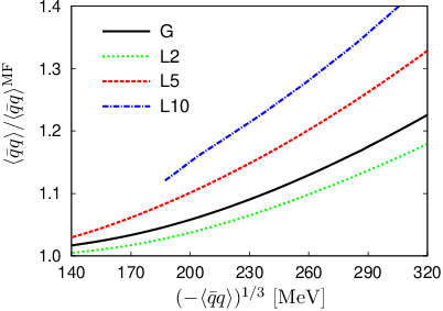
In order to study the dependence of the sign of the correction to the quark condensate on the form factor we consider the Lorentzian-type form factor with n=2,5 or 10, see also [35, 42]. We found that the sign of the correction is positive for all possible parameterizations. This is shown in Fig. 9.

A related question concerns the corrections to the quark dressing functions and , defined by
| (27) |
or, equivalently, to the wave-function renormalization function and the mass function . In mean-field approximation, we have and , see Eqs. (4) and (5). Including corrections we find that the vector dressing function becomes enhanced, corresponding to a reduction of . However, the scalar dressing function increases even stronger, so that the mass function is enhanced as well.


In Fig. 10 we present a comparison of the behavior of the mass function (upper panel) and wave-function renormalization function (lower panel) in the present approach for two parameter sets (No. 2 and No. 4) with lattice data for this quantity [18] extrapolated to the chiral limit case. One can see that the gross behavior of the momentum dependence of the quark mass function as measured in lattice QCD is reflected by the nonlocal model. More in detail, the corrected result for the weaker coupling No. 2 (thin black solid line) matches the quark mass at zero-momentum, but stays above the lattice data for dynamical quarks at finite momentum transfer. The stronger coupling set No. 4 (bold black solid line), however, overestimates the quark mass function for low momenta GeV2 by about 25% and stays below the lattice data by about the same amount in the intermediate momentum range .
As one can see in the lower panel of Fig. 10, the agreement of our model results for the wave-function renormalization function with the lattice data is rather poor. This is not unexpected because Dyson-Schwinger QCD calculations find a 30% reduction of at low momenta already in quenched approximation, i.e., without including meson effects [43], whereas the present model predicts at mean field. A nontrivial mean-field can be obtained in the nonlocal PNJL model by adopting a suitable separable form of the interaction with vector currents with derivative coupling (rank-2 interaction), see [44, 45, 16, 46] where also a comparison with lattice QCD data can be found. In the present work which uses a separable ansatz in the scalar-pseudoscalar channel (rank-one interaction), a nontrivial wave-function renormalization arises only from the corrections. Since these contributions generally do not exceed the 10% level when compared to the mean-field, we cannot expect a quantitative description of at low momenta.

In Fig. 11 we show the correction to as a function of the dimensionless coupling . Besides the total correction (black solid line), which is almost independent of the parameter choice, the contributions of the diagrams (a) and (b) of Fig. 3 are also indicated separately. As one can see, the dominant contribution comes from diagram (b), which is always positive.
Indeed, in Euclidean space the contribution of diagram (b) to the -function takes the form
| (28) |
where we have defined and
| (29) |
The latter is a straightforward extension of Eqs. (7) and (10) to (Euclidean) off-shell momenta. In particular, is strictly positive. Hence, the pion gives a positive contribution to , while the sigma contribution is negative because of the extra minus sign. Since the pions are more important, both, because of their lower mass and because of the degeneracy factor of 3, the total contribution is positive, as we have seen in Fig. 11.
Neglecting the form factors and the momentum dependencies of the quark masses and coupling constants, Eq. (28) has a natural interpretation in terms of a simple model where the quarks are coupled to pions and sigma mesons by a Yukawa interaction,
| (30) |
From this point of view, the observed enhancement of the -function through pion loops should be the expected result. This seems to be in conflict with the Dyson-Schwinger analysis of Ref. [43] where pion loops give a negative contribution to the -function in QCD. However, in that approach the pions have been introduced somewhat differently, namely through corrections to the quark-gluon vertex. It is interesting that this leads to the opposite sign. Understanding this different behavior deserves further study.
At first sight, our results also seem to contradict the analysis of Ref. [33] in a local NJL model, where again it was found that the -function decreases when pion and sigma loops are included. In contrast to our present model, the -corrections have been included selfconsistently, i.e., the calculations take into account the back-reactions of the meson loops on the mean-field selfenergy. A closer inspection [47] reveals that this is the essential difference. Whereas, in complete agreement with our expectations, the meson loops themselves give a positive contribution to the -function, their back-reaction strongly reduces the Hartree contribution, so that the total effect is a reduction of . In turn, this suggests that the enhancement of we obtain in our model could be due to the non-selfconsistent treatment of the -corrections. On the other hand, it is a well-known problem of the fully selfconsistent scheme that the internal pions are much too heavy, so that in Ref. [33] the (positive) contribution of the pion loops is underestimated. Hence, the true sign of the correction is the result of a delicate interplay between several different processes and certainly needs further investigations.
III Finite temperature
In this section we extend the model to finite temperature and then discuss the predictions for the pressure, the behavior of the quark condensate and critical temperatures.
III.1 Thermodynamic potential
The model can easily be extended to finite temperature using a -derivable ansatz (see, e.g., Ref. [48]) supplemented by the expansion. The central quantity for the analysis is the thermodynamic potential per volume
| (31) |
where and are the full propagator and the quark selfenergy, respectively, and denotes the trace over all degrees of freedom, internal ones and 4-momenta. At nonzero temperature, we also take into account the Polyakov-loop dynamics which no longer decouples from the quark sector. To that end a constant temporal background gauge field is minimally coupled to the quarks and a Polyakov loop potential is added in Eq. (31). Here denotes the Polyakov loop expectation value and its conjugate. In order to avoid confusion with the potential of the -derivable scheme (“ functional”), we denote the latter as . In the exact case, contains all two-particle irreducible diagrams. Finally, we have introduced a subtractive renormalization constant , which is chosen such that the vacuum () has vanishing pressure.
The thermodynamic equilibrium corresponds to the (global) minimum of the thermodynamic potential with respect to the full quark propagator and to the Polyakov loop, so that the following necessary conditions (gap equations) must be fulfilled
| (32) |
We work in Polyakov gauge where the background gauge field is diagonal in color space, i.e., . Following [10], we require to be real with real . As a consequence and we are left with one variable . The second and the third equation thus reduce to . Moreover, the first equation implies that . Diagrammatically this means that the quark selfenergy can be obtained from by cutting one quark line at all possible places.
Approximations can be introduced by truncating at a certain order. The mean-field results, corresponding to the leading order in , are obtained from the “glasses” diagram, displayed in Fig. 12. Solid lines represent dressed quark propagators.

In the nonlocal model the “glasses” potential takes the form
| (33) |
and the thermodynamic potential reads
where and the notation has been introduced. Note that due to the coupling to the Polyakov loop the fermionic Matsubara frequencies are partially shifted: , . Apart from this shift, the modification of the quark propagator only depends on the dynamical mass . Therefore at mean field the gap equations, Eq. (32), take the form
| (34) |
The next-to-leading order contribution to the -potential is given by the “ring sum”,
| (35) |
see Fig. 13.

Here denotes the quark-antiquark polarization functions constructed with the full quark propagators and is the mesonic degeneracy factor.
At this level, the problem arises that in a fully selfconsistent treatment the iteration of diagrams in the gap equation leads to contributions of arbitrary orders in . As a consequence, different approximation schemes can be defined. In the present paper, we use a “strict expansion”, where all contributions beyond the next-to-leading order are discarded. In the absence of the background gluon field this scheme is straightforwardly implemented by first solving the mean-field gap equation for (first equation of Eq. (34)) and then evaluating the ring sum using the mean-field propagators. Thus, one gets for the thermodynamic potential
| (36) |
with the correction
| (37) |
where the polarization functions are evaluated with mean-field propagators and summation is over bosonic Matsubara frequencies.
Including the gluon background, we suggest to treat the Polyakov-loop potential as effectively independent.55 5 In principle the is proportional to the number of gluons, [49, 50]. Its leading contribution to the thermodynamic potential is therefore of the order , while the quarks only contribute at the order and corrections are of the order for both, quarks and gluons. However, since in practice the detailed form of is not based on a expansion, but rather a phenomenological parameterization fitted to quenched lattice data, we believe that it is more appropriate to treat it as independent in the present context. A strict expansion of the thermodynamic potential then corresponds to evaluate Eq. (36) for the simultaneous solutions of the gap equations
| (38) |
Note that is determined by minimizing the total thermodynamic potential, whereas is obtained from the mean-field part only. Nevertheless, since also depends on , the value of is changed as well compared to the mean-field calculation, due to the modified value of .
We also note that the scheme outlined above slightly differs from the scheme in our previous paper [13] where both, and , have been fixed at mean-field level, before inserting them into . In the numerical calculations, however, this difference turned out to be small.
III.2 Finite temperature results
We now discuss our numerical results at finite temperature. In the quark sector we take the parameters of set No. 4, see Table 1 in Sec. II.3. For the Polyakov loop potential we adopt the logarithmic parametrization of Ref. [10], which has been fitted to the quenched lattice data of Ref. [51]. The only exception concerns the parameter , which corresponds to the transition temperature in pure gauge. While in Ref. [10] the empirical value MeV was used, it has been argued in Ref. [52] that depends on the number of active flavors and a value of MeV was suggested for . Therefore our calculations will be performed using both values of .


The model predictions for the pressure are displayed in Fig. 14. The upper panel corresponds to MeV, the lower one to MeV. Together with the full result (solid lines) we show the partial contributions to the pressure from the mean-field approximation (dash-dotted lines), , and from the corrections (dashed lines), . In agreement with earlier results in PNJL-like models we find that at low temperatures the mean-field contribution, corresponding to thermally excited quarks, is strongly suppressed by the Polyakov loop. In this regime the thermodynamics is governed by the ring sum, which is dominated by pionic degrees of freedom as the lightest particles in the mass spectrum. Therefore, it is instructive to compare our result with the predictions of chiral perturbation theory (). describes the low-energy structure of different amplitudes in terms of an expansion in powers of energies, momenta and current quark masses. The finite temperature result for the pressure is given by [53]
| (39) | |||||
where is the weak pion decay constant in the chiral limit, is the pion energy, and refers to the chiral counting scheme, where and count as quantities of order . The term proportional to just represents the free relativistic pion gas pressure, while the term is caused by interactions and leads to a small reduction of the pressure.66 6 In the chiral limit and are given by (40) The omitted terms of order are also due to interactions.
Recalling that the pion decay constant is of the order , we see that the and terms are of the order and , respectively. Comparing this with our model, where the mean-field and ring-sum contributions to the pressure are of the order and , respectively, we conclude that our model calculations should only be consistent with the lowest-order result, i.e., with the term. Nevertheless, since the -term is small (it vanishes in the chiral limit), we find excellent agreement even when this term is included, see Fig. 14. Moreover, the low-temperature behavior of our model predictions is almost insensitive to the particular functional dependence of the form factor and different parameterizations. Of course, our results start to deviate from the predictions when we approach the chiral phase transition. Near the critical temperature the meson gives an additional visible contribution whereas already for the mesonic contributions are negligible and the quark-gluon mean-field dominates the pressure.
Comparing the upper and lower panels of Fig. 14 we observe that the lowering of also leads to a lowering of the transition temperature. However, apart from this trivial effect, the results remain qualitatively unchanged.


In Fig. 15 we show the temperature dependence of the quark condensate (black solid line) and of the Polyakov loop expectation value (red dashed line) in our model beyond mean field. For comparison we also show the quark condensate in mean-field approximation (blue dash-dotted line). Again, the results for MeV and 208 MeV are displayed in the upper and in the lower panel, respectively. As already seen for the pressure, the corrections mainly affect the behavior of the chiral condensate below and around the critical region. In particular at low temperatures the reduction of the chiral condensate is almost entirely driven by the pion dynamics, which is missing in the mean-field approximation. In this context, it is again instructive to compare the model results with the prediction. The latter is given by
| (41) |
showing that the leading temperature effect is of the order . Our model results are completely consistent with this: Whereas the mean-field condensate () stays practically constant at low , we find very good agreement with the predictions (green dotted line) after including the corrections. We should note that the chiral expansion scheme is very similar but not exactly equivalent to the counting: In the leading-order correction to the chiral condensate depends on the weak pion decay constant in the chiral limit , whereas in the expansion it depends on the week pion decay constant for massive pions in mean-field approximation . Although formally of higher order in or , this could lead to quantitative differences, even at low temperatures. However, for the chosen parameters the difference between and happens to be very small.
In agreement with other works [29, 33, 54], the additional reduction of the chiral condensate by the -correction terms generally also leads to a lowering of the chiral phase-transition temperature as compared to the mean-field result. This effect is most clearly seen in the upper panel of Fig. 15, corresponding to MeV. Unfortunately, because of the perturbative nature of the strict -expansion scheme, our model cannot be applied to study the phase transition itself. In the figure, this is obvious from the existence of an unstable region (“wiggle”) in that region. The origin of this wiggle can be attributed to the momentum independent correction to the quark selfenergy (Fig. 3a). In the vicinity of the phase transition, this diagram is dramatically enhanced due to the restoration of chiral symmetry and the corresponding lowering of the intermediate -meson mass. (In fact, in the chiral limit this contribution would go to minus infinity at .) As a rough estimate we define the unstable region as the regime where the relative correction to the quark condensate is larger than . In the present example this corresponds to temperatures between and MeV. Since our results cannot be trusted in this area, we suggest to use a simple polynomial interpolation between the stable regions at lower and higher temperatures. The resulting temperature dependence is displayed in Fig. 15 by the thin black solid line.
The situation is somewhat different for MeV (lower panel). Although the corrections are again essential at low temperatures (in agreement with the results), their effect on the chiral critical temperature is almost negligible. This is due to the fact that for this lower value of the mean-field transition takes place earlier. Related to this, the mean-field chiral condensate drops more steeply77 7 For MeV, the phase transition even becomes first order. A similar observation was recently made in Ref. [16].. The “unstable region” where the relative correction to the quark condensate is larger than is quite narrow and the wiggle near the chiral phase transition, which we found for MeV, is not present for MeV.
A systematic overview about the -dependence of the pseudocritical temperatures for deconfinement (red dashed line) and chiral restoration (solid black line) is given in Fig. 16. As definitions of these temperatures we have chosen the maxima of the temperature derivatives of the corresponding order parameter, i.e., Polyakov-loop expectation value and chiral condensate, respectively. In the unstable regime (indicated by the shaded area) the latter was obtained from the polynomial interpolation. The mean-field result for the chiral-restoration temperature is also shown (blue dashed-dotted line).
In this figure, we can roughly distinguish three regimes: At large values of already the mean-field is lower than , and is even lowered further by including corrections. Then, in some intermediate regime, and agree at mean field but there is still a visible reduction of the latter by the corrections. Finally, for MeV all three lines practically coincide.88 8 According to Table 1 the corrections can even enhance the value of by 1 or 2 MeV at MeV. However, since cross-over temperatures are not defined in a unique way, and even rely on the polynomial interpolations in the present case, this should not be over-interpreted. If we had defined as the temperature where the condensate reaches half of its vacuum value, the corrections would always lead to a reduction of .

To understand this behavior we should recall that without coupling between quark and Polyakov-loop sector, corresponds to the (first-order) deconfinement-transition temperature, while the chiral cross-over in the nonlocal model takes place at a very low temperature, MeV. From this point of view it is quite remarkable that even for MeV the coupling reduces the difference between and to less than 10 MeV. Nevertheless, the synchronization obviously works better when is reduced and eventually becomes perfect for MeV. Related to this, the transitions get sharper with decreasing and the relative effect of the corrections on is reduced as well, as we have seen above.
At this point we should note that the Polyakov-loop dynamics and, hence, the deconfinement transition are quite insensitive to the corrections. This is most likely an artifact of the model where the Polyakov-loop is affected by the meson back-coupling only in a very indirect way (see the discussion after Eq. (38)). In principle, mesonic fluctuations should also directly influence the Polyakov-loop potential. However, it is not clear how to include this in PNJL-like models, where the potential is obtained from a phenomenological fit of quenched lattice data where even the effects of dynamical quarks are neglected (except for changes in ). In this context it would certainly be interesting to compare the behavior of the Polyakov loop with the so-called dressed Polyakov loop, related to the dual quark condensate [55, 56]. The latter can be calculated within PNJL-like [57] (and even NJL models [58]) and it should be possible to study corrections as well. However, this is beyond the scope of the present paper.

In Fig. 17 we present the comparison of our prediction for the temperature dependence of quark condensate and Polyakov loop with recent lattice data [19, 20]. The model calculations are performed with MeV, which leads to the more realistic transition temperatures. One should mention that the lattice calculations [19, 20] are performed for the case of two light quarks and one strange, . For the investigation of the quark condensate they use a combination of nonstrange() and strange() quark condensates, called subtracted quark condensate,
| (42) |
In the present paper we consider a model with only two light active flavors. Nevertheless, it makes sense to perform the comparison of our calculation for the temperature dependence of the quark condensate normalized to its vacuum value with the lattice calculations of the subtracted quark condensate. The reason is that the nonpertubative part of the quark condensate in Eq. (6) is finite and the strange quark contribution in Eq. (42) is suppressed in the nonlocal model by two factors: (i) the ratio of the nonpertubative part of the strange quark condensate to that of the nonstrange one is and the ratio of the nonstrange current quark mass to the strange one is about . On the other hand the main role for low temperature changes of the quark condensate is played by pions - an effect which is correctly accounted for in our model.
Indeed, we find that is rather well reproduced by our model calculations for . For the Polyakov loop, on the other hand, we find good agreement only at the onset, whereas around the deconfinement temperature, MeV, the model prediction rises much steeper than the lattice data. This seems to indicate that there is missing physics, which is not captured by just rescaling the temperature of the pure-glue potential.
IV Summary
In the present work, we have extended the nonlocal chiral quark model, coupled to the Polyakov loop, beyond the mean field approximation using a strict expansion scheme. In vacuum, it is found that corrections lead to an increase of the quark condensate, which is opposite to results obtained in the NJL model with local interactions. However, the result of the local model is strongly dependent on the mesonic cut-off and for large values of the cut-off ( GeV) the sign of the correction is positive in both models.
The parameters of the nonlocal model have been refitted in vacuum to reproduce the physical values of the pion mass and the weak pion decay constant after including the corrections. In agreement with general expectations, we find that the mean field gives the dominant contribution to the pion properties, while the maximal size of the corrections to the pion mass and weak pion decay constant amounts to 15 and 20 MeV, respectively.
At finite temperature, the corrections lead to a reduction of the chiral condensate when compared to the mean-field result. Typically, this also leads to a reduction of the chiral phase transition temperature. However, for lower values of the parameter in the Polyakov-loop potential, the mean-field transition becomes steeper and, thus, the effect of the corrections on becomes smaller. Eventually, for MeV, remains practically unaffected by the corrections. For low temperatures, MeV, our result for the quark condensate practically coincides with that of whereas the high-temperature region is well controlled by the mean-field approximation.
In the chiral limit our expansion scheme, which treats the corrections perturbatively, breaks down in the vicinity of the chiral phase transition. For the real case of nonzero current quark masses a similar situation takes place for large values of the parameters of the Polyakov loop potential (e.g., MeV in the pure gluodynamics case). Alternatively, one could include the mesonic fluctuations non-perturbatively, as done in Ref. [33] for the local NJL model. In that analysis it was found as well that mesonic fluctuations lead to a decrease of the critical temperature, but the unstable region around the phase transition is absent. On the other hand, the low-temperature behavior of is not reproduced in this scheme. It seems plausible that the inclusion of higher-order corrections could make both expansion schemes converge to one another, i.e., in the strict expansion the unstable region will be reduced (except close to a real phase transition) while in the self-consistent scheme the low-temperature behavior will get closer to the predictions.
Concerning the pressure, we confirm our previous result [13] that the pionic contribution dominates in the low temperature region. In this regime, the pressure is quite insensitive to the details of the interaction and agrees almost exactly with that of an ideal pion gas. At temperatures , on the other hand, the mesonic contributions die out at .
As a next step, we plan to study nonzero chemical potentials, which may require a nontrivial extrapolation of the Polyakov-loop potential into this regime [52]. The treatment of the entire – plane of the QCD phase diagram finally requires the inclusion of baryonic degrees of freedom as well.
Acknowledgements.
We thank C. Fischer, D. Müller, J. Wambach, and R. Williams for critical remarks and illuminating discussions. A.E.R. is grateful for the hospitality extended to him during visits at the TU Darmstadt and at the University of Wrocław. We acknowledge support by the Heisenberg-Landau programme (M.B., A.E.R., M.K.V.), by EMMI (A.E.R.), by the Russian Foundation for Basic Research under contracts No. 09-02-00749 (A.E.R.), No. 08-02-01003-a and No. 11-02-01538-a (D.B.), a grant of the Russian President (A.E.R.), and by the Polish Ministry of Science and Higher Education under the CompStar-POL grant and grant No. NN 202 231837 (D.B.), as well as by CompStar, a Research Networking Programme of the European Science Foundation. |
 |
 |
 |
 |
 | |||||
| 1a | 1b | 2a | 2b | 2c | 3a |
 |
 |
 |
 |
 | ||||
| 1c | 1d | 2d | 2e | 2f |
 |
 | |
| 3b | 3c |
Appendix A corrections to the pion propagator and the weak decay constant
The corrections to the meson propagator consist of the diagrams shown in Fig. 18. For convenience we divide them into three types. For the pion the corresponding expressions take the form
| (43) | ||||
where the factor in is the degeneracy factor.
The calculation of the weak pion decay constant is more complicated. Namely, part of the diagrams can be obtained from the pion propagator times and substitution of the outgoing pion vertex by the vertex with an external current. Furthermore, there are additional nonlocal diagrams, shown in Fig. 19.
The additional corrections of type 1 are
the corrections of type 2 take the form
and should be summed over .
The additional type-3 corrections are
where the effective vertex is
| (44) | |||||
References
- [1] Y. Nambu and G. Jona-Lasinio, Phys. Rev. 122, 345 (1961); Phys. Rev. 124, 246 (1961).
- [2] M. K. Volkov, Annals Phys. 157, 282 (1984); Sov. J. Part. Nucl. 17, 186 (1986).
- [3] S. Klimt, M. Lutz, U. Vogl and W. Weise, Nucl. Phys. A 516, 429 (1990); Nucl. Phys. A 516, 469 (1990).
- [4] S. P. Klevansky, Rev. Mod. Phys. 64, 649 (1992).
- [5] T. Hatsuda and T. Kunihiro, Phys. Rept. 247, 221 (1994).
- [6] P. N. Meisinger and M. C. Ogilvie, Phys. Lett. B 379, 163 (1996).
- [7] K. Fukushima, Phys. Lett. B 591, 277 (2004).
- [8] E. Megias, E. Ruiz Arriola and L. L. Salcedo, Phys. Rev. D 74, 065005 (2006).
- [9] C. Ratti, M. A. Thaler, and W. Weise, Phys. Rev. D 73, 014019 (2006).
- [10] S. Rößner, C. Ratti, and W. Weise, Phys. Rev. D 75, 034007 (2007).
- [11] C. Sasaki, B. Friman and K. Redlich, Phys. Rev. D 75, 074013 (2007).
- [12] H. Hansen, W. M. Alberico, A. Beraudo, A. Molinari, M. Nardi, and C. Ratti, Phys. Rev. D 75, 065004 (2007).
- [13] D. Blaschke, M. Buballa, A. E. Radzhabov and M. K. Volkov, Phys. Atom. Nucl. 71, 1981 (2008).
- [14] G. A. Contrera, D. Gomez Dumm and N. N. Scoccola, Phys. Lett. B 661, 113 (2008).
- [15] T. Hell, S. Rößner, M. Cristoforetti and W. Weise, Phys. Rev. D 81, 074034 (2010).
- [16] D. Horvatic, D. Blaschke, D. Klabucar and O. Kaczmarek, arXiv:1012.2113 [hep-ph].
- [17] K. I. Kondo, Phys. Rev. D 82, 065024 (2010).
- [18] W. Kamleh, P. O. Bowman, D. B. Leinweber, A. G. Williams, J. Zhang, Phys. Rev. D76, 094501 (2007).
- [19] A. Bazavov and P. Petreczky [HotQCD Collaboration], arXiv:1009.4914 [hep-lat].
- [20] S. Borsanyi, Z. Fodor, C. Hoelbling, S. D. Katz, S. Krieg, C. Ratti and K. K. Szabo [Wuppertal-Budapest Collaboration], JHEP 1009, 073 (2010).
- [21] J. Braun, L. M. Haas, F. Marhauser and J. M. Pawlowski, Phys. Rev. Lett. 106, 022002 (2011).
- [22] C. Amsler et al. [Particle Data Group], Phys. Lett. B 667, 1 (2008).
- [23] E. Quack and S. P. Klevansky, Phys. Rev. C 49, 3283 (1994).
- [24] D. Ebert, M. Nagy, and M. K. Volkov, Phys. Atom. Nucl. 59, 140 (1996).
- [25] E. N. Nikolov, W. Broniowski, C. V. Christov, G. Ripka, and K. Goeke, Nucl. Phys. A 608, 411 (1996).
- [26] V. Dmitrasinovic, H. J. Schulze, R. Tegen and R. H. Lemmer, Annals Phys. 238, 332 (1995).
- [27] D. Blaschke, Yu. L. Kalinovsky, G. Röpke, S. M. Schmidt and M. K. Volkov, Phys. Rev. C 53, 2394 (1996).
- [28] M. Oertel, M. Buballa and J. Wambach, Phys. Lett. B 477, 77 (2000).
- [29] M. Oertel, M. Buballa and J. Wambach, Phys. Atom. Nucl. 64, 698 (2001).
- [30] R. S. Plant and M. C. Birse, Nucl. Phys. A 703, 717 (2002).
- [31] R. G. Jafarov and V. E. Rochev, Central Eur. J. Phys. 2, 367 (2004).
- [32] K. Goeke, M. M. Musakhanov and M. Siddikov, Phys. Rev. D 76, 076007 (2007).
- [33] D. Müller, M. Buballa and J. Wambach, Phys. Rev. D 81, 094022 (2010).
- [34] G. ’t Hooft, Nucl. Phys. B 72, 461 (1974).
- [35] D. Gomez Dumm, A. G. Grunfeld, N. N. Scoccola, Phys. Rev. D74, 054026 (2006).
- [36] J. Terning, Phys. Rev. D 44, 887 (1991).
- [37] R. D. Bowler and M. C. Birse, Nucl. Phys. A 582, 655 (1995).
- [38] R. S. Plant and M. C. Birse, Nucl. Phys. A 628, 607 (1998).
- [39] A. E. Dorokhov and W. Broniowski, Eur. Phys. J. C 32, 79 (2003).
- [40] A. Scarpettini, D. Gomez Dumm and N. N. Scoccola, Phys. Rev. D 69, 114018 (2004).
- [41] M. Bhagwat, M. A. Pichowsky and P. C. Tandy, Phys. Rev. D 67, 054019 (2003).
- [42] H. Grigorian, Phys. Part. Nucl. Lett. 4, 223 (2007).
- [43] C. S. Fischer, D. Nickel, J. Wambach, Phys. Rev. D76, 094009 (2007).
- [44] S. Noguera and N. N. Scoccola, Phys. Rev. D 78, 114002 (2008).
- [45] G. A. Contrera, M. Orsaria, and N. N. Scoccola, Phys. Rev. D 82, 054026 (2010).
- [46] T. Hell, K. Kashiwa, and W. Weise, arxiv:1104.0572 [hep-ph].
- [47] D. Müller, private communication.
- [48] G. Ripka, “Quarks bound by chiral fields: The quark-structure of the vacuum and of light mesons and baryons,” Oxford, UK: Clarendon Pr. (1997).
- [49] L. McLerran, K. Redlich and C. Sasaki, Nucl. Phys. A 824, 86 (2009).
- [50] R. D. Pisarski, Phys. Rev. D 62, 111501 (2000).
- [51] O. Kaczmarek, F. Karsch, P. Petreczky and F. Zantow, Phys. Lett. B 543, 41 (2002).
- [52] B.-J. Schaefer, J. M. Pawlowski and J. Wambach, Phys. Rev. D 76, 074023 (2007).
- [53] J. Gasser and H. Leutwyler, Phys. Lett. B 184, 83 (1987).
- [54] J. Braun, Phys. Rev. D 81, 016008 (2010).
- [55] E. Bilgici, F. Bruckmann, C. Gattringer and C. Hagen, Phys. Rev. D 77, 094007 (2008).
- [56] C. S. Fischer, Phys. Rev. Lett. 103, 052003 (2009).
- [57] K. Kashiwa, H. Kouno and M. Yahiro, Phys. Rev. D 80, 117901 (2009).
- [58] T. K. Mukherjee, H. Chen and M. Huang, Phys. Rev. D 82, 034015 (2010).