The 2-3 mixing and mass split: atmospheric neutrinos and magnetized spectrometers
Abstract
We study dependence of the atmospheric and fluxes on the deviations of the 2-3 mixing from maximal, , on the -octant and on the neutrino mass splitting . Analytic expressions for the deviation effect and the octant asymmetry are derived. We present conservative estimations of sensitivities of the iron (magnetized) calorimeter detectors (ICAL) to these parameters. ICAL can establish the -deviation at higher than 3 confidence level if with the exposure of 1 Mtonyr. Sensitivity to the octant is low for zero or very small 1-3 mixing, but it can be substantially enhanced for . ICAL can measure the difference of in and channels (the CPT test) with accuracy eV2 (3) with 1 Mtonyr exposure, and the present MINOS result can be excluded at confidence level. We discuss possible ways to further improve sensitivity of the magnetized spectrometers.
pacs
14.60.Pq,14.60LmI Introduction
Determination of the 2-3 mass splitting and leptonic mixing, and in particular, the deviation of from the maximal mixing angle,
| (1) |
is of fundamental importance 11 1 is related to another deviation parameter, used in literature as .. Here we use the standard parameterization of the PMNS mixing matrix:
| (2) |
where is the matrix of rotation in the plane, and . Being maximal or close to maximal, the 2-3 mixing testifies for existence of certain underlying symmetry [1]. Comparison of the values of and as well as the mixing angles in the quarks and lepton sectors can shed some light on the origins of fermion mass and mixing in general.
The existing results on and are summarized in the Table 1. Note that the global fits of oscillation data [2] (see also [3]) show some deviation of the 2-3 mixing from maximal: (1). Although the data agree well with maximal mixing, large deviation, , is still possible.
Concerning the 2-3 mass splitting, the global fit values are in agreement with the results of SuperKamiokande (SK) [4] as well as the MINOS measurement in the channel [5].
Recently MINOS has reported the values of and in the channel [5] which differ from those in the channel (see tables 1 and 2). If confirmed, this result will testify for an effective (due to existence of some new interactions [6]) or fundamental CPT violation. The analysis of the atmospheric neutrino data does not confirm MINOS result although the sensitivity of SK to CPT violation is not high since SK sum up effects of neutrinos and antineutrinos [6]. Iron calorimeters (ICAL) [7] can perform very sensitive search for the CPT violation and check MINOS result.
New accelerator experiments T2K [8] and NOA [9] will improve precision of measurements of by factor 2, but their accuracy of measurements of will be only slightly better than that of the present global fit (see table 1).
There are two aspects of the -measurements:
- •
determination of the absolute value of the deviation , and
- •
identification of the -octant, i.e. the sign of , or in other words, resolution of the octant degeneracy.
The problem of determination of and the octant with atmospheric neutrinos has been addressed in a number of publications before [10, 11, 12, 13, 14, 15, 16]. It was realized [11, 12, 13] that at low energies oscillation effects on the electron neutrino flux are proportional to this deviation, and therefore searches for an excess (or suppression) of events in the sub-GeV range would testify for . For water Cherenkov detectors both aspects of the 2-3 mixing determinations have been explored in [12, 13]. The study was mainly concentrated on effects in the electron neutrino flux.
Magnetized calorimeters are mainly aimed at a detection of the muon neutrinos, but they can distinguish neutrinos and antineutrinos, and this composes their main advantage. These detectors provide better energy and angular resolution of the charged leptons, and consequently, neutrinos. A possibility to disentangle neutrinos and antineutrinos reinforces the following features: i) The energy and angular resolutions (reconstruction) are different for neutrinos and antineutrinos. ii) Sensitivities of the neutrino and antineutrino channels to the oscillation parameters are substantially different.
Sensitivity of a magnetized calorimeter to the 2-3 mixing and mass splitting has been explored in [14] and [15]. It has been shown that at nonzero value of the 1-3 mixing the octant discrimination is more feasible with the magnetized detector than with the water Cherenkov detector since the former can directly measure the matter effect [14]. In these studies, however, various simplifications have been made which do not allow for realistic estimations of potential of the experiments. In the analysis [17] a possibility of the octant discrimination has been evaluated for two benchmark values of and relatively high .
Here we present a comprehensive study of sensitivities of the ICAL to the parameters of 2-3 sector. We assume that by the time of operation of this detector certain information about will be obtained.
The paper is organized as follows. In sec. II we study dependence of the and fluxes on parameters of the 2-3 sector: octant and . In sec. III we describe details of our statistical analysis. We evaluate physics potential of the magnetized calorimeter to measure these parameters in sec. IV. In sec. V we consider further improvements of sensitivities of the magnetized calorimeters. Conclusions are given in sec. VI.
II Dependence of the atmospheric neutrino fluxes on 2-3 mixing
The original atmospheric neutrino flux contains both the muon, , and electron, , neutrino components, so that the muon neutrino flux at a detector equals
| (3) | |||||
Here the flavor ratio
| (4) |
is function of the neutrino energy and zenith angle .
For the standard parameterization of the mixing matrix dependence of the oscillation probabilities on the 2-3 mixing and CP-phase is explicit for an arbitrary density profile. This follows from the order of rotation in eq. (2) and the fact that the matrix of matter potentials has the form in the flavor basis, i.e. it is invariant under the 2-3 rotations. Indeed, the neutrino evolution can be considered in the propagation basis, , defined via the following relation with the flavor basis: . Consequently, , where is the basis of mass eigenstates. In the propagation basis the Hamiltonian, and therefore the amplitudes of transitions depend on , and mass squared differences:
| (5) |
and they do not depend on and . In the flavor basis, dependence of the amplitudes on these parameters appears via projections of the matrix of amplitudes (5) from the propagation basis to the flavor basis:
| (6) |
where is the matrix of amplitudes in the flavor basis.
In terms of the amplitudes using eq. (6) one can rewrite the expression for the muon neutrino flux, eq. (3), in the following form [18]:
| (7) | |||||
where
| (8) |
are the probabilities of transitions and correspondingly, and is the function which depends on the CP-violation phase . In eq. (7) is the oscillation phase due to the 2-3 mass splitting: , , etc.. Notice that , , and do not depend on .
In eq. (7) the first two terms are due to vacuum oscillations driven by the 2-3 mixing and mass splitting; the second line describes interference of the 2-3 and 1-2 modes of oscillations. The product of amplitudes in this term can be approximated as
| (9) |
The terms in the third line describe effects of oscillations due to the 1-2 and 1-3 mixing. The last term in (7) describes the CP-violation. The leading (second) term as well as the interference and CP-violating terms are symmetric with respect to change of sign of the deviation: . The octant symmetry (degeneracy) is broken by the terms in the third line of eq. (7); these terms vanish for the maximal 2-3 mixing and .
For antineutrinos one obtains the same formula as in eq. (7) with substitution and .
The octant effect can be characterized by the octant asymmetry defined as
| (10) |
For such symmetric deviations from the maximal 2-3 mixing one has
| (11) |
Then according to eq. (7) the octant asymmetry equals
| (12) |
Notice that and enter the asymmetry with opposite signs, and therefore partly cancel each other.
To get an idea about dependences of the probabilities on the neutrino parameters one can use expressions for the amplitudes in medium with constant density:
| (13) |
The probability decreases with energy, whereas increases being resonantly enhanced in the neutrino channel (for the normal mass hierarchy) at high energies. Here sensitivity of ICAL to the sign of muon charge will play important role. The two probabilities become comparable at 1 GeV for .
In the limit of zero 1-3 mixing , , and one finds from eq. (7)
| (14) |
where , which is the probability of oscillations driven by and . For the octant asymmetry we obtain
| (15) |
At low energies: and therefore the asymmetry equals .
In fig. 1 we show the oscillograms for the octant asymmetry, that is, the lines of equal asymmetry in the plane in neutrino and antineutrino channels. According to eq. (15) these oscillograms coincide with the oscillograms for up to coefficient which weakly depends on and at GeV. We use , and other parameters are set at their best-fit values. The asymmetry increases with decrease of the neutrino energy. Maximal asymmetry is achieved in the 1-2 resonance ( GeV): . For realistic threshold GeV and the averaged asymmetry is about (2 - 3)% and for GeV it is below 1%.
Notice that the octant asymmetry of flux is about 4 times larger than the flux asymmetry:
| (16) |
Here, however, the original flux is 2 times smaller. Furthermore, detection of muons provide better energy and direction resolutions.
Since and are of the same order, separation of the neutrino and antineutrino signals has no sense here.
Let us consider variations of the -flux due to deviation of the 2-3 mixing from maximal. According to (7) the relative change of the flux, which we will call the deviation effect, equals
| (17) | |||||
where in the last equality we have averaged the oscillations due to large mass splitting.
Ratio of the octant asymmetry and the 2-3 deviation effect equals
| (18) |
where and are the probabilities averaged over the experimental ranges. Although is proportional to square of the deviation parameter, for not very small () and , the integral effect of the deviation from maximal mixing is stronger than the effect of octant. The reason is that the deviation effect does not change with energy, whereas the octant asymmetry being proportional to quickly decreases with ( For zero 1-3 mixing and we have , and .


For non-zero 1-3 mixing at high energies the ratio of the flux differences is
| (19) |
and since does not decrease with energy the ratio is not small in contrast to the previous case.
In our studies of sensitivities to the parameters of 2-3 sector we obtain the oscillation probabilities solving numerically full three flavor evolution equation and using the Preliminary Reference Earth Model (PREM) [19] for the density profile of the Earth. We will use the consideration presented in this section for interpretation of the numerical results.
III The analysis for ICAL
To evaluate physics potential of the atmospheric neutrino studies with a magnetized ICAL detector we generated the atmospheric neutrino events and considered the muon energy and direction (directly measurable quantities) using event generator NUANCE-v3 [20]. The GEANT [21] simulation of ICAL detector shows that the energy and angular resolutions of muons are very high and the corresponding uncertainties are negligible compared to differences between the angles as well as energies of the neutrino and muon in the scattering (production) process.
is calculated according to the Poisson distribution. The term due to contribution of prior information on the oscillation parameters measured by other experiments is not added to here for conservative estimation; the effect of priors will be considered in sec. V. The data have been binned in cells of equal size in the ( - ) plane, where is the length of neutrino trajectory. Choice of this binning is motivated by pattern of the oscillation probability in the plane [22]. The distance between two consecutive oscillation peaks in this plane increases (decreases) as one goes to lower () values for a given (). The binning of has been optimized to get better sensitivity to the oscillation parameters. To maintain in Monte Carlo simulation study, number of events should be per cell [17]. If the number is smaller than 4 (which happens in the high energy bins), we combine results from the nearest cells.
For each set of oscillation parameters we integrate the atmospheric neutrino flux at the detector over the energy and zenith angle folding it with the cross-section, the exposure time, the target mass, the efficiency of detection and the two dimensional energy-angle correlated resolution functions to obtain data for the analysis. We use the charge current cross section of NUANCE-v3 [20] and the neutrino flux of the 3-dimensional scheme [23].
The systematic uncertainties of the atmospheric neutrino flux are crucial for determination of the oscillation parameters. We have divided them into two categories: (i) the overall flux normalization uncertainties which are independent of the neutrino energy and zenith angle, and (ii) the spectral tilt uncertainties which depend on and . The flux with uncertainties included can be written as
| (20) |
For GeV we take the energy-dependent uncertainty: and GeV, and for GeV correspondingly, and GeV. The uncertainty is in the range GeV. The overall flux uncertainty as function of the zenith angle is parameterized by . According to [23] we use which leads to 2% vertical/horizontal flux uncertainty. We take for the overall flux normalization uncertainty and for the neutrino cross-section uncertainty: .
In our analysis the numbers of events have been computed for the theoretical (fit) values and experimental (true) values of parameters in the same way by migrating the number of events from the neutrino to muon energy and zenith angle bins. The resolution functions have been taken from the previous work [24].
In studies of sensitivity to the 2-3 mixing we marginalize over , for ’s and ’s separately. Then we find the total as . We have chosen the following benchmark values of the neutrino parameters: eV2, , eV2 and . In marginalization we use, first, flat distributions of values of the parameters in the following ranges: eV2, and . The range of is changed for some particular analyses. (The non-flat distributions of parameters will be considered in sec. V.)
The parameters and produce subleading effects on the atmospheric neutrino fluxes for GeV. Moreover, effect of these parameters in marginalization is very small due to their narrow allowed regions. Therefore we have taken fixed values of and in our analysis.


IV Sensitivities of ICAL
In our computations we explored the neutrino energy range (0.141 -15) GeV, we used different energy thresholds and different exposures, , of 0.25, 1, 2, and 4 Mtonyr.
IV.1 Determination of 2-3 mixing for
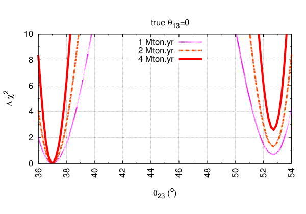
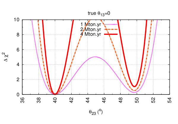
The sensitivity of ICAL experiment to is shown in fig. 2. We plot
| (21) |
as function of the fit value for fixed input values , (left) and (right) with 1, 2, and 4 Mtonyr. We have marginalized with respect to all the oscillation parameters except . The figure shows high sensitivity to the deviation : it would be possible to discriminate between a given and maximal mixing at 99% C.L., if . For instance, after 1 Mtonyr the angle can be distinguished from at level.
The figure shows also low sensitivity of the experiment to the octant. Indeed, is higher in the right minima which correspond to the wrong octant. After 1 Mtonyr exposure the difference of in the true and wrong octants is smaller than 1. The difference becomes more than 2 (90% CL) only after 4 Mtonyrs. Identification of the octant becomes even more difficult for smaller . If we find for Mtonyr. This result can be readily seen from our analytical consideration in sec. II. The probability averaged over the energy interval GeV equals , so that for : , whereas - an order of magnitude larger. As we mentioned before, this big difference of sensitivities to the deviation and octant (degeneracy) is because the octant asymmetry is collected only at very low energies where is unsuppressed, whereas whole energy range contributes to the sensitivity to the deviation .
The sensitivity to drops down substantially with decrease of . Reducing from to (compare the left and right panel of fig. 2) leads to decrease of the flux difference of eq. (17) by factor 2.5, and correspondingly, significance of discrimination from maximal mixing becomes (for Mtonyr). Sensitivity to the octant at the level appears only if Mtonyr.
In fig. 3 we show the marginalized , calculated at the maximal mixing (fit value) for different input (true) values of :
| (22) |
The picture is complementary to that in fig. 2, and there is an approximate symmetry with respect to . The reason of sharp increase of at 42 and is related to weak dependence of the oscillation probability on around and to overall flux uncertainty.
In fig. 4 we illustrate dependence of the sensitivity to the octant on . For different input (true) values of we plotted
| (23) |
According to fig. 4, it will be possible to discriminate the octant at 90% CL if or after Mtonyr. Notice that the curves are nearly symmetric with respect to .
Due to fast decrease of with increase of energy (see fig. 1) the sensitivity to the octant disappears for high values of the threshold.
IV.2 Determination of in the presence of non-zero 1-3 mixing.
Analysis of the oscillation data testifies for the non-zero 1-3 mixing, although significance of this result is not high and zero value of is not yet excluded. The global fit at 1 C.L. gives , with 3 upper bound of , and [2]. Analysis of the solar and KAMLAND data by SNO collaboration leads to at 95% CL [25]. New and forthcoming experiments Double Chooz, Daya Bay, RENO, T2K, NOA can confirm this result with higher confidence level or put new stringent upper bound [26] which would correspond approximately to a situation with zero 1-3 mixing considered in the previous section.
By the time when ICAL will collect significant statistics the angle will be known with relatively good accuracy. To clarify an impact of this information on the determination of parameters of the 2-3 sector we have performed analysis for non-zero . For illustration purpose we use as the true value and different fit intervals with flat distribution (which could reflect errors in measurements of ).
In fig. 5 we show dependence of defined in eq. (22) on the true (input) value of for the fit value and 1 Mtonyr. Different curves correspond to different marginalization intervals of . Comparing these results with the results of fig. 3 we find that inclusion of the 1-3 mixing does not change significantly the sensitivity to . The reason is that this sensitivity follows from the main mode of the oscillations; large probability for this mode extends to higher energies and 1-3 mixing produces just additional distortion of the oscillatory pattern. However, inclusion of the 1-3 mixing makes the curve less symmetric with respect to which reflects an increase of sensitivity to the octant. Also sensitivity to the deviation weakly depends on the marginalization interval for .
Fig. 6 illustrates the sensitivity of ICAL to the octant in the presence of non-zero 1-3 mixing. We show dependence of defined in eq. (23) on the true value of for the fit value . Different curves correspond to different marginalization intervals for . There are two important features of the fig. 6. First, the sensitivity to the octant is substantially better for non-zero value of than for vanishing 1-3 mixing (fig. 6) as was also shown in previous publications [13, 27, 28, 29]. This is related to the fact that the octant asymmetry of the flux is determined now by
| (24) |
and in the interval GeV; it is much larger than being enhanced in the energy range E = (3 - 10) GeV (in the resonance channel). Furthermore, at high energies and value of the coefficient in eq. (24) becomes larger. As a result, for the octant can be identified at level () with 1 Mtonyr, as compared to for .
The second feature is significant asymmetry of the curves with respect to . The asymmetry is practically absent for fixed input value of but it increases with broadening of the marginalization interval, and more importantly, with increase of the lower border of this interval. For the curves are practically not changed with change of the interval, whereas for the sensitivity substantially decreases. For instance, taking we obtain for the interval instead of for fixed value .
This asymmetry can be readily understood from the analytic consideration of sec. II. Neglecting the effect of 1-2 mixing the flux can be presented as
| (25) |
where is an even function of the deviation (symmetric with respect to change of the octant), and
| (26) |
quickly increases with , so that for one has . Therefore for the flux has much weaker dependence on than for . In the process of marginalization over we compare the true value of the flux, , with the fit value, , and is proportional to their difference:
| (27) |
If the fit value of 1-3 mixing is fixed: , the curve is approximately symmetric with respect to change . Indeed, in this case we have from eq. (27)
| (28) |
The situation is different if varies in certain interval , and we perform marginalization over in this interval. Marginalization minimizes the difference of fluxes (eq. (27)) over for a given value of . If , then . In this case the difference of fluxes is minimal if . Indeed, since decreases with , a small value of partially compensates large value of in the second term on the right hand side of eq. (27). Furthermore, the smaller the stronger compensation, and therefore the smaller can be obtained. If , then . Now to compensate the first term in eq. (27) one should take . This is, however, not possible for the considered values of . Thus, in the case of unprecise determination of sensitivity to the octant is higher for .


IV.3 Determination of the 2-3 mass split. CPT test
Important advantage of a magnetized calorimeter is that it allows one to measure the neutrino mass differences and mixing angles in the neutrino and antineutrino channel separately. A difference of results can be related to some effective or fundamental violation of the CPT symmetry.
In fig. 7 we show dependence of on the fit value of for the true value eV2 in the neutrino and antineutrino channels. We take and . According to this figure with Mtonyr the value eV2 can be discriminated from the true value at about 2 level.
The accuracy of measurement of is better in the channel. For Mtonyr the error in -channel is about two times smaller than that in channel. The difference of accuracies decreases with increase of exposure and e.g. for 1 Mtonyr it becomes about 25%. The curves are asymmetric with respect to , which is related to the dependence of oscillation probability on .
The error for could be eV2 and eV2 after 0.25 Mtonyr and 1 Mtonyr exposures correspondingly. With Mtonyr the error eV2 can be achieved at level. With Mtonyr one can obtain an accuracy eV2 ( C.L.) which is better than the present MINOS accuracy.
V Further improvements of sensitivities
There are several directions in which sensitivity of ICAL can be further improved.
V.1 Adding information about hadrons


Measurements of the hadron energy in ICAL in addition to the muon energy is expected to improve reconstruction of the neutrino energy for GeV. However, the total hadron energy in an event is carried out by multiple low energy hadrons. The average energy per hadron per event is GeV and the average number of hadrons per event is At GeV the energy resolution is very poor, roughly , and the number of hits (number of active detector layers in which signal is detected) increases only logarithmically with .
The resolution of hadron energy (for all pions and kaons) at ICAL has been obtained from GEANT4 simulation and parametrized as
| (29) |
where, and for the thickness of iron layer 5.6 cm and after averaging over all directions.
For each hadron in an event we find the reconstructed hadron energy () by a random number method using the value of from eq. 29. Then we find the final resolution as a function of ; where, is the sum of the energies of all reconstructed hadrons in an event. We use the atmospheric neutrino events without oscillations for an exposure of kTonyr generated by Nuance to reconstruct the resolution functions for each energy and zenith angle bins.
In fig. 10 we show the iso- contours with and without inclusion of information about hadrons. We find that improvement of the sensitivity to , and therefore , is marginal. Also there is a very small change in the sensitivity to : eV2.
V.2 Cross-sections and fluxes
Figs. 11 and 12 illustrate improvements of the sensitivities with reduction of different systematic uncertainties. Decrease of uncertainties of the overall flux normalization, the ratio of horizontal/vertical flux, the neutrino cross-section, and the tilt (below 1 GeV) from 10%, 10%, 2%, and 15% to 2%, 2%, 2%, and 3%, respectively, do not lead to significant improvement of the sensitivities. The reason is that the up-going neutrinos oscillate and down-going neutrinos remain practically unchanged. In analysis these down-going neutrinos allow to reduce the effect of systematic uncertainties in fluxes. Significant improvement occurs only when all systematic uncertainties are zero.


V.3 Adding priors to
In analysis in sec. 4 for simplicity we used flat distributions of uncertainties of the oscillation parameters in marginalization. The prior contribution of the parameters to . should improve the sensitivity. Proper procedure would require the use of the best-fit values and variations of parameters (especially ) which will be possible after results of forthcoming experiments will be known.


In figs. 13 and 14 we show improvements of the sensitivities to the deviation and the octant due to inclusion of the prior contribution. We have assumed the Gaussian distribution of the uncertainties around the best fit with width , and following [30, 31]. The errors in measurements of are with flat uncertainties of oscillation parameters, with prior information from present global-fit, and with prior information from possible T2K result.
The asymmetry in the sensitivity to the octant (which was due to the uncertainty of in absence of prior contribution) now disappears, and the result does not depend on marginalization range.
Of course, larger values of can substantially enhance the sensitivity to the octant since at low energies.
VI Conclusion
We have studied analytically the dependence of the deviation effect and octant asymmetry of and fluxes on the neutrino parameters and . We explored numerically a sensitivities of a magnetized calorimeter to the -deviation, to the octant and to .
We show that for the sensitivity of ICAL to the octant is low even for maximally allowed values of the deviation of the 2-3 mixing from maximal. This is related to the fact that the octant asymmetry is proportional to the “solar” probability which is large: at GeV but quickly, as , decreases with energy. The situation can be improved by lowering the threshold, increasing exposure and reducing systematic errors (especially in spectral index). We find that (octant) can be established at C.L. if , 4 Mtonyr and GeV.
ICAL has good sensitivity to the -deviation from maximal 2-3 mixing: the effect is proportional to the probability of the main channel of oscillations, , which is unsuppressed in whole considered neutrino energy range. As a result, dependence of the sensitivity on the energy threshold is weak and it does not change substantially when the effect of 1-3 mixing is included. We find that with the 1 Mtonyr exposure the accuracy of determination of the deviation will be , which is better than the present global fit result and slightly better than expected sensitivity of T2K ().
The oscillations driven by non-zero 1-3 mixing substantially improve the sensitivity to the octant. One can determine the octant for and at 90% C.L. with 1 Mtonyr exposure. We find that this sensitivity depends crucially on the uncertainty range of . For a given nonzero , the sensitivity to octant discrimination is symmetric in with respect to However, the asymmetry arises (smaller sensitivity for ) if value of can vary in large range. The symmetry is restored if prior for the 1-3 mixing is added.
The accuracy of measurements of by ICAL, eV2 (, 1 Mtonyr exposure), is two times better than the accuracy of the present global fit and it is worthier than the expected sensitivity of T2K.
ICAL can measure the difference of in and channels (the CPT test) with accuracy eV2 at 3 confidence level with 1 Mtonyr exposure and the present MINOS result can be excluded at confidence level.
We find that inclusion of information about hadrons from neutrino interactions
does not change the sensitivity to the oscillation parameters substantially.
Also improvements of the sensitivity due to better determinations
of the cross-section and neutrino flux are
rather modest. However, the sensitivity improves substantially with adding priors, especially
for the 1 - 3 mixing, and of course, with increase of the absolute value of 1-3 mixing.
Acknowledgments: The use of general cluster facility of Harish-Chandra Research Institute for a part of this work is gratefully acknowledged. A. S. wants to acknowledge Moon Moon Devi and Amol Dighe for providing the hadron resolution function.
References
- [1] R. N. Mohapatra and A. Y. Smirnov, Ann. Rev. Nucl. Part. Sci. 56, 569 (2006) [arXiv:hep-ph/0603118]; and the reference there in.
- [2] M. C. Gonzalez-Garcia, M. Maltoni and J. Salvado, JHEP 1004, 056 (2010) [arXiv:1001.4524 [hep-ph]].
- [3] G. L. Fogli, E. Lisi, A. Marrone, A. Palazzo and A. M. Rotunno, Phys. Rev. Lett. 101, 141801 (2008) [arXiv:0806.2649 [hep-ph]].
- [4] J. Hosaka et al. [Super-Kamiokande Collaboration], Phys. Rev. D 74, 032002 (2006) [arXiv:hep-ex/0604011].
- [5] P. Adamson et al. [ The MINOS Collaboration ], [arXiv:1103.0340 [hep-ex]].
- [6] J. Kopp, P. A. N. Machado and S. J. Parke, arXiv:1009.0014 [hep-ph].
- [7] V. Arumugam et al. [INO Collaboration], See, http://www.imsc.res.in/ ino/OpenReports/INOReport.pdf
- [8] I. Kato [ T2K Collaboration ], J. Phys. Conf. Ser. 136, 022018 (2008).
- [9] D. S. Ayres et al. [ NOvA Collaboration ], [hep-ex/0503053].
- [10] C. W. Kim and U. W. Lee, Phys. Lett. B 444, 204 (1998) [arXiv:hep-ph/9809491].
- [11] O. L. G. Peres and A. Y. Smirnov, Nucl. Phys. B 680, 479 (2004) [arXiv:hep-ph/0309312].
- [12] O. L. G. Peres and A. Y. Smirnov, Phys. Rev. D 79, 113002 (2009) [arXiv:0903.5323 [hep-ph]].
- [13] M. C. Gonzalez-Garcia, M. Maltoni and A. Y. Smirnov, Phys. Rev. D 70, 093005 (2004) [arXiv:hep-ph/0408170].
- [14] S. Choubey and P. Roy, Phys. Rev. D 73, 013006 (2006) [arXiv:hep-ph/0509197].
- [15] D. Indumathi, M. V. N. Murthy, G. Rajasekaran and N. Sinha, Phys. Rev. D 74, 053004 (2006) [arXiv:hep-ph/0603264].
- [16] A. Bandyopadhyay et al. [ISS Physics Working Group], Rept. Prog. Phys. 72, 106201 (2009) [arXiv:0710.4947 [hep-ph]].
- [17] A. Samanta, Phys. Rev. D 80, 113003 (2009) [arXiv:0812.4639 [hep-ph]].
- [18] E. K. Akhmedov, M. Maltoni and A. Y. Smirnov, JHEP 0806, 072 (2008) [arXiv:0804.1466 [hep-ph]].
- [19] A. M. Dziewonski and D. L. Anderson, Phys. Earth Planet. Interiors 25, 297 (1981).
- [20] D. Casper, Nucl. Phys. Proc. Suppl. 112, 161 (2002) [arXiv:hep-ph/0208030].
- [21] http://geant4.web.cern.ch/geant4/
- [22] A. Samanta, Phys. Rev. D 79, 053011 (2009) [arXiv:0812.4640 [hep-ph]].
- [23] M. Honda, T. Kajita, K. Kasahara, S. Midorikawa and T. Sanuki, Phys. Rev. D 75, 043006 (2007) [arXiv:astro-ph/0611418].
- [24] A. Samanta, Phys. Rev. D 81, 037302 (2010) [arXiv:0907.3540 [hep-ph]].
- [25] B. Aharmim et al. [SNO Collaboration], Phys. Rev. C 81, 055504 (2010) [arXiv:0910.2984 [nucl-ex]].
- [26] M. Mezzetto and T. Schwetz, J. Phys. G 37, 103001 (2010) [arXiv:1003.5800 [hep-ph]].
- [27] K. Hiraide, H. Minakata, T. Nakaya, H. Nunokawa, H. Sugiyama, W. J. C. Teves, R. Zukanovich Funchal, neutrino oscillation experiments,” Phys. Rev. D73, 093008 (2006) [hep-ph/0601258].
- [28] T. Kajita, H. Minakata, S. Nakayama, H. Nunokawa, identical detectors with different baselines,” Phys. Rev. D75, 013006 (2007) [hep-ph/0609286].
- [29] D. Meloni, O. Mena, C. Orme, S. Palomares-Ruiz, S. Pascoli, JHEP 0807, 115 (2008) [arXiv:0802.0255 [hep-ph]].
- [30] P. Huber, M. Lindner, T. Schwetz, W. Winter, JHEP 0911, 044 (2009) [arXiv:0907.1896 [hep-ph]].
- [31] P. Huber, M. Lindner, M. Rolinec, T. Schwetz and W. Winter, Phys. Rev. D 70, 073014 (2004) [arXiv:hep-ph/0403068].
- [32] P. Huber, M. Lindner, M. Rolinec, T. Schwetz and W. Winter, Nucl. Phys. Proc. Suppl. 145, 190 (2005) [arXiv:hep-ph/0412133].