Asymptotic and bifurcation analysis of wave-pinning in a reaction-diffusion model for cell polarization

Yoichiro Mori ^†^†thanks: School of Mathematics, University of Minnesota, Minneapolis MN 55455, USA. Alexandra Jilkine ^†^†thanks: Green Center for Systems Biology & Department of Pharmacology, University of Texas Southwestern Medical Center Dallas TX 75390, USA. Leah Edelstein-Keshet ^†^†thanks: Institute of Applied Mathematics and Department of Mathematics. University of British Columbia, Vancouver, B.C. Canada V6T 1Z2.

April 3, 2010

Abstract

We describe and analyze a bistable reaction-diffusion (RD) model for two interconverting chemical species that exhibits a phenomenon of wave-pinning: a wave of activation of one of the species is initiated at one end of the domain, moves into the domain, decelerates, and eventually stops inside the domain, forming a stationary front. The second (“inactive”) species is depleted in this process. This behavior arises in a model for chemical polarization of a cell by Rho GTPases in response to stimulation. The initially spatially homogeneous concentration profile (representative of a resting cell) develops into an asymmetric stationary front profile (typical of a polarized cell). Wave-pinning here is based on three properties: (1) mass conservation in a finite domain, (2) nonlinear reaction kinetics allowing for multiple stable steady states, and (3) a sufficiently large difference in diffusion of the two species. Using matched asymptotic analysis, we explain the mathematical basis of wave-pinning, and predict the speed and pinned position of the wave. An analysis of the bifurcation of the pinned front solution reveals how the wave-pinning regime depends on parameters such as rates of diffusion and total mass of the species. We describe two ways in which the pinned solution can be lost depending on the details of the reaction kinetics: a saddle-node or a pitchfork bifurcation.
Manuscript submitted to SIAM Journal of Applied Mathematics, April, 4, 2010, under review.

keywords

wave-pinning, bistable reaction-diffusion system, mass conservation, stationary front, cell polarization, Rho GTPases

1 Introduction

In a recent reaction-diffusion (RD) model for biochemical cell polarization proposed in [21] we found a wave-based phenomenon whereby a traveling wave is initiated at one end of a finite, homogeneous 1D domain, moves across the domain, but stalls before arriving at the opposite end. We refer to this behavior as wave-pinning. We observed that this phenomenon was obtained from a two-component RD system obeying a modest set of assumptions: (1) Mass is conserved and limited, i.e. there is no production or removal, only exchange between one species and the other. (2) One species is far more mobile than the other, e.g. due to binding to immobile structures, or embedding in a lipid membrane. (3) There is feedback (autocatalysis) from one form to further conversion to that form.

The biological motivation for studying our specific system comes from internal chemical reorganization that is the initial stage of polarization of a living eukaryotic cell, such as a white-blood cell, amoeba, or yeast in response to a signal. Such chemical asymmetry then organizes the downstream response of the cell (e.g. shape change, motility, division, etc). Explaining the basis for such symmetry breaking has become an important question in cell biology over the past decade, motivating such mathematical models as [20, 36, 24, 26, 5]. Our own work has focused on the role of switch-like polarity proteins called Rho GTPases, which are conserved in eukaryotic cells from amoebae to humans. Upon stimulation, levels of Rho GTPase activity rapidly redistribute across a cell. For example, some members of this family (Rac, Cdc42) become strongly activated at one end (which subsequently becomes the front of the cell [16, 23]) whereas others (such as RhoA) dominate at the opposite end (which becomes the rear [43]). Whereas in our previous work we investigated such phenomena in the context of the actin cytoskeleton and cell motion, [18, 2], here we are concerned only with the mathematical basis for the initial symmetry breaking. Originally, we explored multiple interacting Rho GTPases, to determine how interactions between several members of this family affect spatio-temporal dynamics [18, 12]. In the more recent work [21], we investigated a minimal system, consisting of a single active-inactive pair of GTPases. From a mathematical perspective, this yields an opportunity for deeper analysis. From a biological perspective, it clarifies what are minimal conditions required for symmetry breaking.

The model described here and in [21] is consequently based on the following abstraction of experimental observations about Rho proteins: (1) The protein has an active (GTP-bound) and an inactive (GDP-bound) form. (2) The active forms are exclusively found on the cell membrane; those in the fluid interior of the cell (cytosol) are inactive. (3) There is a 100-fold difference between rates of diffusion of cytosolic vs membrane bound proteins [28]. (4) Continual active-inactive exchange is essential for proper polarization. If this exchange is stopped, the cell cannot polarize [10]. (5) On the time-scale of polarization (minutes), there is little or no protein synthesis in the cell (timescale of hours), i.e. during polarization, the total amount of the given protein is roughly constant. (6) Feedback from an active form to further activation are common. A schematic diagram of our model is given in Fig. 1. Cases where this has been established experimentally include [40, 15, 27].

The RD system in this study encapsulates all the above aspects, and exhibits self-polarization as a result of the wave-like phenomenon described above. The purpose of this paper is to investigate the properties of this model. In Section 2, we formulate the model in one space dimension. We first seek to obtain a mathematically clear picture of wave-pinning. This is achieved by way of matched asymptotic calculations, presented in Section 3. Here, we shall see how the wave speed, shape and stall positions are affected by the parameters of the problem. We also briefly discuss the behavior of higher dimensional generalizations of the one-dimensional model. Next, we study the bifurcation structure of our system in 4. We delineate the parameter regime for which wave-pinning is possible, and describe the bifurcation structures that are possible for different reaction kinetics. A summary and biological implications are presented in the Discussion.

2 Model formulation

Consider a one dimensional domain $\Omega=\{x:0\leq x\leq L\}$ . Denote by $u(x,t)$ and $v(x,t)$ the concentrations of active and inactive protein respectively at position $x$ and time $t$ . This one-dimensional model would be valid for a flat cell of sufficiently small thickness so that appreciable chemical gradients do not develop in the thickness direction (Fig. 1). In this case, both membrane and cytosolic positions can be described by a single coordinate $x$ , and thus, we may treat the membrane-bound species $u$ and the cytosolic species $v$ as residing in the same domain $\Omega$ . There are biological situations that warrant models in higher spatial dimensions, and we will consider such generalizations in Section 3.4. From a mathematical point of view, however, we shall see that much of the behavior of interest is already present in the one-dimensional model.

Refer to caption — Fig. 1: Left: The cell (initially unpolarized) consists of membrane (shaded) and cytosol (white). The 1D model (1) represents the chemical distribution of two forms of a protein $(u$ , and $v)$ along the diameter of a cell, idealized as a thin flat strip of uniform thickness. (The nucleus and other nonuniform features are neglected). Right: in the RD system, $u(x,t)$ is an active protein, resident in and diffusing slowly along the membrane, $v(x,t)$ is an inactive protein diffusing in the cytosol. Interconversion is subject to positive feedback from $u$ to itself. The cell diameter is along $0\leq x\leq L$ . Cell and compartment sizes not drawn to scale.

The concentrations $u$ and $v$ satisfy the following equations


	$\displaystyle\frac{\partial u}{\partial t}$	$\displaystyle=D_{u}\frac{\partial^{2}{u}}{\partial{x}^{2}}+f(u,v),$	(1a)
	$\displaystyle\frac{\partial v}{\partial t}$	$\displaystyle=D_{v}\frac{\partial^{2}{v}}{\partial{x}^{2}}-f(u,v),$	(1b)
where $f(u,v)$ is the rate of interconversion of $v$ to $u$ , and the rates of diffusion satisfy $D_{u}\ll D_{v}$ , reflecting the fact that the membrane bound species $u$ diffuses much more slowly than the cytosolic species $v$ . The boundary conditions are
	$\frac{\partial u}{\partial x}=\frac{\partial v}{\partial x}=0,\quad x=0,L.$		(1c)

It is clear that system (1) leads to mass conservation,

\int_{\Omega}(u+v)dx=K_{\rm total},

(2)

where $K_{\rm total}$ is a time-independent constant.

The following reaction term $f(u,v)$ was proposed in [21]:

f(u,v)=\eta\left(\delta+\frac{\gamma u^{2}}{m^{2}+u^{2}}\right)v-\eta u

(3)

where $\eta,\gamma,m>0,\delta\geq 0$ are constants. The above reaction term is written as the difference between a production and a decay term. The production term can be seen as $v$ times the production rate. The production rate has a sigmoidal shape as a function of $u$ , which expresses the presence of positive feedback [22, 38]. For suitable choices of $\gamma,m$ and $\delta$ , $f(u,v)$ has the following property. The expression $f(u,v)=0$ , seen as an equation for $u$ with $v$ fixed over a suitable range, has three roots $u_{-}(v)<u_{m}(v)<u_{+}(v)$ . Moreover, $u_{\pm}(v)$ are stable fixed points of the ODE $\frac{du}{dt}=f(u,v)$ whereas $u_{m}(v)$ is an unstable fixed point. In other words, the function $f(u,v)$ is a bistable function of $u$ over a range of $v$ values. Much of the analysis to follow applies not only to the specific form of $f(u,v)$ given in (3) but to a family of reaction terms satisfying a number of properties including bistability. A precise characterization of this family will be given shortly.

We now make our equations dimensionless. We scale concentrations with $m$ and the reaction rate with $\eta$ , both of which are dictated by the form of the reaction term (see (3)). Take the domain length $L$ to be the relevant length scale. Equations (1) can be rescaled using

u=m\tilde{u},\quad v=m\tilde{v},\quad x=L\tilde{x},\quad t=\frac{L}{\sqrt{\eta D_{u}}}\tilde{t},

(4)

where $\tilde{u}$ , $\tilde{v}$ , $\tilde{x}$ , and $\tilde{t}$ are dimensionless variables. The scaling in time is chosen so that we obtain a distinguished limit appropriate for the analysis of wave-pinning (see next Section). We define:

\epsilon^{2}=\frac{D_{u}}{\eta L^{2}},\quad D=\frac{D_{v}}{\eta L^{2}}.

(5)

Given $D_{u}\ll D_{v}$ , we let $\epsilon$ be a small quantity. We let $D=\mathcal{O}(1)$ with respect to $\epsilon$ . This assumption may be written as $\sqrt{D_{v}/\eta}\approx L$ , i.e. on the timescale of the biochemical reaction, the inactive substance can diffuse across the domain. In the context of cell polarization, we have a typical cell diameter $L\approx 10\mu$ m, reaction timescale $\eta\approx 1\,$ s^-1, and diffusion coefficients $D_{u}=0.1\,\mu$ m²s^-1 and $D_{v}=10\,\mu$ m²s^-1. The dimensionless constants are then $\epsilon\approx 0.03$ and $D\approx 0.1$ .

Substituting the relationships (4) and (5) into (1) dropping the $\tilde{}$ and using the same symbol $f$ for the dimensionless reaction term, we obtain:


	$\displaystyle\epsilon\frac{\partial u}{\partial t}$	$\displaystyle=\epsilon^{2}\frac{\partial^{2}{u}}{\partial{x}^{2}}+f(u,v),$	(6a)
	$\displaystyle\epsilon\frac{\partial v}{\partial t}$	$\displaystyle=D\frac{\partial^{2}{v}}{\partial{x}^{2}}-f(u,v),$	(6b)
with boundary conditions:
	$\frac{\partial u}{\partial x}=\frac{\partial v}{\partial x}=0,\quad x=0,1.$		(6c)

Note that our domain is now $0\leq x\leq 1$ . The reaction term (3) assumes the following dimensionless form:

f(u,v)=\left(\delta+\frac{\gamma u^{2}}{1+u^{2}}\right)v-u.

(7)

The (dimensionless) total amount of protein satisfies

\int_{0}^{1}(u+v)dx=K.

(8)

where $K=K_{\rm total}/m$ . We shall henceforth work almost exclusively with the dimensionless system.

As mentioned earlier, we shall consider not only (7) but a family of reaction terms satisfying the following properties:

1.

(Bistability Condition) In some range $v_{\text{min}}\leq v\leq v_{\text{max}}$ (bistable range), the equation $f(u,v)=0$ has three roots, $u_{-}(v)<u_{m}(v)<u_{+}(v)$ . Keeping $v$ fixed within the bistable range, $u_{\pm}(v)$ are stable fixed points and $u_{m}(v)$ is an unstable fixed point of the ODE $\frac{du}{dt}=f(u,v).$ That is:

$\frac{\partial f}{\partial u}(u_{\pm}(v),v)<0,\;\frac{\partial f}{\partial u}(u_{m}(v),v)>0.$ (9)
2.

(Homogeneous Stability Condition) The homogeneous states, $(u,v)\equiv(u_{\pm}(v),v),v_{\text{min}}<v<v_{\text{max}}$ are stable states of the system (6).
3.

(Velocity Sign Condition) There is one value $v=v_{c},v_{\text{min}}<v_{c}<v_{\text{max}}$ at which the following integral $I(v)$ vanishes:

$I(v)=\int_{u_{-}(v)}^{u_{+}(v)}f(u,v)\,du.$ (10)

We assume in addition that $I>0$ for $v>v_{c}$ and $I<0$ for $v<v_{c}$ .

The first condition is the bistability condition that was mentioned earlier. The reason for the name of the third condition will become clear in the next Section. We shall see in Section 3.1 that the second condition can be reduced to the following:

\and{\left(\frac{\partial f}{\partial u}-\frac{\partial f}{\partial v}\right)}{(u,v)=(u_{\pm}(v),v)}<0.

(11)

Assuming this result, we can check that (7) satisfies the above properties for the following parameter values. For $\gamma>0$ and $\delta\geq 0$ , (7) satisfies the above conditions if and only if

\gamma>8\delta.

(12)

The corresponding bistable range is given by $v_{\text{min}}=\kappa_{+}<v<\kappa_{-}=v_{\text{max}}$ where:

\kappa_{\pm}=\frac{1}{\gamma}\left(\frac{\rho}{\omega_{\pm}}+\frac{\omega_{\pm}}{1+\omega_{\pm}^{2}}\right)^{-1},\;\omega_{\pm}=\sqrt{\frac{1-2\rho\pm\sqrt{1-8\rho}}{2(1+\rho)}},\;\rho=\frac{\delta}{\gamma}.

(13)

When $\delta=0$ , $v_{\text{min}}=2/\gamma$ and $v_{\text{max}}=\infty$ . In our computational examples, we shall make use of (7) with $\delta=0$ and $\gamma=1$ , which we record here for future reference:

f(u,v)=\frac{u^{2}v}{1+u^{2}}-u.

(14)

In this case, $u_{0}(v)$ and $u_{\pm}(v)$ can be computed explicitly:

u_{-}(v)=0,\;u_{m}(v)=\frac{v-\sqrt{v^{2}-4}}{2},\;u_{+}(v)=\frac{v+\sqrt{v^{2}-4}}{2}.

(15)

We shall often make use of the following caricature of (7):

f(u,v)=u(1-u)(u-1-v).

(16)

It is easy to check that (16) satisfies all of the above properties. For this reaction term, the bistable range is $0<v<\infty$ . This example makes certain algebraic manipulations easier than (7) or (14). In Section 4, we shall also make use of another cubic that satisfies the above conditions:

f(u,v)=-(u-1)(u-u_{m})(u+1),\;\;u_{m}=-\frac{av}{\sqrt{1+(av)^{2}}},\;a>0.

(17)

The bistable range for the model with kinetics (17) is $-\infty<v<\infty$ . At least one of the roots of this polynomial is always negative, and thus, it is no longer possible to interpret $u$ and $v$ as being concentrations of chemicals. The arguments to follow, however, never require that $u$ and $v$ be positive. Both (16) and (17) will prove useful in understanding the bifurcation structure of our system.

We now describe the behavior that we wish to explain. If we consider (6a) as a stand-alone equation for fixed $v$ , it is a scalar reaction diffusion equation of bistable type. It is well-known that such equations support propagating front solutions when posed on an infinite domain. Coupling this with (6b) on a finite domain gives rise to wave-pinning. In Fig. 2, we show simulation results for our dimensionless system (6) with the reaction terms (14) and (16). The concentrations are initialized so that $u$ is high close to $x=0$ whereas $v$ is spatially uniform. This represents a stimulus at the left end of the domain. The initial rectangular profile of $u$ develops into a steep front which propagates into the domain. The height of the front gradually changes and the front eventually comes to a halt. The left portion of the domain has a high concentration of the active species $u$ whereas the right portion of the domain has a low concentration. The spatially localized initial stimulus has been amplified to produce a stable spatial segregation of the domain into a “front” and a “back”. The one-dimensional cell has achieved polarization.

3 Asymptotic Analysis of Wave-Pinning

In this Section, we perform an asymptotic analysis of wave-pinning to obtain the speed of the wave and its stall position. We shall first deal with the 1D RD system (6) and consider its higher dimensional generalizations in Section 3.4.

3.1 Stability of the Homogeneous State

Let $(u_{s}(v),v)$ be a steady state of (6), where $u_{s}=u_{\pm}$ or $u_{m}$ . Linearize (6) about $(u_{s},v)$ :

\frac{\partial}{\partial t}\begin{pmatrix}u\\ v\end{pmatrix}=\mathcal{L}\begin{pmatrix}u\\ v\end{pmatrix}\equiv J\begin{pmatrix}u\\ v\end{pmatrix}+\frac{\partial^{2}{}}{\partial{x}^{2}}\begin{pmatrix}\epsilon^{2}u\\ Dv\end{pmatrix},\quad\quad J=\and{\begin{pmatrix}f_{u}&f_{v}\\ -f_{u}&-f_{v}\end{pmatrix}}{(u,v)=(u_{s}(v),v)}.

(18)

where $f_{u}$ and $f_{v}$ denote partial derivatives of $f$ with respect to $u$ and $v$ respectively. Here, the Jacobian of the reaction terms, $J$ , is evaluated at $(u_{s},v)$ . To study linear stability, we study the spectral properties of the operator $\mathcal{L}$ under boundary conditions (6c). We must also respect the mass constraint (8) so that the perturbations satisfy:

\int_{0}^{1}(u+v)dx=0.

(19)

Since we are on a bounded domain, we need only consider eigenvalues. We thus consider the eigenvalue problem:

\mathcal{L}\begin{pmatrix}u\\ v\end{pmatrix}=\lambda\begin{pmatrix}u\\ v\end{pmatrix}.

(20)

where $u,v$ must satisfy (6c) as well as (19). It is clear that all eigenfunctions are of the form:

\begin{pmatrix}u\\ v\end{pmatrix}=\begin{pmatrix}\alpha_{u}\\ \alpha_{v}\end{pmatrix}\cos kx

(21)

where $k=n\pi$ , $n=0,1,2,\cdots$ where $\alpha_{u}$ and $\alpha_{v}$ are constants such that $(\alpha_{u},\alpha_{v})\neq(0,0)$ . When $k\neq 0$ , $\alpha_{u}$ and $\alpha_{v}$ are arbitrary, whereas when $k=0$ , $\alpha_{u}+\alpha_{v}=0$ to satisfy (19). Is is easily seen that the eigenvalues satisfy the quadratic equation:

\lambda^{2}-\tau_{k}\lambda+\Delta_{k}=0,\;\tau_{k}=\text{tr}\mathcal{L}_{k},\;\Delta_{k}=\text{det}\mathcal{L}_{k},\;\mathcal{L}_{k}=\begin{pmatrix}-\epsilon^{2}k^{2}+f_{u}&f_{v}\\ -f_{u}&-Dk^{2}-f_{v}\end{pmatrix}

(22)

where $\text{tr}\mathcal{L}_{k}$ and $\text{det}\mathcal{L}_{k}$ denote, respectively, the trace and determinant of the $2\times 2$ matrix $\mathcal{L}_{k}$ . Let us first consider the case $k=0$ . In this case, the two solutions to the above quadratic equation are:

\lambda=0,\;\text{ or }\lambda=\tau_{0}=f_{u}-f_{v}.

(23)

If $\tau_{0}<0$ , then the second eigenvalue is negative. As the reader can easily check, as soon as we assume $\tau_{0}=f_{u}-f_{v}\neq 0$ , the eigenfunction associated with $\lambda=0$ ceases to satisfy the mass constraint. Thus, if we assume $\tau_{0}<0$ we have stability for $k=0$ . Now we turn to the case $k\neq 0$ . Both roots of (22) have negative real part if and only if $\tau_{k}<0$ and $\Delta_{k}>0$ . Since

\tau_{k}=-(D+\epsilon^{2})k^{2}+\tau_{0}<\tau_{0}

(24)

$\tau_{k}<0$ so long as $\tau_{0}<0$ .

\Delta_{k}=D\epsilon^{2}k^{4}-f_{u}(D-\epsilon^{2})k^{2}-\tau_{0}\epsilon^{2}k^{2}.

(25)

Therefore, $\Delta_{k}>0$ so long as $f_{u}<0$ and $D>\epsilon^{2}$ . The condition $D>\epsilon^{2}$ is always met since we are assuming that $\epsilon$ is small. For $u_{s}=u_{\pm}$ , $f_{u}<0$ is met by the bistability condition (9). Thus, for $f$ satisfying the bistability condition, the homogeneous stability condition of the last Section is equivalent to $\tau_{0}<0$ . This is condition (11). It is interesting that the stability condition of the ODE system with fixed $v$ ( $f_{u}<0$ ) together with the stability condition for spatially homogeneous perturbations ( $\tau_{0}<0$ ) implies stability for all wave numbers.

For $u_{s}=u_{m}$ , $f_{u}>0$ by (9). For fixed $k$ , (25) can be made negative by making $\epsilon$ sufficiently small, and thus $(u_{m}(v),v)$ is always an unstable steady state for small enough $\epsilon$ . This does not preclude the possibility that $(u_{m}(v),v)$ be a stable steady state for some finite $\epsilon$ value. Suppose $f_{u}>0$ and $\tau_{0}<0$ . Let us consider the positivity of $\Delta_{k},k\geq\pi$ :

\frac{\Delta_{k}}{k^{2}}=D\epsilon^{2}k^{2}-f_{u}(D-\epsilon^{2})-\tau_{0}\epsilon^{2}\geq D\epsilon^{2}\pi^{2}-f_{u}(D-\epsilon^{2})-\tau_{0}\epsilon^{2}.

(26)

Therefore, $(u_{m}(v),v)$ is a stable steady state of the system so long as the right-most quantity is positive. This is the case if $\epsilon$ satisfies the following bound:

\epsilon^{2}>\frac{f_{u}D}{D\pi^{2}+f_{v}}.

(27)

Since $\tau_{0}<0$ by assumption, $f_{u}<f_{v}$ and thus the right hand side of the above inequality is less than $D$ . Therefore, if $\tau_{0}<0$ , there is a range of values satisfying $\epsilon^{2}<D$ (i.e. diffusion coefficient of $u$ is smaller than that of $v$ ) for which $(u_{m}(v),v)$ is a stable steady state of (6). On the other hand, if $\tau_{0}>0$ , $(u_{m}(v),v)$ is always unstable.

For (16), it is easily seen that $(u_{m}(v),v)$ is always unstable since $f_{v}=0$ at $u=u_{m}=1$ and thus $\tau_{0}=f_{u}>0$ . For (17), $(u_{m}(v),v)$ can be stable for a range of $\epsilon$ values if $a>1$ and $v$ is in a suitable range. The stability of this middle stationary state does not play a role in the wave-pinning analysis of the next Section. However, it does play a role in determining the bifurcation structure of the system as we shall see in Section 4.3.

3.2 Asymptotic Analysis of Wave-Pinning

We now consider the dynamics of (6). There are three time scales in this model, the short, intermediate and long time scales. The intermediate time scale is of greatest interest to us, and (6) is scaled accordingly. We shall start with a brief discussion of the short time scale. Discussion of the long time scale will be deferred to the next Section.

We introduce the short time variable $t_{s}=t/\epsilon$ . Then, (6) may be rewritten as:


$\displaystyle\frac{\partial u}{\partial t_{s}}$	$\displaystyle=\epsilon^{2}\frac{\partial^{2}{u}}{\partial{x}^{2}}+f(u,v),$	(28a)
$\displaystyle\frac{\partial v}{\partial t_{s}}$	$\displaystyle=D\frac{\partial^{2}{v}}{\partial{x}^{2}}-f(u,v).$	(28b)

with no-flux boundary conditions. Assuming that $u$ admits an expansion in $\epsilon$ of the form $u=u_{0}+\epsilon u_{1}$ (and likewise for $v$ ), and substituting this into the above, we find that $u_{0}$ and $v_{0}$ satisfy the equations:


$\displaystyle\frac{\partial u_{0}}{\partial t_{s}}$	$\displaystyle=f(u_{0},v_{0}),$	(29a)
$\displaystyle\frac{\partial v_{0}}{\partial t_{s}}$	$\displaystyle=D\frac{\partial^{2}{v_{0}}}{\partial{x}^{2}}-f(u_{0},v_{0}).$	(29b)

Suppose $v_{0}$ satisfies $v_{\text{min}}<v_{0}<v_{\text{max}}$ so that $f(u_{0},v_{0})$ is bistable in $u_{0}$ . The first equation tells us that $u_{0}$ will evolve towards either $u_{+}(v_{0})$ or $u_{-}(v_{0})$ depending on whether $u_{0}(v_{0})$ is greater or less than $u_{m}(v_{0})$ . At the end of the short time scale, $v_{0}$ will have a spatial profile that is uniform whereas $u_{0}$ will assume the values of $u_{+}(v_{0})$ or $u_{-}(v_{0})$ depending on position. In other words, the domain will have segregated into regions where $u_{0}=u_{+}(v_{0})$ or $u_{-}(v_{0})$ . This profile will serve as our initial condition for the intermediate time scale. In general, this initial profile consists of multiple transition layers where $u$ switches its value from $u_{+}$ to $u_{-}$ or vice versa. If there are no transition layers, this is nothing other than the stable steady state whose stability we just studied. In this Section, we shall restrict our attention to the case when the initial profile consists only of a single transition layer. Analysis in the case of multiple transition layers is essentially the same, and will be discussed in the next Section.

We now begin the analysis in the intermediate time scale. Let $\phi(t)$ be the position of the transition layer or the front. Note that the the position of the front changes with time. We now perform a matched asymptotic calculation.

Expand $u=u_{0}+\epsilon u_{1}\cdots$ and likewise for $v$ . Substituting these expansions into (6a,b) and retaining leading order terms we have the following equations for $u_{0}$ and $v_{0}$ :


$\displaystyle 0$	$\displaystyle=f(u_{0},v_{0}),$	(30a)
$\displaystyle 0$	$\displaystyle=D\frac{\partial^{2}{v_{0}}}{\partial{x}^{2}}-f(u_{0},v_{0}).$	(30b)

Equations (30) are valid in the outer region $0\leq x<\phi(t)-\mathcal{O}(\epsilon)$ and $\phi(t)+\mathcal{O}(\epsilon)\leq x<1$ , that is, at some small distance away from the sharp transition zone at the front. Note that it is impossible to solve the above system with most initial data for $u_{0}$ and $v_{0}$ . This is the reason why we need to insert a short time scale before this intermediate time scale. During the short time scale, the arbitrary initial condition evolves into an initial profile that is admissible as an initial condition for the intermediate time scale analysis. Adding (30a,b), we find:

D\frac{\partial^{2}{v_{0}}}{\partial{x}^{2}}=0.

(31)

From (31) and boundary conditions (6c), we conclude that:

v_{0}(x,t)=\begin{cases}v_{<}(t)&0\leq x<\phi(t)-\mathcal{O}(\epsilon),\\ v_{>}(t)&\phi(t)+\mathcal{O}(\epsilon)<x\leq 1,\end{cases}

(32)

where the values of $v$ to the right and to the left of the front, $v_{>}$ and $v_{<}$ , do not depend on $x$ . From (30a), $u_{0}$ takes on one of the values $u_{+},u_{-}$ or $u_{m}$ in the outer regions. Since we are seeking a front solution, we let:

u_{0}(x,t)=\begin{cases}u_{+}(v_{<})&0\leq x<\phi(t)-\mathcal{O}(\epsilon),\\ u_{-}(v_{>})&\phi(t)+\mathcal{O}(\epsilon)\leq x<1.\end{cases}

(33)

We have assumed, without loss of generality, that $u$ transitions from $u_{+}$ to $u_{-}$ in the direction of increasing $x$ as we traverse $\phi(t)$ .

Let $w(x,t)=x-\phi(t)$ be the distance from the transition front, i.e. $w=0$ at the front. Introduce a stretched coordinate $\xi$ for the inner layer close to the evolving front:

\xi=\frac{w}{\epsilon}=\frac{x-\phi(t)}{\epsilon}.

(34)

The inner solution is denoted by $U,V$ , where

U(\xi,t)=u((x-\phi(t))/\epsilon,t),\quad V(\xi,t)=v((x-\phi(t))/\epsilon,t).

(35)

Note that (35) is not a traveling front solution in the strict sense, as the wave speed $d\phi/dt$ is not constant. As the amplitudes of $U$ and $V$ also change with time, we do not assume $u(x,t)=U(\xi)$ , but rather $u(x,t)=U(\xi,t)$ , and likewise for $V$ .

Substitute the new scaling into (6) to obtain the inner equations on $-\infty<\xi<\infty$ :


$\displaystyle\epsilon\frac{\partial U}{\partial t}-\frac{d\phi}{dt}\frac{\partial U}{\partial\xi}$	$\displaystyle=\frac{\partial^{2}{U}}{\partial{\xi}^{2}}+f(U,V),$	(36a)
$\displaystyle\epsilon\frac{\partial V}{\partial t}-\frac{d\phi}{dt}\frac{\partial V}{\partial\xi}$	$\displaystyle=\frac{D}{\epsilon^{2}}\frac{\partial^{2}{V}}{\partial{\xi}^{2}}-f(U,V).$	(36b)

Expanding $U,V$ and $\phi$ in powers of $\epsilon$ , we obtain, to leading order,


		$\displaystyle\frac{\partial^{2}{U_{0}}}{\partial{\xi}^{2}}-\frac{d\phi_{0}}{dt}\frac{\partial U_{0}}{\partial\xi}+f(U_{0},V_{0})=0,$		(37a)
		$\displaystyle\frac{\partial^{2}{V_{0}}}{\partial{\xi}^{2}}=0.$		(37b)

From (37b), it follows that

V_{0}=a_{1}(t)\xi+a_{2}(t),

(38)

where $a_{1}(t),\,a_{2}(t)$ are arbitrary functions of $t$ to be determined from matching.

We match the inner ( $V_{0}$ ) and outer ( $v_{0}$ ) solutions,

\lim_{\xi\rightarrow-\infty}V_{0}(\xi)=v_{<},\quad\lim_{\xi\rightarrow\infty}V_{0}(\xi)=v_{>}.

(39)

For these limits to exist, $V_{0}$ must be a constant in the inner layer, i.e.

v_{0}=V_{0}.

(40)

Thus, $V_{0}$ is spatially uniform throughout the domain, and is equal to the outer solution $v_{0}$ . We thus recover our observation that $v_{0}$ should be uniform by the time the dynamics in the intermediate time scale dominates. We drop the dependence of $v_{0}$ on $x$ (and $V_{0}$ on $\xi$ ).

We next consider a solution for $U_{0}$ in the inner layer. Since $V_{0}$ is spatially constant in the inner layer, (37a) is an equation in $U_{0}$ only, where $V_{0}$ is a parameter (that varies in time). We must solve the boundary value problem (37a) with the matching conditions from (33) as boundary conditions at $\pm\infty$ :

\lim_{\xi\rightarrow-\infty}U_{0}(\xi)=u_{+}(V_{0}),\quad\lim_{\xi\rightarrow\infty}U_{0}(\xi)=u_{-}(V_{0}).

(41)

Such a heteroclinic solution $U_{0}^{\phi}(\xi,V_{0})$ , unique up to translation, exists for general bistable reaction terms $f(U,V)$ [14, 22]. Multiplying (37a) by ${\partial U_{0}^{\phi}}/{\partial\xi}$ and integrating from $\xi=-\infty$ to $\xi=\infty$ , we obtain:

\frac{d\phi_{0}}{dt}\equiv c(V_{0})=\frac{\int_{u_{-}(V_{0})}^{u_{+}(V_{0})}f(s,V_{0})ds}{\int_{-\infty}^{\infty}\left({\partial U_{0}^{\phi}(\xi,V_{0})}/{\partial\xi}\right)^{2}d\xi}.

(42)

An explicit analytical expression for $c(v)$ cannot in general be obtained. An exception is when the reaction kinetics is of the form $f(u,v)=-(u-u_{+}(v))(u-u_{m}(v))(u-u_{-}(v))$ , where $u_{-}<u_{m}<u_{+}$ . In this case $c(v)$ is given by [22]:

c(v)=\frac{1}{\sqrt{2}}\left(u_{+}(v)-2u_{m}(v)+u_{-}(v)\right).

(43)

The sign of the velocity, however, is determined by the numerator of fraction in (42) and can thus be easily determined given the reaction term $f(u,v)$ . By velocity sign condition (see equation (10)) we see that $d\phi_{0}/dt$ is positive when $V_{0}>v_{c}$ and negative when $V_{0}<v_{c}$ .

By (2), we see that $u_{0}$ and $V_{0}=v_{0}$ satisfy the relation:

v_{0}+\int_{0}^{1}u_{0}dx=K.

(44)

The integral of $u_{0}$ can be approximated by contributions from the two outer regions (to left and right of the front) and a $\mathcal{O}(\epsilon)$ contribution from the inner region:

\begin{split}\int_{0}^{1}u_{0}\,dx&=\int_{0}^{\phi(t)-\mathcal{O}(\epsilon)}u_{0}\,dx+\int_{\phi(t)+\mathcal{O}(\epsilon)}^{1}u_{0}\,dx+\mathcal{O}(\epsilon)\\ &=u_{+}(v_{0})\phi_{0}(t)+u_{-}(v_{0})(1-\phi_{0}(t))+\mathcal{O}(\epsilon),\end{split}

where we have used (33) in the second equality. Discard terms of $\mathcal{O}(\epsilon)$ . The reaction-diffusion system is then reduced to the following ordinary-differential-algebraic system:

\frac{d\phi_{0}}{dt}=c(v_{0}),\quad v_{0}=K-u_{+}(v_{0})\phi_{0}-u_{-}(v_{0})(1-\phi_{0}),

(45)

where $c(v_{0})$ is given by (42). In (45), the total amount of material, $K$ , is allocated to a band of width $\phi_{0}$ at level $u_{+}$ , a band of width $1-\phi_{0}$ at level $u_{-}$ , and a homogeneous level of $v_{0}$ across the entire interval.

We now show that the front speed, $d\phi_{0}/dt$ , and the rate of change $dv_{0}/dt$ , have opposite signs. Differentiating the relation $f(u_{\pm}(v),v)=0$ with respect to $v$ and using (11) leads to

0=\and{\left(\frac{\partial f}{\partial u}\frac{du_{\pm}}{dv}+\frac{\partial f}{\partial v}\right)}{u=u_{\pm}(v)}>\left(1+\frac{du_{\pm}}{dv}\right)\and{\frac{\partial f}{\partial u}}{u=u_{\pm}(v)}.

(46)

Using (9) we conclude that:

1+\frac{du_{\pm}}{dv}>0.

(47)

Differentiating the second relation in (45) with respect to $t$ results in:

\left(1+\frac{du_{+}(v_{0})}{dv}\phi_{0}+\frac{du_{-}(v_{0})}{dv}(1-\phi_{0})\right)\frac{dv_{0}}{dt}=-(u_{+}(v_{0})-u_{-}(v_{0}))\frac{d\phi_{0}}{dt}.

(48)

Since the front position must reside within a domain of unit length, we have $0<\phi_{0}<1$ . Using this and (47), we see that the factor multiplying $dv_{0}/dt$ in (48) is positive. Since $(u_{+}-u_{-})>0$ , we conclude from (48) that $dv_{0}/dt$ and $d\phi/dt$ have opposite signs. Thus, $v_{0}$ is depleted as the wave progresses across the domain. It is interesting that this conclusion was obtained using the two conditions, bistability and homogeneous stability.

Suppose $v$ is sufficiently large initially, i.e., $v_{0}>v_{c}$ at $t=0$ . Since $d\phi_{0}/dt$ is positive for $v_{0}>v_{c}$ , $dv_{0}/dt<0$ . Thus, $v_{0}$ decreases as the front $\phi_{0}$ advances. If $v_{0}$ approaches $v_{c}$ the front will come to a halt, i.e. will become pinned. Suppose the front is pinned at $\phi_{p}$ . Then $\phi_{p}$ can be determined as follows. When the wave pins, we have

v_{c}=K-u_{+}(v_{c})\phi_{p}-u_{-}(v_{c})(1-\phi_{p}).

(49)

We can interpret (49) as a relation between $\phi_{p}$ and $K$ . We must have $0<\phi_{p}<1$ . This leads to a condition on $K$ for wave-pinning to occur:

v_{c}+u_{-}(v_{c})<K<v_{c}+u_{+}(v_{c})

(50)

that is, for wave-pinning to occur, the total concentration of chemical in the domain must fall within a range given by (50). The pinned front is stable; if the front is perturbed, it will relax back to the pinned position $\phi_{p}$ as can be seen from the velocity sign condition and the fact that $\frac{d\phi_{0}}{dt}$ and $\frac{dv_{0}}{dt}$ have opposite sign.

We now illustrate the above theory with the reaction term (16). In this case, the reaction term is a cubic polynomial in $u$ , and we may apply (43) to find an explicit expression for $c(v)$ . The leading order equations (45) become:

\frac{d\phi_{0}}{dt}=\frac{v_{0}-1}{\sqrt{2}},\quad v_{0}=K-(1+v_{0})\phi_{0}.

(51)

From (51), we find that the wave stops when $v_{0}=1\equiv v_{c}$ . Condition (50) reduces to:

1<K<3.

(52)

Solving (51) for $v_{0}$ , we obtain

\frac{d\phi_{0}}{dt}=\frac{1}{\sqrt{2}}\left(\frac{K-\phi}{1+\phi}-1\right),\quad v_{0}=\frac{K-\phi_{0}}{1+\phi_{0}}.

(53)

The position at which the wave stalls, is therefore

\phi_{p}=\frac{K-1}{2}.

(54)

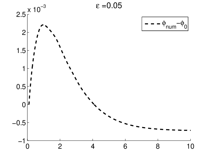
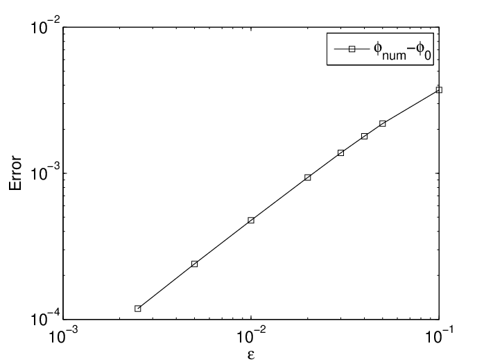
Fig. 3 shows that predictions of the ODE (53) agree with numerical solutions to the full PDE system (6) using the cubic reaction kinetics, (16). The exact front position is calculated from the numerical solution of the PDE system by tracking the position $\phi_{\text{num}}$ at which $u=u_{m}(v)$ ( $u_{m}=1$ for reaction kinetics (16)). $\phi_{\text{num}}(t_{0})$ is used as an initial condition, where $t_{0}\approx 0$ is a time at which the solution to the PDE system has relaxed to the form assumed in the asymptotic calculations. The error decreases with time as the wave becomes pinned. Based on the numerical evidence, we find that the leading order approximation is accurate to order $\epsilon$ . To get a measure of the error of the leading term approximation, we can calculate the next term in the asymptotic expression. We refer the reader to [11].

3.3 Multiple Layers and Long Time Behavior

In the previous section, we discussed the behavior of system (6) in the intermediate time scale under the assumption that the initial profile consists only of a single front. We discuss what happens when the initial profile has multiple fronts or layers. Let $\phi_{k}(t),k=1,\cdots n$ be the front positions so that $\phi_{k}(t)<\phi_{k+1}(t)$ . For notational convenience, we let $\phi_{0}(t)=0$ and $\phi_{n+1}(t)=1$ . If $u$ transitions from $u_{+}$ to $u_{-}$ as we cross a front in the positive $x$ direction, we shall call this a positive front. If the transition is from $u_{-}$ to $u_{+}$ , we call this a negative front. In the sequel, we shall assume that $\phi_{1}(t)$ is a positive front. The case in which $\phi_{1}(t)$ is a negative front can be treated in an analogous fashion. If $\phi_{1}(t)$ is a positive front, all fronts with odd $k$ are positive fronts and all fronts with even $k$ are negative fronts. Through an analysis similar to the one in the previous Section, we may conclude that the dynamics of the fronts can be tracked by the following ODE system, similarly to (45):

$\displaystyle\frac{d\phi_{k}}{dt}$	$\displaystyle=c(v)\text{ if }1\leq k\leq n\text{ is odd},$	(55)
$\displaystyle\frac{d\phi_{k}}{dt}$	$\displaystyle=-c(v)\text{ if }1\leq k\leq n\text{ is even},$	(56)
$\displaystyle K$	$\displaystyle=u_{+}(v)L_{+}+u_{-}(1-L_{+}),\quad L_{+}=\sum_{0\leq 2l\leq n}(\phi_{2l+1}-\phi_{2l}).$	(57)

For simplicity of notation, we have dropped the additional subscript showing that the above are leading order approximations. As the fronts evolve, it is possible that adjacent fronts will collide. In this case, two fronts will disappear, and the dynamics can be continued by renaming the fronts and applying the above ODE system with $n-2$ fronts instead of $n$ fronts. If front $\phi_{1}(t)$ or $\phi_{n}(t)$ hits either $x=0$ or $x=1$ respectively, one can again write down an ODE for the front positions with $n-1$ fronts valid after this incident.

As $t\rightarrow\infty$ in the above ODE system, it is possible that the final configuration will still consist of multiple fronts, despite possible annihilations of fronts that may have occurred. At this point, $v=v_{c}$ , and all fronts have velocity $0$ . As far as the intermediate time scale is concerned, these multiple front solutions are stable.

A natural question is whether these multiple front solutions will slowly evolve beyond the intermediate time scale. In this long time scale, $v$ is almost exactly equal to $v_{c}$ everywhere. We shall not include a detailed analysis of the evolution of multiple fronts in the long time scale, since the analysis and results turn out to be very similar to that of the mass-constrained Allen Cahn model, whose long time behavior has been studied extensively [41, 29, 37]. More specifically, the long time behavior of multiple front solutions of the equation:

\frac{\partial u}{\partial t}=\epsilon^{2}\frac{\partial^{2}{u}}{\partial{x}^{2}}+f(u,v_{c})-\lambda,\quad\lambda=\int_{0}^{1}f(u,v_{c})dx

(58)

with initial conditions satisfying:

v_{c}+\int_{0}^{1}udx=K

(59)

is the same to leading order to the long time behavior of the multiple front solutions of our system. In the mass-constrained Allen Cahn model, multiple front solutions are known to slowly evolve to a single front solution. Thus, multiple front solutions are metastable, and the only genuinely stable solutions are the single front solutions. The time scale of this evolution is, however, “exponentially slow” [37].

3.4 Higher Dimensions

We have thus far focused our attention on the 1D model. We may pose similar equations in higher dimensions. Given a bounded domain in $\Omega$ in $\mathbb{R}^{n}$ , we may pose the following problem:


$\displaystyle\epsilon\frac{\partial u}{\partial t}$	$\displaystyle=\epsilon^{2}\Delta u+f(u,v),$	(60a)
$\displaystyle\epsilon\frac{\partial v}{\partial t}$	$\displaystyle=D\Delta v-f(u,v),$	(60b)

with no-flux boundary conditions on the boundary $\partial\Omega$ . If $n=2$ , we may view this model as modeling a top-down view of a cell of (small) uniform thickness. Given that $u$ is a membrane bound species, it may be more appropriate in the cell biological context to study the following. Let $\Omega$ be a smooth domain in $\mathbb{R}^{3}$ whose boundary is the cell membrane $\Gamma$ . The membrane bound species $u$ resides entirely on the membrane $\Gamma$ whereas $v$ diffuses freely inside the cell. We may write down the following equations:


$\displaystyle\epsilon\frac{\partial u}{\partial t}$	$\displaystyle=\epsilon^{2}\Delta_{\Gamma}u+f(u,v)\text{ on }\Gamma,$	(61a)
$\displaystyle\epsilon\frac{\partial v}{\partial t}$	$\displaystyle=D\Delta v\text{ in }\Omega,$	(61b)
$\displaystyle-D\frac{\partial v}{\partial\mathbf{n}}$	$\displaystyle=f(u,v)\text{ on }\Gamma.$	(61c)

where $\Delta_{\Gamma}$ is the Laplace-Beltrami operator associated with the surface $\Gamma$ and $\frac{\partial v}{\partial\mathbf{n}}$ is the normal derivative of $v$ taken in the outward direction. It is easily seen that:

\frac{d}{dt}\left(\int_{\Gamma}udx+\int_{\Omega}vdx\right)=0

(62)

where $\int_{\Gamma}\cdot dx$ denotes surface integration over $\Gamma$ .

We now include a brief discussion of the behavior of these systems. We shall first focus on system (60) and comment on (61) later. In the short time scale, the domain $\Omega$ will be segregated into a portion $\Omega_{+}$ where $u\sim u_{+}$ and $\Omega_{-}$ where $u\sim u_{-}$ . The concentration $v$ is uniform throughout the domain. This serves as the initial profile for the intermediate time scale. The dynamics in the intermediate time scale may be analyzed analogously to what was done for the 1D case. Introduce a stretched coordinate near the transition layers, and perform matched asymptotics. This analysis is slightly complicated by the fact that the transition layers lie along curves if $\Omega\subset\mathbb{R}^{2}$ (or hypersurfaces if $\Omega\subset\mathbb{R}^{n}$ ) and thus, requires the introduction of curvilinear coordinates. However, to leading order in the intermediate time scale, effects due to the geometry of the transition layers turn out to be higher order. Thus, the fronts advance with the normal velocity equal to $c(v)$ where $v$ is spatially uniform and determined by mass conservation.

The dynamics in the long time scale reduces to the dynamics of the mass-constrained Allen Cahn model. The transition layers evolve by mean curvature, with the constraint that the area (or volume) of $\Omega_{+}$ must be conserved. We refer to [30, 41] for further details of the long time behavior of the mass-constrained Allen Cahn model.

The dynamics of (61) is similar. In the short time scale, $\Gamma$ segregates into domains $\Gamma_{+}$ and $\Gamma_{-}$ where the concentration of $u$ is $u_{+}$ and $u_{-}$ respectively, whereas $v$ is uniform throughout $\Omega$ . In the intermediate time scale, the transition curves that reside on $\Gamma$ advance so that the normal velocity is equal to $c(v)$ . In the long time scale, we expect that the transition layers will evolve by geodesic curvature with the constraint that the area $\Gamma_{+}$ must be conserved.

Although this long time behavior is interesting from a mathematical point of view, it is not clear whether this has any relevance in the cell biological setting since many other biochemical pathways will have come into the picture by that time.

4 Bifurcation Structure of the Wave-Pinning System

As we saw in the previous section, wave-pinning behavior occurs for small values $\epsilon$ . In this regime, the pinned single front solution (which we shall hence forth refer to as the pinned solution or pinned front) is a stable stationary solution of the system. A natural question is whether this pinned solution persists as the value of $\epsilon$ is increased. If $\epsilon^{2}=D$ (or $\epsilon=\sqrt{D}$ ) in (6) (the diffusion coefficient of the two species are the same), such stable front solutions cannot exist. We thus expect that there is some value of $\epsilon$ above which the pinned solution ceases to exist. We simulated (6) to steady state and gradually increased the value of $\epsilon$ . Fig. 4(a) and (d) show the results of sample computations when (14) and (16) are used for the reaction term. For small $\epsilon$ values, there is a gradual change in the wave shape and stall position. Beyond some $\epsilon_{c}$ , the pinned front disappears and is replaced by a stable spatially homogeneous solution. An interesting feature of this transition is that it is “abrupt”: the amplitude of the front (the difference between the maximum and minimum values of $u$ ) does not vanish gradually as $\epsilon$ approaches $\epsilon_{c}$ . In Section 4.1, we shall explore the bifurcation structure for (14) and (16). In Section 4.2, we focus on obtaining detailed information on the bifurcation structure for (16). In Section 4.3, we indicate other possible bifurcations we may expect of the pinned solution.

4.1 Bifurcation at finite $D$

For fixed $D>0$ and $K$ chosen in a suitable range, there is a stable front solution to system (6) (i.e., the pinned front) for $\epsilon$ sufficiently small. As we just saw, there is a value $\epsilon=\epsilon_{c}$ above which this pinned solution can no longer be continued. The value $\epsilon_{c}$ is thus a function of $D$ and $K$ .

To compute $\epsilon_{c}$ , we first note that stationary solutions satisfy the following system of equations:


$\displaystyle 0$	$\displaystyle=\epsilon^{2}\frac{\partial^{2}{u}}{\partial{x}^{2}}+f(u,v),$	(63a)
$\displaystyle 0$	$\displaystyle=D\frac{\partial^{2}{v}}{\partial{x}^{2}}-f(u,v),$	(63b)
$\displaystyle\frac{\partial u}{\partial x}$	$\displaystyle=\frac{\partial v}{\partial x}=0\text{ at }x=0,1,$	(63c)
$\displaystyle K$	$\displaystyle=\int_{0}^{1}(u+v)dx.$	(63d)

For fixed $D$ and $K$ , we may numerically compute $\epsilon_{c}$ by the following procedure. First, set $\epsilon=\epsilon_{0}$ sufficiently small so that the model (6) supports wave-pinning behavior. We discretize (63) and use a Newton iteration to find the stationary solution, first for $\epsilon=\epsilon_{0}$ . The solution to the above equations is far from unique, and we thus need a good initial guess to obtain the stationary solution of interest to us, the pinned solution. In order to do so, we simulate the time-dependent model (6) to steady state (i.e., run the simulation long enough) with initial conditions suitable to produce a pinned solution as $t\rightarrow\infty$ . This computed steady state serves as our initial guess to find the steady state solution at $\epsilon_{0}$ .

Once we have the pinned solution at $\epsilon_{0}$ , we may increase $\epsilon$ to $\epsilon=\epsilon_{1}>\epsilon_{0}$ and use the pinned solution at $\epsilon_{0}$ as our starting point for the Newton iteration. The stability of the newly obtained stationary solution can be monitored by computing the spectrum of the discretization of the linearized operator $\mathcal{L}$ around the computed stationary solution. This process can be repeated to find $\epsilon_{c}$ , the point above which a front solution can no longer be obtained.

Determination of $\epsilon_{c}$ using the above procedure, however, is unreliable since the Jacobian matrix for the Newton iteration becomes increasingly singular as $\epsilon$ approaches $\epsilon_{c}$ . We could not obtain values of $\epsilon_{c}$ beyond an accuracy of approximately $1.0\times 10^{-3}$ . A well-known remedy for this is to use pseudoarclength continuation [32]. Instead of using $\epsilon$ as the bifurcation parameter, one uses a pseudoarclength variable along the bifurcation curve so that we can successfully continue the solution across a fold singularity. This also gives us information on the bifurcation structure at $\epsilon=\epsilon_{c}$ .

Results from such a computation are given in Fig. 4 (panels b, c for reaction terms (14) and panels e, f for reaction terms (16)). For all values of $D$ and $K$ tested, the numerical results indicated a fold (saddle-node) bifurcation at $\epsilon_{c}$ . The pinned solution is stable until $\epsilon=\epsilon_{c}$ is reached, and this merges with a front solution which has a one-dimensional unstable direction.

The dependence of $\epsilon_{c}$ on $D$ and $K$ is plotted in Figure 5. Recall from (52) that $K_{\text{min}}=1<K<3=K_{\text{max}}$ is the wave-pinning regime for (16). For (14), the wave-pinning regime is given by (50) where $u_{\pm}$ is given in (15) and $v_{c}\approx 2.17506$ is the solution to the equation (see (10)):

I(v_{c})=\int_{u_{-}(v_{c})}^{u_{+}(v_{c})}f(u,v_{c})du=v_{c}(u_{+}(v_{c})-\arctan(u_{+}(v_{c})))-\frac{1}{2}(u_{+}(v_{c}))^{2}=0.

(64)

The wave-pinning regime is $K_{\text{min}}<K<K_{\text{max}}$ where $K_{\text{min}}=v_{c},K_{\text{max}}\approx 3.6901$ . For both (14) and (16), we sampled $K$ between $(3K_{\text{min}}+K_{\text{max}})/4<K<(K_{\text{min}}+3K_{\text{max}})/4$ .

For both reaction terms, if we fix $D$ , we see that there is a value $K=K_{m}$ at which $\epsilon_{c}$ reaches a sharp peak. The value of $K_{m}$ is located roughly at $(K_{\text{min}}+K_{\text{max}})/2$ . This may be rationalized as follows. The asymptotic calculations were based on the front being sharp and away from the boundaries. When $K=(K_{\text{min}}+K_{\text{max}})/2$ , the front is positioned approximately in the middle of the domain, and thus farthest from the boundaries. One may thus argue that $K=(K_{\text{min}}+K_{\text{max}})/2$ would tend to “maximize” the range of validity of the asymptotic calculations. The reason for the peaked appearance of the $\epsilon_{c}$ plot for fixed $D$ will be addressed toward the end of the next section.

The computed results indicate that $\epsilon_{c}$ is uniformly bounded in $D$ and $K$ . In particular, we observe that, for fixed $K$ , $\epsilon_{c}(D,K)$ tends to some value as $D$ is taken large. This serves as one motivation for studying the limit $D\rightarrow\infty$ .

4.2 Bifurcation Diagram in the limit $D\to\infty$

Here, we study the bifurcation structure of the following system:


$\displaystyle\epsilon\frac{\partial u}{\partial t}$	$\displaystyle=\epsilon^{2}\frac{\partial^{2}{u}}{\partial{x}^{2}}+f(u,v),$	(65a)
$\displaystyle v$	$\displaystyle=K-\int_{0}^{1}udx,$	(65b)

where $u$ satisfies no-flux boundary conditions at $x=0$ and $x=1$ . The above system should be seen as the limiting system of (6) when $D\rightarrow\infty$ . In this limit, $v$ is spatially uniform and hence the evolution of $v$ is determined completely by the mass constraint. By retracing the arguments of Section 3.2, the reader can easily check that the above system exhibits the same wave-pinning behavior as (6). In fact, the analysis is somewhat simpler. When $D$ is finite, we deduce from our asymptotic ansatz that $v$ is spatially uniform to leading order. In the case of (65), the spatial uniformity of $v$ is automatic. We note that system (65) is often referred to as the shadow system of (6), and that it has been shown to provide insight into the behavior of the original system [25, 4, 7].

In studying the bifurcation of system (65), we may proceed similarly to the finite $D$ case of the previous section. However, we shall take a different approach that will allow us to obtain a far more detailed picture of the bifurcation structure.

The steady state solutions to (65) satisfy:


$\displaystyle 0$	$\displaystyle=\epsilon^{2}\frac{\partial^{2}{u}}{\partial{x}^{2}}+f(u,v),$	(66a)
$\displaystyle\frac{\partial u}{\partial x}$	$\displaystyle=0\text{ at }x=0,1,$	(66b)
$\displaystyle v$	$\displaystyle=K-\int_{0}^{1}udx.$	(66c)

We shall view the first equation as an ODE for $u$ to be solved in the “time” variable $x$ . It is slightly more convenient to use $\tau=x/\epsilon$ as our “time” variable. Rewrite the first equation as a system of first order ODEs:


$\displaystyle u_{\tau}$	$\displaystyle=w,$	(67a)
$\displaystyle w_{\tau}$	$\displaystyle=-f(u,v).$	(67b)

Note that this ODE system possesses an “energy”. Multiplying both sides of (93) by $w=u_{\tau}$ and integrating, we obtain

w^{2}=F(u,v,B),\quad F(u,v,B)=-B+F_{0}(u,v),\quad F_{0}(u,v)=-\int_{0}^{u}2f(s,v)ds

(68)

where $B$ is an integration constant. Consider the $u-w$ phase plane that corresponds to system (67). The solution curves of (67) coincide with the level curves of the function $w^{2}=F_{0}(u,v)$ (see Fig. 6). Recall that the function $f(u,v)$ is bistable in $u$ for fixed $v$ satisfying $v_{\text{min}}<v<v_{\text{max}}$ (the bistability condition). We shall be interested only in analyzing cases in which $v$ falls within this bistable range. In this case, the function $y=F_{0}(u,v)$ for fixed $v$ has the form of a double well potential, whose local minima are at $u=u_{+},u_{-}$ and whose local maximum is at $u=u_{m}$ . A stationary solution of system (6) satisfying equation (66b) corresponds to a solution trajectory in the $u-w$ phase plane that starts and ends at the $u$ -axis (or $w=u_{\tau}=\epsilon u_{x}=0$ ). It is clear that there can only be such a trajectory if $B=F_{0}(u,v)$ as an equation for $u$ has four distinct solutions (see Fig. 6). Let the two middle roots be $u_{0}$ and $u_{1}$ (we assume $u_{0}<u_{1}$ ). Then, stationary single front solutions correspond to the “half loop” trajectory that connects $(u,w)=(u_{0},0)$ and $(u_{1},0)$ . We see immediately that such stationary single front solutions must be either monotone increasing or decreasing. In fact, the only stationary solutions (6) can have are multiple “half loop” trajectories that correspond to periodic multiple front solutions.

For every $(v,B)$ such that $F(u,v,B)=0$ has four solutions in $u$ , we have a corresponding half loop trajectory. We have, therefore, a two parameter family of half loop trajectories, and hence of possible stationary single front solutions. In the following, we shall simply refer to stationary single front solutions as front solutions. Let $\mathcal{D}_{vB}$ be the range of $(v,B)$ values for which $F(u,v,B)=0$ has four solutions. It is clear that (see Fig. 6):

\begin{split}\mathcal{D}_{vB}&=\{(v,B)\in\mathbb{R}^{2}|v_{\text{min}}<v<v_{\text{max}},\;B_{\text{min}}(v)<B<B_{\text{max}}(v)\}\\ B_{\text{min}}(v)&=\max F_{0}(u_{\pm}(v),v),\;B_{\text{max}}(v)=F_{0}(u_{m}(v),v)\end{split}

(69)

The expression for $B_{\text{max}}$ denotes the greater of the values $F_{0}(u_{+}(v),v)$ and $F_{0}(u_{-}(v),v)$ . We thus have a correspondence between $(v,B)$ values in $\mathcal{D}_{vB}$ and half-loop trajectories. The set $\mathcal{D}_{vB}$ exhausts all possible half-loop trajectories but one cannot say in general whether this correspondence is one-to-one. However, we do expect this to be true if $f$ is not too pathological. For reaction terms (16), (17) or (7), it is not difficult to see that this is indeed the case. We shall henceforth assume that this correspondence is one-to-one.

The task of finding front solutions has now been reduced to finding the suitable half-loop trajectories that satisfy (66b) and (66c). First, consider (66b). Half-loop solutions automatically satisfy $w=u_{\tau}=0$ and hence $u_{x}=0$ at the endpoints, but this does not necessarily mean that the endpoints correspond to $x=0$ ( $\tau=0$ ) and $x=1$ ( $\tau=1/\epsilon$ ). We must thus impose the condition that the domain length is $1$ . Suppose the front solution has value $u_{0}$ at $x=0$ and $u_{1}$ at $x=1$ , $u_{0}<u_{1}$ (we shall henceforth assume that our front solution is always monotone increasing, unless noted otherwise). The domain length condition reduces to:

1=\int_{0}^{1}dx=\int_{u_{0}}^{u_{1}}\frac{dx}{du}du=\epsilon\int_{u_{0}}^{u_{1}}\frac{du}{\sqrt{F(u,v,B)}}\equiv\epsilon I(v,B)

(70)

where we used (68). The above change of variables is valid because we know that the stationary front solution is monotone increasing. Note that $u_{0}$ and $u_{1}$ , being the middle roots of the equation $F(u,v,B)=0$ , are functions of $v$ and $B$ . Hence, the above integral is a function of $v$ and $B$ . Condition (66c) can, likewise, be written in the following form.

K=v+\epsilon\int_{u_{0}}^{u_{1}}\frac{udu}{\sqrt{F(u,v,B)}}\equiv v+\epsilon J(v,B).

(71)

We have thus reduced (66) to the two integral constraints (70) and (71). Furthermore, the integral constraints incorporate the fact that we seek single-front solutions; (66) is satisfied by any stationary solution. Given $\epsilon$ and the total mass $K$ , we may solve (70) and (71) for $v$ and $B$ , which in turn uniquely determine the half-loop trajectory, and hence, the solution $u$ . We note that a similar reduction is possible even when $D$ is finite. We describe this in Appendix 6.1. When $D$ is finite, however, it seems somewhat difficult to use this reduction to great effect.

Conditions (70) and (71) may be used in place of (66) as the basis for continuing the pinned solution. The use of conditions (70) and (71) has a computational advantage over the direct use of (66) since the former is a much smaller system to solve than the latter. We do note, however, that the numerical evaluation of the integrals $I(v,B)$ and $J(v,B)$ is not entirely trivial, especially when $B$ is close to $B_{\text{min}}$ . This is related to the fact that the half-loop trajectories come very close to heteroclinic or homoclinic orbits on the $u-w$ phase plane. The techniques used to overcome this difficulty are discussed in [11].

A more interesting use of the above conditions is the following. Since $\epsilon\neq 0$ , we may eliminate $\epsilon$ from (71) and (70). We have:

Q_{K}(v,B)\equiv(K-v)I(v,B)-J(v,B)=0.

(72)

If we can find the zero set of $Q_{K}(v,B)$ where $(v,B)\in\mathcal{D}_{vB}$ , we will have obtained all single front stationary solutions for a fixed value of $K$ (with $v$ in the bistable range) regardless of whether it arises as a continuation of the wave-pinned solution.

Any point on this zero set corresponds to a different front solution, and the value of $\epsilon$ can be recovered by using (70). Consider the map:

\mathcal{M}:(v,B)\longmapsto(M,\epsilon)=(M(v,B),(I(v,B))^{-1})

(73)

where the function $M(v,B)$ is chosen so that the map $\mathcal{M}$ defines a homeomorphism on $\mathcal{D}_{vB}$ . Note that the choice of $M$ is far from unique; we shall see that $M(v,B)=v$ works well for (16) and (17). Half-loop trajectories can then be parametrized by $(M,\epsilon)$ instead of $(v,B)$ . The zero-set of $Q_{K}(v,B)$ in $\mathcal{D}_{vB}$ can be mapped by $\mathcal{M}$ in a one-to-one fashion to yield a bifurcation curve on the $M-\epsilon$ plane.

Up to now, the treatment has been fully general. We now apply this methodology to the case when the reaction term is given by (16). We shall be interested in obtaining the bifurcation diagram when $1<K<3$ , the wave-pinning regime (see (52)). First, we note that $0<v$ is the bistable range. The domain $\mathcal{D}_{vB}$ is therefore an unbounded set, making it difficult to uniformly sample points in $\mathcal{D}_{vB}$ to determine the zero set of $Q_{K}(v,B)$ and hence the bifurcation curves. The following considerations allow us to restrict our search to a much smaller set. Given that $u_{0}$ and $u_{1}$ are the two middle roots of equation $F(u,v,B)=0$ , we have:

0=u_{-}(v)<u_{0}<u_{m}(v)=1<u_{1}<u_{+}(v)=1+v.

(74)

Therefore,

0<u_{0}<\int_{0}^{1}udx<u_{1}<1+v.

(75)

Using (63d),

v<v+\int_{0}^{1}udx=K<1+2v.

(76)

Therefore, we may restrict our search of the zero set of $Q_{K}(v,B)$ to the following range:

\frac{K-1}{2}<v<K.

(77)

We note in passing that a similar argument can be used to show that any single front stationary solution to (65) without restriction on $v$ (for $1<K<3$ ) must in fact satisfy $v>0$ and hence (77).

We thus numerically evaluate $Q_{K}(v,B)$ at sample points in the range $\mathcal{D}_{vB}^{K}=\mathcal{D}_{vB}\cap\{\frac{K-1}{2}<v<K\}$ to find the zero set of $Q_{K}(v,B)$ . More specifically, we fix $v$ and sample $B$ uniformly within the admissible range. If there are adjacent sample $B$ points for which $Q_{K}(v,B)$ changes sign, a zero is obtained between these values by bisection. This procedure is repeated for $v$ values uniformly sampled in (77). Where the zero set has a complicated structure, sampling is refined to clarify this structure. Once the zero-set is obtained, we use the map $\mathcal{M}$ with $M(v,B)=v$ (see (73)) to obtain a bifurcation curve in the $v-\epsilon$ plane. Computational evidence indicates that $\epsilon=(I(v,B))^{-1}$ is an increasing function of $B$ for fixed $v$ , and thus $\mathcal{M}:(v,B)\longmapsto(v,\epsilon)$ is a homeomorphism on $\mathcal{D}_{vB}$ .

We can explicitly obtain the region $\mathcal{D}_{v\epsilon}=\mathcal{M}(\mathcal{D}_{vB})$ by studying the integral $I(v,B)$ . Assuming that $I(v,B)>0$ is a decreasing function of $B$ for fixed $v$ , we have only to know the limiting values of $I(v,B)$ as $B\rightarrow B_{\text{min}}(v)$ and $B_{\text{max}}(v)$ (see (69)). As $B\rightarrow B_{\text{min}}$ for fixed $v$ , the half loop trajectories approach (half of) a homoclinic orbit or a heteroclinic orbit in the $u-w$ plane (see Fig. 6). In either case, the total “time” it takes for the orbit to complete the half loop increases as $B\rightarrow B_{\text{min}}$ . Thus, $I\rightarrow\infty$ as $B\rightarrow B_{\text{min}}$ . On the other hand, when $B\rightarrow B_{\text{max}}$ , the half-loop trajectory approaches the neutral center $(u,w)=(u_{m},0)=(1,0)$ in the $u-w$ phase plane. We may easily compute:

\lim_{B\nearrow B_{\text{max}}}I(v,B)=\frac{\pi}{\sqrt{v}}.

(78)

Therefore:

\mathcal{D}_{v\epsilon}=\{(v,\epsilon)\in\mathbb{R}^{2}|0<v,0<\epsilon<\sqrt{v}/\pi\}.

(79)

As one approaches the parabolic edge of $\mathcal{D}_{v\epsilon}$ , the amplitude( $=u_{1}-u_{0}$ ) of the front solution tends to $0$ and approaches the spatially homogeneous steady state $(u,v)=(1,v)$ . In fact, the parabolic edge is the only place where the amplitude tends to $0$ in $\mathcal{D}_{v\epsilon}$ . Combining this with (79) with (77), we obtain an upper bound $\epsilon<\sqrt{K}/\pi$ for the existence of single front solutions. As we shall see, this bound is not sharp.

To study the stability of the stationary solutions corresponding to points on the zero set, we must compute $u$ explicitly. Once we know $v$ and $B$ , we can find $u_{0}$ and $u_{1}$ . We can then numerically solve the initial value problem (67) with the initial values $u(0)=u_{0}$ and $w(0)=0$ . Up to numerical error, the computed solution should, by design, satisfy $u(\tau=1/\epsilon)=u(x=1)=u_{1}$ and $w(1/\epsilon)=u_{\tau}(\tau=1/\epsilon)=\epsilon u_{x}(x=1)=0$ . We can then linearize about $u$ the operator on the right hand side of (65). By examining the spectrum of (the discretization of) this linearized operator, we can determine linear stability of the steady state $u$ .

The resulting bifurcation curves on the $v-\epsilon$ plane are given in Fig. 7. When $K\neq 2$ , we found that there was at most one front solution that corresponds to each value of $v$ (or equivalently, $Q_{K}(v,B)=0$ had at most one solution in $B$ for fixed $v$ ).

We first consider the case $K<2$ (left panel). For small values of $\epsilon$ , there are three front solutions. In order of increasing $v$ , we denote these solutions $(u,v)=(u^{-}_{\epsilon}(x),v^{-}_{\epsilon}),(u^{\text{wp}}_{\epsilon}(x),v^{\text{wp}}_{\epsilon})$ and $(u^{+}_{\epsilon}(x),v^{+}_{\epsilon})$ , which we call the minus, middle and plus branches respectively.

The pinned solution corresponds to the middle branch $(u^{\text{wp}}_{\epsilon}(x),v^{\text{wp}}_{\epsilon})$ . The value $v^{\text{wp}}_{\epsilon}$ approaches $1$ as $\epsilon\rightarrow 0$ . We know from our asymptotic calculations that the integral $\int_{u_{0}}^{u_{1}}f(u,v)du$ vanishes to leading order when the wave stalls. This happens when the three roots $u_{\pm}(v)$ and $u_{m}(v)$ are equally spaced, which corresponds to $v=1$ . In the $u-w$ phase plane, $u^{\text{wp}}_{\epsilon}$ approaches a heteroclinic orbit that connects the two saddle points $(u,w)=(0,0)$ and $(u,w)=(2,0)$ .

The other two front solutions are unstable and have a one-dimensional unstable direction. The values $v^{-}_{\epsilon}$ and $v^{+}_{\epsilon}$ approach $v=(K-1)/2$ and $v=K$ respectively as $\epsilon\rightarrow 0$ . Let us consider the plus branch. As $\epsilon\rightarrow 0$ , $B$ approaches $B_{\text{min}}$ . In the $u-w$ phase plane, $u^{+}_{\epsilon}$ approaches (half of) a homoclinic orbit that originates and ends at the saddle point $(u,w)=(0,0)$ . As $u^{+}_{\epsilon}$ approaches this homoclinic orbit, the amount of “time” that the solution stays close to the saddle point increases, so that $u^{+}_{\epsilon}$ is very close to $0$ for much of the interval $0<x<1$ . Near $x=1$ , there is a sharp transition zone in which $u^{+}_{\epsilon}$ makes a steep increase to $u_{1}$ . This transition zone becomes increasingly narrow as $\epsilon\rightarrow 0$ . We may say that the solution $(u^{+}_{\epsilon}(x),v^{+}_{\epsilon})$ approaches the stable homogeneous steady state $(u,v)=(0,K)$ as $\epsilon\rightarrow 0$ . The convergence of $u^{+}_{\epsilon}(x)$ to $0$ is only uniform outside of an arbitrarily small neighborhood of $x=1$ . We can use the above phase plane information together with (71) to find the following approximate expression for $v^{+}_{\epsilon}$ when $\epsilon$ is small:

\begin{split}v^{+}_{\epsilon}&=K-\alpha_{+}\epsilon+o(\epsilon),\\ \alpha_{+}&=\lim_{B\searrow 0}J(K,B)=2\sqrt{2}\ln\left(\frac{\sqrt{\beta_{+}}+\sqrt{\beta_{-}}}{\sqrt{\beta_{+}-\beta_{-}}}\right),\\ \beta_{\pm}&=\frac{1}{3}\left(2(2+K)\pm\sqrt{2(2K+1)(K-1)}\right).\end{split}

(80)

where $o(\epsilon)$ is the usual Landau symbol denoting an expression that tends to $0$ as $\epsilon\rightarrow 0$ . Note that the expression inside the square root in $\beta_{\pm}$ is positive since $K>1$ . The validity of this expression is supported by computational results.

The situation for the minus branch is similar. As $\epsilon\rightarrow 0$ , $v^{-}_{\epsilon}\rightarrow(K-1)/2$ . In the $u-w$ phase plane, $u^{-}_{\epsilon}$ approaches half of the homoclinic orbit originating from the saddle point $(u,w)=((K+1)/2,0)$ . The value of $u^{-}_{\epsilon}$ is close to $(K+1)/2$ for most of $0<x<1$ except for a small neighborhood around $x=0$ . The function $u^{-}_{\epsilon}$ converges uniformly to $(K+1)/2$ on any set outside an arbitrarily small neighborhood around $x=0$ . Similarly to (80), we can obtain the following expression for $v^{-}_{\epsilon}$ :

\begin{split}v^{-}_{\epsilon}&=\frac{K-1}{2}+\alpha_{-}\epsilon+o(\epsilon),\\ \alpha_{-}&=\sqrt{2}\ln\left(\frac{\sqrt{\gamma_{+}}+\sqrt{\gamma_{-}}}{\sqrt{\gamma_{+}-\gamma_{-}}}\right),\;\gamma_{\pm}=\frac{1}{3}\left(2K\pm\sqrt{\frac{1}{2}(3+K)(3-K)}\right).\end{split}

(81)

Note that the expression inside the square root in $\gamma_{\pm}$ is positive since $K<3$ . The validity of the above expression is supported by numerical results.

As $\epsilon$ is increased, there is a value $\epsilon=\epsilon^{+}_{\text{sn}}$ at which the middle and plus branches meet in a saddle-node bifurcation. At this point, the disappearance of the stable front solution (the middle branch) is “abrupt” in the sense that the amplitude of $u$ is non-zero as the bifurcation is approached. This can be seen from the fact that this saddle-node bifurcation occurs in the interior of $\mathcal{D}_{v\epsilon}$ (see discussion after (79)).

The minus branch can be continued until it merges with a spatially homogeneous unstable steady state. This happens at the parabolic edge of $\mathcal{D}_{v\epsilon}$ (see (79)). Here, there is a pitchfork bifurcation at which the homogeneous steady state gives rise to two unstable front solutions, one that is monotone increasing and the other monotone decreasing. Note that, in Fig. 7, only the bifurcation diagram of the monotone increasing front solution is plotted. There is an identical bifurcation diagram for the monotone decreasing front, and these two solutions meet with a spatially homogeneous steady state at a pitchfork bifurcation. This homogeneous steady state corresponds to $(u,v)=(1,K-1)$ . Using (79), the corresponding $\epsilon$ value $\epsilon_{\text{pf}}$ is equal to:

\epsilon_{\text{pf}}=\frac{\sqrt{v}}{\pi}=\frac{\sqrt{K-1}}{\pi}.

(82)

Linearize the operator on the right hand side of (65) around this homogeneous steady state, and call this operator $\mathcal{L}$ . We can also obtain the above value by considering the spectrum of $\mathcal{L}$ . At $\epsilon=\epsilon_{\text{pf}}$ , one of the eigenvalues of $\mathcal{L}$ corresponding to the wave number $k=\pi$ becomes positive (see Section 3.1, in particular, equation (27) in the $D\rightarrow\infty$ limit). For $1<K<3$ , expression (82) gave the least upper bound of the range of $\epsilon$ for which (not necessarily stable) single front solutions exist.

We now turn to the case $K=2$ . Let us first take a look at (72). If $v=1$ , we have:

Q_{2}(1,B)=\int_{u_{0}}^{u_{1}}\frac{1-u}{\sqrt{F(u,1,B)}}du=0.

(83)

The function $F(u,1,B)$ is symmetric about $u=1$ and thus the same is true for $u_{0}$ and $u_{1}$ (i.e. $(u_{0}+u_{1})/2=1$ ). The above integral is therefore equal to $0$ whenever it is well-defined. Therefore, all points such that $v=1$ in $\mathcal{D}_{v\epsilon}$ (i.e., $(v,\epsilon)=(1,\epsilon),0<\epsilon<1/\pi$ ) are part of the bifurcation curve for $K=2$ . For $\epsilon$ small, this $v=1$ branch of solutions corresponds to the pinned front, which is thus stable for small $\epsilon$ . We shall denote this branch by $(u^{\text{wp}}_{\epsilon},v^{\text{wp}}_{\epsilon})$ and call this the middle branch. As $\epsilon\nearrow 1/\pi$ , we expect the middle branch to merge with an unstable homogeneous steady state at a pitchfork bifurcation, just like $u^{-}_{\epsilon}$ for $K<2$ . An unstable solution cannot give rise to two stable solutions in a pitchfork bifurcation. We must conclude that the middle branch is unstable when $\epsilon$ is close to $1/\pi$ . This suggests that there must be an intermediate $\epsilon$ value between $0$ and $1/\pi$ at which the middle branch loses stability. This is indeed the case.

Just as in the $K<2$ case, there are three single front solutions in the $K=2$ case for small $\epsilon$ . We shall refer to them in the same way as in the $K<2$ case. As we saw, $v^{\text{wp}}_{\epsilon}$ is always equal to $1$ . As $\epsilon$ is increased, the minus and middle branches meet in a transcritical bifurcation at $\epsilon=\epsilon_{\text{tc}}\approx 0.2353$ . Above $\epsilon_{\text{tc}}$ , the minus branch becomes stable and the middle branch loses stability. At $\epsilon=\epsilon^{+}_{\text{sn}}\approx 0.2419$ , the minus and plus branches meet in a saddle-node bifurcation.

The $K>2$ case is similar to the $K<2$ case except for some fine details. When $\epsilon$ is small, we have three front solutions which we name in the same fashion as in the $K\leq 2$ cases. The middle branch merges with the minus branch at $\epsilon=\epsilon^{-}_{\text{sn}}$ in a saddle-node bifurcation. The branch plus branch merges with the spatially homogeneous solution at $\epsilon_{\text{pf}}=\sqrt{K-1}/\pi$ (see (82)) in a pitchfork bifurcation.

An interesting detail in the $K>2$ case is that there is a small window $2<K<K_{p}\approx 2.00672$ for which the plus branch has a stable portion (see Fig. 8). The existence of such a portion is implied by the structure of the bifurcation diagram at $K=2$ . The saddle-node bifurcation at $\epsilon^{+}_{\text{sn}}$ should persist beyond $K=2$ since saddle-node bifurcations are robust under perturbations. On the other hand, when a transcritical bifurcation is perturbed, it will generally give rise to zero or two saddle node bifurcations (see [17] for example). When $K=2$ is perturbed to $K<2$ , the transcritical bifurcation does not give rise to any saddle node bifurcations. If perturbed to $K>2$ , it gives rise to two saddle node bifurcations, one of which occurs at $\epsilon=\epsilon^{-}_{\text{sn}}$ . We shall name the other $\epsilon$ value $\epsilon=\epsilon^{0}_{\text{sn}}$ . Both bifurcation points corresponding to $\epsilon=\epsilon^{0}_{\text{sn}}$ and $\epsilon^{+}_{\text{sn}}$ lie on the $(u^{+}_{\epsilon},v^{+}_{\epsilon})$ branch.

For $2<K<K_{p}$ , there are three single front solutions over the range $\epsilon^{0}_{\text{sn}}<\epsilon<\epsilon^{+}_{\text{sn}}$ , which we refer to as the $(+,1),(+,2)$ and $(+,3)$ branches respectively in order of increasing $v$ . The $(+,1)$ and $(+,2)$ branches meet in a saddle-node bifurcation at $\epsilon^{0}_{\text{sn}}$ and $(+,2)$ and $(+,3)$ branches meet at $\epsilon^{+}_{\text{sn}}$ . The $(+,1)$ and $(+,3)$ branches are unstable whereas $(+,2)$ branch is stable. For $2<K<K_{p}$ , therefore, there is a small window of $\epsilon$ values for which there is a stable front solution that cannot be reached by continuing the pinned front solution. For $K\geq K_{p}$ , the plus branch does not have a stable portion. At $K=K_{p}$ , the saddle-node bifurcation points merge and disappear.

In Fig. 9, we show the $(K,\epsilon)$ parameter region in which there is a stable single front solution. This should be seen as a refinement of the $\epsilon_{c}$ plot in Fig. 5 that we obtained for finite $D$ . The region is peaked at approximately $K=2$ , but with some fine structure coming from the small window of front solutions that exist for $2<K<K_{p}$ . The peaked geometry of this region comes from the fact that the saddle-node bifurcations at which the pinned solution loses stability are different for $K>2$ and $K<2$ . At $K=2$ , we have a transcritical bifurcation that separates these two regimes.

It is not clear how much of the insights we obtained for $D\rightarrow\infty$ can be carried over to the finite $D$ case or to the reaction term (14). It seems plausible, however, that much of what we learned does indeed carry over. For example, we expect that there is a $K$ value (that depends on $D$ ) at which the pinned solution undergoes a transcritical bifurcation (rather than a saddle-node bifurcation) as $\epsilon$ is increased. The peaked appearance of the $\epsilon_{c}$ plot of Fig. 5 serves as circumstantial evidence for this claim.

4.3 Other Possible Bifurcation Structures

We now have a clear picture of the bifurcation structure for reaction term (16), especially when $D\rightarrow\infty$ . Given the broad similarity of the $\epsilon_{c}$ plots for (14) and (16) (see Figure 5), it is natural to expect (14) to also have a bifurcation structure with features similar to (16). This raises the question of how general our findings are. For other reaction terms that support wave-pinning, there is no reason to expect the full bifurcation structure to be similar. In particular, we can raise the following question. Except at $K=2$ , the pinned front was seen to undergo a saddle-node bifurcation in the case of (16), $D\rightarrow\infty$ . This bifurcation was “abrupt” in the sense that the front amplitude tends to a non-zero value as the bifurcation point is approached. Is the saddle-node bifurcation the only generic way in which the pinned front is lost? In particular, is it generically the case that the bifurcation is “abrupt”? The answer to both questions turn out to be negative. We shall demonstrate this with a description of the bifurcation structure for the reaction term (17). We shall see that the pinned front can arise generically via a pitchfork bifurcation from a spatially homogeneous state. The exposition will be kept brief since much of the analysis proceeds along lines similar to that of the previous section. We shall only discuss the $D\rightarrow\infty$ case. The case of $D$ finite is expected to be similar. We note in particular that computational examples can be produced in which such bifurcations occur for finite $D$ .

As we saw in Section 3.1, an interesting feature of the reaction term (17) is that the middle homogeneous steady state $(u_{m},v)$ can be stable. A similar conclusion is true in the $D\rightarrow\infty$ case. This happens when $a>1$ in (17). We shall concentrate on this case. When $a<1$ , the full bifurcation diagram turns out to be quite similar to that of (16) (the generic bifurcation is the saddle-node). We shall not discuss this case here.

As can be easily checked, $-\infty<v<\infty$ is the bistable range, and $-1<K<1$ is the range for which wave-pinning can occur. We focus on these values of $K$ .

Let us first study the spatially homogeneous steady states of the system for fixed $K$ . Given $v$ , $u$ must be either $u=u_{+},u_{-}$ or $u_{m}$ . There is one spatially homogeneous steady state each for $u_{-}$ and $u_{+}$ : $(u_{-},v)=(-1,K+1)$ and $(u_{+},v)=(1,K-1)$ . Let us consider the spatially homogeneous steady states that correspond to $u=u_{m}$ . Given that the total mass must equal $K$ , we have the following equality:

v+u_{m}(v)=v-\frac{av}{\sqrt{1+(av)^{2}}}=K.

(84)

It turns out that this equation can have three solutions in $v$ for fixed $K$ if $a>1$ and $K$ satisfies:

-K_{q}<K<K_{q},\;K_{q}=\frac{1}{a}(a^{2/3}-1)^{3/2}.

(85)

It is clear that $K_{q}$ is always smaller than $1$ . Let us call these three solutions $v_{m}^{-}<v_{m}^{0}<v_{m}^{+}$ . We may adapt the calculations of Section 3.1 to the $D\rightarrow\infty$ case. It can be checked that $\tau_{0}=f_{u}-f_{v}<0$ at $(u_{m}^{0},v^{0}_{m})\equiv(u_{m}(v_{m}^{0}),v_{m}^{0})$ , and therefore, that this is a stable steady state so long as:

\epsilon>\frac{\sqrt{f_{u}(u_{m}^{0},v_{m}^{0})}}{\pi}\equiv\epsilon^{0}_{\text{pf}}

(86)

Note that the above expression can be obtained by taking $D\rightarrow\infty$ in (27). We name the right hand side $\epsilon^{0}_{\text{pf}}$ in anticipation of our results to be discussed below. The other two homogeneous states are always unstable. When $\lvert K\rvert>K_{q}$ (84) has only one solution.

The bifurcation diagram in the $D\rightarrow\infty$ limit can be obtained in a procedure similar to the treatment of (16) in the previous section. The possible bifurcation diagrams in the $v-\epsilon$ plane are given in Fig. 10, where we have taken $a=2$ in (17). Only the case $K\geq 0$ is shown. Given the symmetry of the reaction term (17), the bifurcation diagram for $-K$ can be obtained by flipping the bifurcation diagram for $K$ about the $\epsilon$ axis.

For all values of $-1<K<1$ , there are three single front solutions when $\epsilon$ is sufficiently small. Just as in the previous section, we shall denote them by $(u^{-}_{\epsilon},v^{-}_{\epsilon}),(u^{\text{wp}}_{\epsilon},v^{\text{wp}}_{\epsilon}),(u^{+}_{\epsilon},v^{+}_{\epsilon})$ and refer to them as the minus, middle and plus branches. There is a constant $0<K_{r}<K_{q}$ (that depends on $a$ ) such that, when $0\leq K\leq K_{r}$ the middle branch merges with the stable homogeneous solution $(u^{0}_{m},v^{0}_{m})$ in a pitchfork bifurcation. This happens at $\epsilon=\epsilon^{0}_{\text{pf}}$ whose analytical expression was given in (86). The pinned front solution is stable up to this pitchfork bifurcation. Note that this is only possible since $(u^{0}_{m},v^{0}_{m})$ is a stable steady state for $\epsilon>\epsilon^{0}_{\text{pf}}$ . The minus and plus branches are unstable and merge in pitchfork bifurcations, respectively, with the unstable homogeneous states $(u^{\pm}_{m},v^{\pm}_{m})$ .

When $K_{r}<K<K_{q}$ , the situation for the plus and minus branches does not change. However, the middle branch now loses stability in a saddle-node bifurcation with the solution branch $(u^{\text{pf}}_{\epsilon},v^{\text{pf}}_{\epsilon})$ that arises from a pitchfork bifurcation from the homogeneous state $(u^{0}_{m},v^{0}_{m})$ . This branch is unstable. The difference between $0\leq K\leq K_{r}$ and $K_{r}<K<K_{q}$ is whether the pitchfork bifurcation at $(u^{0}_{m},v^{0}_{m})$ is subcritical or supercritical (see Fig. 10). In fact, we encountered a similar bifurcation for (14) when $D=1$ and $K=2.9$ (see Fig. 4 (b) and (c)).

For $K>K_{q}$ , the middle branch loses stability in a saddle-node bifurcation with the minus branch. The plus branch merges with the unstable homogeneous solution $(u^{+}_{m},v^{+}_{m})$ . The case $K=K_{q}$ is highly degenerate and atypical, and we thus omit the details here.

Assuming that the above bifurcation picture is valid for all values of $a>1$ (an observation supported by computational evidence), we can compute $K_{r}$ as the value of $K$ at which the pitchfork bifurcation at $(u^{0}_{m},v^{0}_{m})$ changes from being subcritical to supercritical. We can then obtain an explicit analytical expression for $K_{r}$ , whose derivation we defer to Appendix 6.2. We note that values of $K_{r}$ obtained by bifurcation computations match perfectly with the analytical expression we now state. Consider the equation:

\frac{5}{3}+\frac{a}{s^{3}-a}+\frac{3}{8(s^{2}-1)}=0.

(87)

It can be shown that there is just one solution to the above equation in the range $1<s<\sqrt[3]{a}$ . Take this root and let:

v_{r}=-\frac{\sqrt{s^{2}-1}}{a},\;K_{r}=v_{r}-\frac{av_{r}}{s}.

(88)

The value $v_{r}$ is the value of $v_{m}^{0}$ when $K=K_{r}$ . We thus have an expression for $K_{r}$ as a function of $a$ . We can see that $K_{r}\rightarrow 1$ as $a\rightarrow\infty$ . Letting $\sigma=s/\sqrt[3]{a}$ , we can rewrite (87) as:

\frac{31\sigma^{3}-7}{\sigma^{2}(40\sigma^{3}-16)}=a^{2/3}.

(89)

We see that $\sigma\rightarrow\sqrt[3]{16/40}=\sqrt[3]{2/5}$ as $a\rightarrow\infty$ . Using (88),

\lim_{a\rightarrow\infty}K_{r}=\lim_{a\rightarrow\infty}\left(-\frac{\sqrt{s^{2}-1}}{a}+\frac{\sqrt{s^{2}-1}}{s}\right)=\lim_{a\rightarrow\infty}\left(-\frac{\sqrt{a^{2/3}\sigma^{2}-1}}{a}+\sqrt{\frac{a^{2/3}\sigma^{2}-1}{a^{2/3}\sigma^{2}}}\right)=1.

(90)

In other words, the range of $K$ over which the pinned solution merges with a stable homogeneous solution increases with $a$ , covering the entire wave-pinning regime ( $-1<K<1$ ) as $a\rightarrow\infty$ .

For reaction term (16), the only generic bifurcation through which the pinned solution is lost was of saddle-node type. Reaction term (17) is an example in which the pinned solution can be generically lost by merging with a stable spatially homogeneous state. As $a\rightarrow\infty$ , this is the case for most values of $K$ in the wave-pinning regime. Although these examples give us interesting insight into the possible bifurcation structure of (6), it is difficult to draw conclusions that may be applicable to arbitrary reaction terms. Our study in the present section suggests a general connection between the stability of homogeneous states of type $(u_{m}(v),v)$ and the type of bifurcation at which the pinned solution is lost.

5 Discussion

Previously we have studied the reaction-diffusion model (1) with kinetics (3), motivated by an investigation of the redistribution of polarity proteins (Rho family GTPases) in eukaryotic cells. These switch-like proteins interconvert between an active and an inactive form and diffuse across the cell. The appearance of a small parameter, $\epsilon$ in this problem stems from the membrane confinement of one of the species (the active form), which tends to reduce its rate of diffusion by orders of magnitude relative to the other form. The inactive form diffuses rapidly, i.e. $D=O(1)$ . Conservation of total amount of protein ( $K_{total}$ , and in dimensionless form $K$ ) stems from the fact that there is no net production nor loss of total protein on the timescale of interest.

In previous work on this biological problem, we had postulated bistability based on positive feedback between the presence of the active form and its own activation. This led us to find a phenomenon of wave-pinning, which could account for polarization in response to large enough stimuli [21]. We found that the phenomenon depends on the ratio between the two diffusion coefficients being small enough. Many other proposed models for cell polarization are based on diffusion-driven, Turing-type instabilities [36, 24, 26], in which a state that is stable in the absence of diffusion is destabilized in its presence, a mechanism fundamentally different from the wave-pinning mechanism considered here. Our main motivation has been to understand this phenomenon from a mathematical point of view.

We first analyzed wave-pinning exploiting the smallness of $\epsilon$ using matched asymptotic analysis. We identified three key properties the reaction term must satisfy (bistability, homogeneous stability and the velocity sign conditions, see Section 2) in order for the system to exhibit wave-pinning. Both (3), as well as the simpler (16) satisfies these properties and thus supports wave-pinning. The analysis allowed us to determine the range of $K$ values for which wave-pinning is possible. Furthermore, we were able to reduce the RD system to a simple differential algebraic system for the front position, whose explicit form could be calculated in the case of (16) thanks to its algebraic simplicity. This reduction gives an excellent approximation of the original system as $\epsilon$ is made small (Fig. 3). We briefly discussed the long-time behavior of our system as well as its higher dimensional generalizations. We argued that the long-time behavior is analogous to that of the mass-constrained Allen-Cahn model, whose properties have been well-characterized [30, 41, 29, 37].

As $\epsilon$ is increased, the matched asymptotic calculations are no longer valid, and the pinned front is eventually lost. This led us to examine the bifurcation structure of the system. For finite $D$ , we did so using pseudoarclength continuation on the full PDE system (Figs. 4-5). Reaction terms (14) and (16) revealed a similar bifurcation structure. We found that the pinned front was always lost in a saddle-node (fold) bifurcation, and delineated the parameter region in the $K-\epsilon$ plane for which wave-pinning was possible (Fig. 5). We obtained a complete bifurcation picture for single front solutions in the limit $D\to\infty$ for the reaction term (16), using a method related to the “time map” technique [34, 6]. We found that there is a transcritical bifurcation for a particular value of $K(=2)$ (Fig. 7). This value acts as a “watershed” explaining the cusp-like form seen in Fig. 5. Other bifurcation pictures are possible. In the case of (17), as shown in Fig. 10, the pinned front solution can be lost through a pitchfork bifurcation. The possibility of such a bifurcation depends on the stability of the “middle” homogeneous steady states. It seems to be difficult to give a general account of the bifurcation structure for wave-pinning systems. We hope the two scenarios we identified are representative of what can be expected.

The simplicity of our model and the universality of reaction-diffusion systems in biology, chemistry, and physical settings suggests that such wave-pinning phenomena may be quite ubiquitous [19, 31, 35, 42]. In this paper, our motivation stems from cell polarization and the biochemistry of Rho proteins, and the variables $u$ and $v$ correspond to active and inactive forms of one Rho protein. More detailed models for the dynamics of these proteins, with mutual interactions and effects on the actin cytoskeleton [12, 18, 2] show similar wave-pinning phenomena, but their complexity makes a full mathematical analysis much harder.

We conclude with a discussion of possible biological implications. The small parameter $\epsilon$ exploited in our analysis depends on several biological parameters including rates of diffusion $D_{u}$ , reaction $\eta$ , and domain size $L$ . The necessary condition $\epsilon\ll 1,D\approx O(1)$ is satisfied by virtue of the large difference in diffusion of the membrane-bound active Rho protein and inactive form that diffuses freely in the cytosol. Normally, these rates of diffusion differ by 100-fold. Assuming a typical cell diameter of 10 $\mu$ m, reaction timescale $\eta=1\,$ s^-1, and diffusion coefficients $D_{u}=0.1\,\mu$ m²s^-1 and $D_{v}=10\,\mu$ m²s^-1, the dimensionless constants are $\epsilon\approx 0.03$ and $D\approx 0.1$ . This is within the wave-pinning regime for the Hill function kinetics (3). However, increasing the diffusion coefficient of the active form tenfold to $D_{u}=1\,\mu$ m²s^-1, or slowing down the rate of interconversion $\eta$ to $0.1\,$ s^-1, or decreasing the cell size to $L\approx 3\,\mu$ m leads to $\epsilon\approx 0.1$ and $D\approx 1$ , putting the Hill function kinetics system into the bifurcation regime where wave-pinning and hence polarization would be lost.

Such predictions are experimentally testable. Cell fragments capable of polarization [39] could be made successively smaller to test the effect of domain size. Manipulating the amount of Rho protein could test the predicted effect on polarization. (Some confirmation of the prediction is observed with Cdc42 manipulation in yeast, where the frequency of spontaneous polarization is inversely dependent on the amount of Cdc42 [1].) Replacing a cytosolic protein by a fusion protein with lower mobility has been experimentally done in budding yeast [9]. Our results show that reducing $D$ for a fixed $\epsilon$ may lead to loss of polarity, as the border between wave-pinning and homogeneous regimes is shifted (e.g. see Fig. 5, second panel). Furthermore, Rho protein cycling between membrane and cytosol is affected by proteins called GDIs. We have previously shown that the time spent in the cytosol vs membrane affects the effective diffusion coefficient of the inactive form $D_{v}$ [12, 18], which thus affects the dimensionless parameter $D$ . This suggest that regulation of the GDIs is yet another possible mechanism for regulating polarity [3]). Experiments in budding yeast show that knock down (i.e., replacement with a non-functional version) of GDI coupled with treatment to disable a second redundant Cdc42 membrane recycling pathway leads to rapid dissipation of polarity [33]. This supports our predictions.

6 Appendix

6.1 Integral Reduction at Finite $D$

We perform an integral reduction of (63) for finite $D$ , similarly to the treatment of the $D\rightarrow\infty$ case in Section 4.2 We view (63) as an ODE with $x$ as the “time” variable. First, add (63a,b) to obtain

\epsilon^{2}u_{xx}+Dv_{xx}=0.

(91)

Integrate this equation twice and use the no-flux boundary conditions to obtain

\frac{\epsilon^{2}}{D}u+v=A,

(92)

where $A$ is an integration constant. Solving the above for $v$ and substituting this into (63a), we reduce the system to a single equation for $u$ :

0=\epsilon^{2}{u}_{xx}+f_{D}(u,A),

(93)

where $f_{D}(u,A)=f(u,A-\epsilon^{2}u/D)$ . The rest follows along exactly the same lines as in Section 4.2.

We note two differences. Recall that the function $f(u,v)$ is bistable in $u$ for fixed $v$ satisfying $v_{\text{min}}<v<v_{\text{max}}$ . We can see from (92) that if

v_{\text{min}}<A<v_{\text{max}}

(94)

then $f_{D}(u,A)$ is bistable in $u$ (for $u$ in a finite range) for $\epsilon$ small enough, assuming that $f(u,v)$ is a smooth function of $v$ . In this case, the function:

F_{D}(u,A,B)=-B-\int_{0}^{u}f_{D}(s,A)ds

(95)

will have the form of a double well potential, whose local minima correspond to the stable zeros of the bistable function $f_{D}(u,A)$ . This restriction on the size of $\epsilon$ was absent in the $D\rightarrow\infty$ case. This can also be seen by formally taking the limit as $D\rightarrow\infty$ in (92), which yields $A=v$ .

The integral conditions (70) and (71), in the finite $D$ case have the form:

	$\displaystyle 1$	$\displaystyle=\epsilon\int_{u_{0}}^{u_{1}}\frac{du}{\sqrt{F_{D}(u,A,B)}},$		(96)
	$\displaystyle K$	$\displaystyle=A+\epsilon\left(1-\frac{\epsilon^{2}}{D}\right)\int_{u_{0}}^{u_{1}}\frac{udu}{\sqrt{F_{D}(u,A,B)}},$		(97)

where $u_{0}<u_{1}$ are the two middle roots of the equation $F_{D}(u,A,B)=0$ . It is easy to see that these conditions reduce to (70) and (71) in the $D\rightarrow\infty$ limit. One difficulty here is that it is not possible to eliminate $\epsilon$ to obtain a relation analogous to (72), since $F_{D}(u,A,B)$ has an $\epsilon$ dependence. It is nonetheless possible to use the above as a basis for a continuation algorithm, and we have seen that the results using these relations match with those obtained using a direct discretization of (63) [11].

6.2 Derivation of the Expression for $K_{r}$

In this appendix, we derive expressions (87) and (88). Consider (66) when (17) is used for the reaction term where $a>1$ . Take any $0\leq K<K_{q}$ where $K_{q}$ is given in (85). Let $v_{0}$ be the middle root of equation (84) and let $u_{0}=u_{m}(v_{0})$ (note that we referred to $v_{0}$ as $v_{m}^{0}$ and $u_{0}$ as $u_{m}^{0}$ in Section 4.3). We saw that $(u_{0},v_{0})$ is a stable spatially homogeneous solution to (65) for

\epsilon>\epsilon_{0}=\frac{1}{\pi\sqrt{(1+(av_{0})^{2})}}

(98)

where we used (86). At $\epsilon=\epsilon_{0}$ , we demonstrated computationally that we have a pitchfork bifurcation. We now perform a perturbation calculation to study this bifurcation (see, for example, [13] or [8]).

Let us restate our problem for future reference. For algebraic convenience, we shall work with $\lambda=1/\epsilon^{2}$ instead of $\epsilon$ . We study the bifurcation of the steady state solution $(u,v)=(u_{0},v_{0})$ of the system

	$\displaystyle\frac{\partial^{2}{u}}{\partial{x}^{2}}-\lambda(u^{2}-1)\left(u+\frac{av}{\sqrt{1+(av)^{2}}}\right)$	$\displaystyle=0,$		(99)
	$\displaystyle v+\int_{0}^{1}udx=K,\;\;\and{\frac{\partial u}{\partial x}}{x=0,1}$	$\displaystyle=0,$		(100)

at the bifurcation point $\lambda=\lambda_{0}$ . The values $\lambda_{0}$ and $u_{0}$ can be expressed in terms of $v_{0}$ :

\lambda_{0}=\pi^{2}(1+(av_{0})^{2}),\;u_{0}=\frac{-av_{0}}{\sqrt{1+(av_{0})^{2}}},

(101)

where $v_{0}$ is the middle root of:

v_{0}-\frac{av_{0}}{\sqrt{1+(av_{0})^{2}}}=K.

(102)

Note that $v_{0}$ can thus be viewed as a function of $K$ where $0\leq K<K_{q}$ . It is easy to see that $v_{0}(K)$ is a decreasing function of $K$ . As $K$ ranges from $0$ to $K_{q}$ , $v_{0}$ ranges from $0$ to $-\sqrt{a^{2/3}-1}/a$ .

We introduce a small parameter $\delta$ and seek a solution of the form:

u=u_{0}+\delta u_{1}+\delta^{2}u_{2}+\delta^{3}u_{3}+\cdots.

(103)

We introduce a similar expansion for $\lambda$ and $v$ . Substitute these into (99) and (100) and collect like terms in $\delta$ . The $\mathcal{O}(1)$ relation is just $\lambda_{0},u_{0},v_{0}$ substituted into (99) and (100), and thus does not give us anything interesting. At $\mathcal{O}(\delta)$ we have:

\frac{\partial^{2}{u_{1}}}{\partial{x}^{2}}-\lambda_{0}(u_{0}^{2}-1)\left(u_{1}+\frac{a}{(1+(av_{0})^{2})^{3/2}}v_{1}\right)=0,\;v_{1}+\int_{0}^{1}u_{1}dx=0.

(104)

For a function $f$ defined on $0<x<1$ , define:

\mathcal{Q}f\equiv f-A\int_{0}^{1}fdx,\;A=\frac{a}{(1+(av_{0})^{2})^{3/2}}.

(105)

Using this and (101), we may rewrite (104) as:

\frac{\partial^{2}{u_{1}}}{\partial{x}^{2}}+\pi^{2}\mathcal{Q}u_{1}=0,

(106)

where we have Neumann boundary conditions at $x=0,1$ . The only nontrivial solutions to the above are constant multiples of $\cos(\pi x)$ . We thus let:

u_{1}=\cos(\pi x).

(107)

Other choices of $u_{1}$ merely amounts to a rescaling of $\delta$ . Note that $v_{1}=0$ by (104).

At $\mathcal{O}(\delta^{2})$ we have, after some simplification:

\frac{\partial^{2}{u_{2}}}{\partial{x}^{2}}+\pi^{2}\mathcal{Q}u_{2}=2\lambda_{0}u_{0}u_{1}^{2}+\lambda_{1}(u_{0}^{2}-1)u_{1}.

(108)

Given that the operator on the left hand side is self-adjoint with the null space spanned by $\cos(\pi x)$ , we require that the left hand side be orthogonal to this. From this, we easily conclude:

\lambda_{1}=0.

(109)

We may then solve for $u_{2}$ imposing orthogonality with respect to $u_{1}=\cos(\pi x)$ to obtain:

u_{2}=\alpha+\beta\cos(\pi x),\;\alpha=\frac{av_{0}\sqrt{1+(av_{0})^{2}}}{A-1},\;\beta=\frac{1}{3}av_{0}\sqrt{1+(av_{0})^{2}},

(110)

where $A$ was given in (105).

At $\mathcal{O}(\delta^{3})$ we have:

\frac{\partial^{2}{u_{3}}}{\partial{x}^{2}}+\pi^{2}\mathcal{Q}u_{3}=\lambda_{2}(u_{0}^{2}-1)u_{1}+2\lambda_{0}u_{0}u_{1}\mathcal{Q}u_{2}+\lambda_{0}(2u_{0}u_{2}+u_{1}^{2})u_{1},

(111)

where we have used $\lambda_{1}=0$ . The left hand side must be orthogonal to $u_{1}$ , from which we obtain the following expression for $\lambda_{2}$ :

\lambda_{2}=\lambda_{0}\left(\int_{0}^{1}(1-u_{0}^{2})u_{1}^{2}dx\right)^{-1}\left(\int_{0}^{1}(2u_{0}u_{1}^{2}\mathcal{Q}u_{2}+(2u_{0}u_{2}+u_{1}^{2})u_{1}^{2})dx\right).

(112)

Given that $\lambda=\lambda_{0}+\delta^{2}\lambda_{2}+\cdots$ , the sign of $\lambda_{2}$ determines whether the pitchfork bifurcation is subcritical or supercritical. We thus seek the point at which $\lambda_{2}$ changes sign as $K$ is varied. The sign of $\lambda_{2}$ is determined by the sign of the last integral in (112). This integral can be computed as:

I=\int_{0}^{1}(2u_{0}u_{1}^{2}\mathcal{Q}u_{2}+(2u_{0}u_{2}+u_{1}^{2})u_{1}^{2})dx=u_{0}\alpha(2-A)+u_{0}\beta+\frac{3}{8}.

(113)

We may simplify this expression to find:

I=(s^{2}-1)\left(\frac{5}{3}+\frac{a}{s^{3}-a}\right)+\frac{3}{8},\;s=\sqrt{1+(av_{0})^{2}}.

(114)

Using properties of $v_{0}(K)$ , we see that $s$ is an increasing function of $K$ and varies between $1\leq s<\sqrt[3]{a}$ for $0\leq K<K_{q}$ . Dividing the above by $s^{2}-1$ , we obtain the left hand side of (87), which is monotone in $s$ for $1\leq s<\sqrt[3]{a}$ . We see that there is only one value of $s$ and hence $K$ at which $I$ changes sign. This is the value of $K_{r}$ we seek.

Acknowledgments

The authors gratefully acknowledge support from the following sources: National Science Foundation (USA) (Grant Number DMS-0914963) and the Alfred P. Sloan Foundation (to YM), The Natural Sciences and Engineering Research Council (NSERC), Canada, as well as subcontracts (to LEK) from the National Institutes of Health (Grant Number R01 GM086882) to Anders Carlsson, Washington University, St Louis. We thank A.E. Lindsay for discussions about numerical continuation, and A.F.M. Marée for discussions about Rho GTPase modeling.

References

[1] S. Altschuler, S. Angenent, Y. Wang, and L. Wu, On the spontaneous emergence of cell polarity., Nature, 454 (2008), pp. 886–9.
[2] A. Dawes and L. Edelstein-Keshet, Phosphoinositides and rho proteins spatially regulate actin polymerization to initiate and maintain directed movement in a 1d model of a motile cell, Biophys J, 92 (2007), pp. 1–25.
[3] C. DerMardirossian, G. Rocklin, J.-Y. Seo, and G. M. Bokoch, Phosphorylation of RhoGDI by Src Regulates Rho GTPase Binding and Cytosol-Membrane Cycling, Mol. Biol. Cell, 17 (2006), pp. 4760–4768.
[4] G. Fusco and J. Hale, Slow-motion manifolds, dormant instability, and singular perturbations, Journal of Dynamics and Differential Equations, 1 (1989), pp. 75–94.
[5] A. B. Goryachev and A. V. Pokhilko, Dynamics of cdc42 network embodies a turing-type mechanism of yeast cell polarity, FEBS Lett., 582 (2008), pp. 1437–1443.
[6] P. Grindrod, The theory and applications of reaction-diffusion equations: patterns and waves. 2nd ed., Oxford University Press, 1996.
[7] J. Hale and K. Sakamoto, Shadow systems and attractors in reaction-diffusion equations, Applicable Analysis, 32 (1989), pp. 287–303.
[8] M. Holmes, Introduction to perturbation methods, Springer, 1995.
[9] A. S. Howell, N. S. Savage, S. A. Johnson, I. Bose, A. W. Wagner, T. R. Zyla, H. F. Nijhout, M. C. Reed, A. B. Goryachev, and D. J. Lew, Singularity in polarization: Rewiring yeast cells to make two buds, Cell, 139 (2009), pp. 731 – 743.
[10] J. Irazoqui, A. Gladfelter, and D. Lew, Scaffold-mediated symmetry breaking by cdc42p, Nature Cell Biol., 5 (2003), pp. 1062–70.
[11] A. Jilkine, A wave-pinning mechanism for eukaryotic cell polarization based on Rho GTPase dynamics, PhD thesis, University of British Columbia, 2010.
[12] A. Jilkine, A. F. M. Marée, and L. Edelstein-Keshet, Mathematical model for spatial segregation of the Rho-family GTPases based on inhibitory crosstalk, Bull. Math. Biol., April 25, Epub, (2007).
[13] J. Keener, Principles of Applied Mathematics, Perseus Books, 2000.
[14] J. Keener and J. Sneyd, Mathematical Physiology, Springer, 1998.
[15] L. Kozubowski, K. Saito, J. M. Johnson, A. S. Howell, T. R. Zyla, and D. J. Lew, Symmetry-breaking polarization driven by a cdc42p gef-pak complex, Curr. Biol., 18 (2008), pp. 1719 – 1726.
[16] V. Kraynov, C. Chamberlain, G. Bokoch, M. Schwartz, S. Slabaugh, and K. Hahn, Localized Rac activation dynamics visualized in living cells, Science, 290 (2000), pp. 333–337.
[17] Y. Kuznetsov, Elements of applied bifurcation theory, Springer-Verlag, New York, 2004.
[18] A. Marée, A. Jilkine, A. Dawes, V. Grieneisen, and L. Edelstein-Keshet, Polarisation and movement of keratocytes: a multiscale modelling approach, Bull. Math. Biol., 68 (2006), pp. 1169–1211.
[19] B. Meerson and P. Sasorov, Domain stability, competition, growth and selection in globally constrained bistable systems, Phys. Rev. E, 53 (1996), pp. 3491–3494.
[20] H. Meinhardt, Orientation of chemotactic cells and growth cones: models and mechanisms, J. Cell Sci., 112 (1999), pp. 2867–2874.
[21] Y. Mori, A. Jilkine, and L. Edelstein-Keshet, Wave-pinning and cell polarity from a bistable reaction-diffusion system, Biophys. J., 94 (2008), pp. 3684–97.
[22] J. Murray, Mathematical Biology, Second Edition, Springer, 1993.
[23] P. Nalbant, L. Hodgson, V. Kraynov, A. Toutchkine, and K. Hahn, Activation of endogenous Cdc42 visualized in living cells, Science, 305 (2004), pp. 1615–1619.
[24] A. Narang, Spontaneous polarization in eukaryotic gradient sensing: A mathematical model based on mutual inhibition of frontness and backness pathways, J. Theor. Biol., 240 (2006), pp. 538–553.
[25] Y. Nishiura, Global structure of bifurcating solutions of some reaction-diffusion systems, SIAM Journal on Mathematical Analysis, 13 (1982), p. 555.
[26] M. Otsuji, S. Ishihara, C. Co, K. Kaibuchi, A. Mochizuki, and S. Kuroda, A mass conserved reaction-diffusion system captures properties of cell polarity, PLoS Comput Biol., 3(6) (2007), p. e108.
[27] H.-O. Park and E. Bi, Central Roles of Small GTPases in the Development of Cell Polarity in Yeast and Beyond, Microbiol. Mol. Biol. Rev., 71 (2007), pp. 48–96.
[28] M. Postma, L. Bosgraaf, H. Loovers, and P. Van Haastert, Chemotaxis: signalling modules join hands at front and tail, Embo Reports, 5 (2004), pp. 35–40.
[29] L. Reyna and M. Ward, Metastable internal layer dynamics for the viscous Cahn-Hilliard equation, Methods and Applications of Analysis, 2 (1995), pp. 285–306.
[30] J. Rubinstein and P. Sternberg, Nonlocal reaction–diffusion equations and nucleation, IMA J. Appl. Math., 48 (1992), p. 249.
[31] J.-A. Sepulchre and V. I. Krinsky, Bistable reaction-diffusion systems can have robust zero-velocity fronts, Chaos, 10 (2000), pp. 826–833.
[32] R. Seydel, From Equilibrium to Chaos: Practical Bifurcation and Stability Analysis, Elsevier, 1998.
[33] B. D. Slaughter, A. Das, J. W. Schwartz, B. Rubinstein, and R. Li, Dual modes of cdc42 recycling fine-tune polarized morphogenesis, Developmental Cell, 17 (2009), pp. 823 – 835.
[34] J. Smoller and A. Wasserman, Global bifurcation of steady state solutions, J. Differ. Equations, 39 (1981), pp. 269–290.
[35] J. Sneyd and A. Atri, Curvature dependence of a model for calcium wave propagation, Physica D, 65 (1993), pp. 365–372.
[36] K. Subramanian and A. Narang, A mechanistic model for eukaryotic gradient sensing: Spontaneous and induced phosphoinositide polarization, J. Theor. Biol., 231 (2004), pp. 49–67.
[37] X. Sun and M. Ward, Dynamics and coarsening of interfaces for the viscous Cahn-Hilliard equation in one spatial dimension, Studies in Applied Mathematics, 105 (2000), pp. 203–234.
[38] J. Tyson, K. Chen, and B. Novak, Sniffers, buzzers, toggles and blinkers: dynamics of regulatory and signaling pathways in the cell, Curr Opin Cell Biol, 15 (2003), pp. 221–231.
[39] A. B. Verkhovsky, T. M. Svitkina, and G. G. Borisy, Self-polarization and directional motility of cytoplasm., Curr. Biol., 9 (1999), pp. 11–20.
[40] F. Wang, P. Herzmark, O. Weiner, S. Srinivasan, G. Servant, and H. Bourne, Lipid products of PI(3)Ks maintain persistent cell polarity and directed motility in neutrophils, Nat. Cell Biol., 4 (2002), pp. 513–518.
[41] M. Ward, Metastable Bubble Solutions for the Allen-Cahn Equation with Mass Conservation, SIAM J. Appl. Math., 56 (1996), pp. 1247–1279.
[42] J. J. Wylie and R. M. Miura, Traveling waves in coupled reaction-diffusion models with degenerate sources, Phys. Rev. E, 74 (2006), p. 021909.
[43] J. Xu, F. Wang, A. Van Keymeulen, P. Herzmark, A. Straight, K. Kelly, Y. Takuwa, N. Sugimoto, T. Mitchison, and H. Bourne, Divergent signals and cytoskeletal assemblies regulate self-organizing polarity in neutrophils, Cell, 114 (2003), pp. 201–214.