Molecular Communication in Fluid Media: The Additive Inverse Gaussian Noise Channel

K. V. Srinivas Raviraj S. Adve Andrew W. Eckford ^†^†thanks: K. V. Srinivas and Raviraj S. Adve are with The Edward S. Rogers Sr. Dept. of Electrical and Computer Engineering, University of Toronto, 10 King’s College Road, Toronto, Ontario, Canada M5S 3G4. Emails: {kvsri, rsadve}@comm.utoronto.ca^†^†thanks: Andrew W. Eckford is with the Department of Computer Science and Engineering, York University, 4700 Keele Street, Toronto, Ontario, Canada M3J 1P3. Email: aeckford@yorku.ca

Abstract

We consider molecular communication, with information conveyed in the time of release of molecules. The main contribution of this paper is the development of a theoretical foundation for such a communication system. Specifically, we develop the additive inverse Gaussian (IG) noise channel model: a channel in which the information is corrupted by noise with an inverse Gaussian distribution. We show that such a channel model is appropriate for molecular communication in fluid media - when propagation between transmitter and receiver is governed by Brownian motion and when there is positive drift from transmitter to receiver. Taking advantage of the available literature on the IG distribution, upper and lower bounds on channel capacity are developed, and a maximum likelihood receiver is derived. Theory and simulation results are presented which show that such a channel does not have a single quality measure analogous to signal-to-noise ratio in the AWGN channel. It is also shown that the use of multiple molecules leads to reduced error rate in a manner akin to diversity order in wireless communications. Finally, we discuss some open problems in molecular communications that arise from the IG system model.

I Introduction

Modern communication systems are almost exclusively based on the propagation of electromagnetic (or acoustic) waves. Of growing recent interest, nanoscale networks, or nanonetworks, are systems of communicating devices, where both the devices themselves and the gaps between them are measured in nanometers [1]. Due to the limitations on the available size, energy, and processing power, it is difficult for them to communicate through conventional means such as electromagnetic or acoustic waves. Thus, communication between nanoscale devices will substantially differ from the well known wired/wireless communication scenarios.

In this paper, we address communication in a nanonetwork operating in a aqueous environment; more precisely, we consider communication between two nanomachines connected through a fluid medium, where messages are encoded in patterns of molecules. In this scheme, the transmitter sends information to the receiver by releasing molecules into the fluid medium connecting them; the molecules propagate through the fluid medium; and the receiver, upon receiving the molecules, decodes the information by processing or reacting with the molecules. This method, known as molecular communication [2], is inspired by biological micro-organisms which exchange information through molecules. Information can be encoded on to the molecules in different ways, such as using timing, concentration, or the identities of the molecules themselves.

Molecular communication has recently become a rapidly growing discipline within communications and information theory. The existing literature that can be divided into two broad categories: in the first category, components and designs to implement molecular communication systems are described; for example, communications based on calcium ion exchange [3] and liposomes [4] have been proposed. These are commonly used by living cells to communicate. Other work (e.g., [5, 6]) has explored the use of molecular motors to actively transport information-bearing molecules. To date, a considerable amount of work has been done in related directions, much of which is beyond the scope of this paper; a good review is found in [7].

In the second category, channel models are analyzed and information-theoretic capacity obtained, largely via simulations. Our own prior work falls in this category: in [8], idealized models and mutual information bounds were presented for a Wiener process model of Brownian motion without drift; while in [9, 10], a net positive drift was added to the Brownian motion and mutual information between transmitter and receiver calculated using simulations. Aside from our own work, mutual information has been calculated for simplified transmission models (e.g., on-off keying) in [11, 12]; while communication channel models for molecular concentration have been presented in [13], and mutual information calculated in [14]. Less closely related to the current paper, information-theoretic work has also been done to evaluate multiuser molecular communication channels [15], and evaluate the capacity of calcium relay channels [16]. Related work also includes information-theoretic literature on the trapdoor channel [17, 18], and the queue-timing channel [19, 20].

Building on the work in [10], in this paper, we consider a molecular timing channel in the presence of Brownian motion with positive drift. Brownian motion is physically realistic for nanodevices, since these devices have dimensions broadly on the same scale as individual molecules; and we choose positive drift since it arises in our applications of interest (e.g., communications that takes advantage of the bloodstream). Our focus here is on the channel; we assume that the transmitter and receiver work perfectly. We assume the receiver has infinite time to guarantee that all transmitted molecules will arrive and that there are no “stray” particles in the environment. Therefore, in our system, communication is corrupted only by the inherent randomness due to Brownian motion.

The key contributions of this paper are:

•

Most importantly, we show that a molecular timing channel can be abstracted as an additive noise channel with the noise having inverse Gaussian (IG) distribution (Section II); thus, the molecular communication is modeled as communication over an additive inverse Gaussian noise (AIGN) channel. This forms the basis of the theoretical developments that follow.
•

Using the AIGN framework, we obtain upper and lower bounds on the information theoretic capacity of a molecular communication system (Theorem 1).
•

We investigate receiver design for molecular communication and present three key results: A maximum likelihood estimator (Theorem 2) and an upper bound on the symbol error probability (Theorem 3). We also show an effect similar to diversity order in wireless communications when multiple molecules are released simultaneously (Theorem 4).

While the work in [10] is based largely on simulations, the AIGN framework developed here allows us to place molecular communications on a theoretical footing. However, we emphasize that this paper remains an initial investigation into the theory of molecular communications in fluid media.

This paper is organized as follows: Section II presents the system and channel model under consideration. Section III then uses this channel model to develop capacity bounds for this system. Section IV then develops a maximum likelihood (ML) receiver. Section V wraps up the paper with extensive discussion, a few open problems and some concluding remarks.

Notation: $h(X)$ denotes the differential entropy of the random variable $X$ . $X\sim\exp(\gamma)$ implies that $X$ is an exponentially distributed random variable with mean $1/\gamma$ , i.e., $f_{X}(x)=\gamma\exp^{-\gamma x},x>0$ . $\mathcal{L}(X)$ denotes the Laplace transform of the the probability density function (pdf) of the random variable $X$ . Throughout the paper, $\log$ refers to the natural logarithm, hence information is measured in nats.

II System and Channel model

Let $W(x)$ be a continuous-time random process which represents the position at time $x$ of a molecule propagating via Brownian motion. Let $0\leq x_{1}<x_{2}<\ldots<x_{k}$ represent a sequence of time instants, and let $R_{i}=W(x_{i})-W(x_{i-1})$ represent the increments of the random process for $i\in\{1,2,\ldots,k\}$ . Then $W(x)$ is a Wiener process if the increments $R_{i}$ are independent Gaussian random variables with variance $\sigma^{2}(x_{i}-x_{i-1})$ . The Wiener process has drift if $E[R_{i}]=v(x_{i}-x_{i-1})$ , where $v$ is the drift velocity. The Wiener process is an appropriate model for physical Brownian motion if friction is negligible [21].

Refer to caption — Fig. 1: System Model with transmitter at $w=0$ and receiver at $w=d$

The system under consideration is illustrated in Fig. 1. The transmitter releases one or more molecules into the fluid medium at some chosen times; the molecules then propagate to the receiver. The receiver notes the arrival time(s) and uses this to estimate the time(s) of transmission. In the figure the receiver is depicted as a wall, since we assume that molecules cannot propagate beyond the receiver – and once a molecule arrives, it is absorbed and does not return to the medium. We therefore model one-dimensional propagation; however, our analysis doesn’t change in a two- or three-dimensional environment, as long as the environment is isotropic.

Consider a fluid medium with positive drift velocity $v$ and free diffusion coefficient $D$ , where the Wiener process variance is given by $\sigma^{2}=D/2$ (see footnote¹¹ 1 In [22], values of $D$ between 1-10 $\mu$ m²/s were considered realistic for signalling molecules.). A molecule is released into this fluid at time $x=0$ at position $w=0$ . Under the Wiener process, the probability density of the particle’s position $w$ at time $x>0$ is given by [23]

f_{W}(w;x)=\frac{1}{\sqrt{2\pi\sigma^{2}x}}\mathrm{exp}\left(-\frac{(w-vx)^{2}}{2\sigma^{2}x}\right).

(1)

That is, treating the time $x$ as a parameter, the pdf of the position $w$ is Gaussian with mean $vx$ and variance $\sigma^{2}x$ .

Since the receiver acts as a perfectly absorbing boundary, we are only concerned with the first arrival time $N$ at the boundary. We assume that the transmitter is located at the origin, and in the axis of interest, the receiver is located at position $d>0$ . In this case, the first arrival time is given by

N=\min\{x:W(x)=d\}.

(2)

The key observation here is that if $v>0$ , the pdf of $N$ , denoted by $f_{N}(n)$ , is given by the inverse Gaussian (IG) distribution [24]

f_{N}(n)=\left\{\begin{array}[]{cc}\sqrt{\frac{\lambda}{2\pi n^{3}}}\exp\left(-\frac{\lambda(n-\mu)^{2}}{2\mu^{2}n}\right),&n>0;\\ 0,&n\leq 0.\end{array}\right.

(3)

where

	$\displaystyle\mu$	$\displaystyle=$	$\displaystyle\frac{d}{v},\>\>\mathrm{and}$		(4)
	$\displaystyle\lambda$	$\displaystyle=$	$\displaystyle\frac{d^{2}}{\sigma^{2}}.$		(5)

The mean and the variance of $N$ are given by $m_{N}=\mu$ and $\mathsf{Var}(N)=\frac{\mu^{3}}{\lambda}$ , respectively. We will use ${\mathrm{IG}}(\mu,\lambda)$ as shorthand for this distribution, i.e., $N\sim{\mathrm{IG}}(\mu,\lambda)$ implies (3). It is important to note that if $v=0$ , the distribution of $N$ is not IG. Furthermore, if $v<0$ , there is a nonzero probability that the particle never arrives at the receiving boundary. Throughout this paper, we will assume that $v>0$ .

To develop our molecular communication channel, we assume that the processes $W(x)$ are independent for different molecules. The information to be transmitted is encoded in the transmit time of each molecule. The transmitter sends symbols $X\in\mathbb{R}_{+}$ , where $\mathbb{R}_{+}$ represents the set of nonnegative real numbers; the symbol $X=x$ represents a release of a single molecule at time $x$ . This molecule has initial condition $W(x)=0$ ; the molecule propagates via a Wiener process with drift velocity $v>0$ , and Wiener process variance coefficient $\sigma^{2}$ . This process continues until arrival at the receiver, which occurs at time $Y\in\mathbb{R}_{+}$ . We assume that the propagation environment is unlimited and that, other than the receiving boundary, nothing interferes with the free propagation of the molecule. Under these assumptions, for a single molecule, clearly

Y=X+N,

(6)

where $N$ is the first arrival time of the Wiener process. Substituting into (3), the probability of observing channel output $Y=y$ given channel input $X=x$ is given by

f_{Y|X}(y|x)=\left\{\begin{array}[]{cc}\sqrt{\frac{\lambda}{2\pi(y-x)^{3}}}\exp\left(-\frac{\lambda(y-x-\mu)^{2}}{2\mu^{2}(y-x)}\right),&y>x;\\ 0,&y\leq x.\end{array}\right.

(7)

It is apparent that the channel is affected by additive noise, in the form of the random propagation time $N$ ; furthermore, by assumption, this is the only source of uncertainty or distortion in the system. As the additive noise $N$ has the IG distribution, we refer to the channel defined by (6)-(7) as an additive inverse Gaussian noise channel. Note that we assume that the receiver can wait for infinite time to ensure that the molecule does arrive.

The results below follow directly from this IG framework. Several of the results are based on properties of the IG distribution available in [24]. Previous works on the IG distribution were motivated by its application in diverse fields such as financial, reliability, hydrology, linguistics and demography [24, 25].

III Capacity Bounds

III-A Main Result

Equation (6) is reminiscent of the popular additive white Gaussian noise (AWGN) channel, a crucial parameter of which is the channel capacity. As in the AWGN case, the mutual information between the input and the output of the channel is given by

$\displaystyle I(X;Y)$	$\displaystyle=$	$\displaystyle h(Y)-h(Y\|X),$	(8)
	$\displaystyle=$	$\displaystyle h(Y)-h(X+N\|X)=h(Y)-h(N\|X),$
	$\displaystyle=$	$\displaystyle h(Y)-h(N),$

since $X$ and $N$ are independent. The capacity of the channel is the maximum mutual information, optimized over all possible input distributions $f_{X}(x)$ . The set of all possible input distributions is determined by the constraints on the input signal $X$ . With the information being encoded in the release time of the molecule, there is no immediate analog to input power for the AWGN channel; the constraints are application dependent, e.g., both peak-constrained and mean-constrained inputs appear reasonable. So far, peak constraints have not been analytically tractable; in this paper we constrain the mean of the input signal such that

E[X]\leq m.

(9)

That is, on average we are only willing to wait $m$ seconds to transmit our signal. Thus, we define capacity as follows:

Definition 1

The capacity of the AIGN channel with input $X$ and mean constraint $E[X]\leq m$ is defined as

C=\max_{f_{X}(x):E[X]\leq m}I(X;Y).

(10)

From the receiver’s perspective, $E[N]$ is finite as long as $v>0$ , so (9) ensures that the expected time of arrival at the receiver is constrained, i.e., $E[Y]=E[X]+E[N]\leq m+E[N]$ . Further, note that peak constraints are not possible at the receiver, since the pdf of $N$ is supported on $[0,\infty)$ .

Unfortunately, unlike the AWGN channel, there is no simple closed-form, single-parameter characterization of the AIGN channel capacity; however, we use the IG distribution to form bounds on the capacity. Thus, our main result in this section is an upper and lower bound on the capacity of the AIGN channel.

Prior to stating this result, we need the following two properties of the IG distribution:

Property 1 (Differential Entropy of the IG distribution)

Let $h_{\text{IG}(\mu,\lambda)}$ represent the differential entropy of the IG distribution with the parameters $\mu$ and $\lambda$ . Then

h_{\text{IG}(\mu,\lambda)}=\log\left(2K_{-1/2}(\lambda/\mu)\mu\right)+\frac{3}{2}\frac{\frac{\partial}{\partial\gamma}K_{\gamma}(\lambda/\mu)\left|{}_{\gamma=-1/2}\right.}{K_{-1/2}(\lambda/\mu)}+\frac{\lambda}{2\mu}\frac{K_{1/2}(\lambda/\mu)+K_{-3/2}(\lambda/\mu)}{K_{-1/2}(\lambda/\mu)},

(11)

where $K_{\gamma}(\cdot)$ is the order- $\gamma$ modified Bessel function of the third kind. $\blacksquare$

This property is easily derived from the differential entropy of a generalized IG distribution; see Appendix A. An expression for the derivative of the Bessel function with respect to its order, needed in the second term of (11), is given in [26].

Property 2 (Additivity property of the IG distribution, from [24])

Let $N_{i}\sim{\mathrm{IG}}(\mu_{i},\lambda_{i}),i=1,\ldots,l,$ be $l$ not necessarily independent IG random variables and $\frac{\lambda_{i}}{c_{i}\mu_{i}^{2}}=\kappa$ for all $i$ , and let $N=\sum_{i}c_{i}N_{i}$ , $c_{i}>0$ . Then $N\sim{\mathrm{IG}}(\sum_{i}c_{i}\mu_{i},\kappa(\sum_{i}c_{i}\mu_{i})^{2})$ . $\blacksquare$

The bounds on the capacity $C$ are then given by the following theorem.

Theorem 1

The capacity of the AIGN channel, defined in (10), is bounded as

h_{\text{IG}(m+\mu,(\lambda/\mu^{2})(m+\mu)^{2})}-h_{\text{IG}(\mu,\lambda)}\leq C\leq\log((\mu+m)e)-h_{\text{IG}(\mu,\lambda)},

(12)

where $h_{\text{IG}(\mu,\lambda)}$ is given by Property 1. Proof: From (8),

I(X;Y)=h(Y)-h_{\text{IG}(\mu,\lambda)},

(13)

with $h_{\text{IG}(\mu,\lambda)}$ given by Property 1. $I(X;Y)$ is therefore maximized by maximizing $h(Y)$ subject to the constraint given by (9), equivalently $E[Y]\leq m+\mu$ . Hence, $I(X;Y)$ achieves its maximum value when $h(Y)$ is maximized subject to the following two constraints: first, $f_{Y}(y)=0,y<0$ , and second, $E[Y]\leq m+\mu$ .

For the upper bound, for a random variable with a mean constraint, it is known that the exponential distribution, defined over the interval $(0,\infty)$ , is the entropy maximizing distribution [27]. Let $\tilde{Y}\sim\exp(1/m+\mu))$ ; then $h(\tilde{Y})=\log((m+\mu)e)\geq h(Y)$ for any possible distribution of $Y$ with $E[Y]=m+\mu$ . Thus,

C\leq\log((m+\mu)e)-h_{\text{IG}(\mu,\lambda)}.

(14)

For the lower bound, suppose the input signal $X$ is IG distributed with mean equal to $m$ , satisfying (9). Choose the second parameter of the IG distribution for the input signal $X$ as $(\lambda/\mu^{2})m^{2}$ i.e., $X\sim{\mathrm{IG}}(m,(\lambda/\mu^{2})m^{2})$ . Then from Property 2, $Y\sim{\mathrm{IG}}(m+\mu,(\lambda/\mu^{2})(m+\mu)^{2})$ and $h(Y)=h_{\text{IG}(m+\mu,(\lambda/\mu^{2})(m+\mu)^{2})}$ . The mutual information is given by

I(X;Y)=h_{\text{IG}(m+\mu,(\lambda/\mu^{2})(m+\mu)^{2})}-h_{\text{IG}(\mu,\lambda)}

(15)

Note that $f_{Y}(y)$ in this case is not necessarily an entropy maximizing distribution for a given mean of $m+\mu$ , and hence

C\geq h_{\text{IG}(m+\mu,(\lambda/\mu^{2})(m+\mu)^{2})}-h_{\text{IG}(\mu,\lambda)}.

(16)

The theorem follows from (14) and (16).

Note that if one could find a valid pdf for $X$ (with $E[X]\leq m$ ) that resulted in an exponential distribution for $Y$ (via convolution with the IG distribution of $N$ ) then the expression in (14) would be the true capacity for mean constrained inputs. For example, at asymptotically high velocities, i.e., as $v\rightarrow\infty$ , $\mu=d/v\rightarrow 0$ and the variance $\mathsf{Var}(N)=\frac{\mu^{3}}{\lambda}\rightarrow 0$ , i.e., the noise distribution tends to the Dirac delta function. The fact that $\frac{N}{\mu}\rightarrow 1$ as $v\rightarrow\infty$ is proven in [25]. The fact that $Y$ is distributed exponentially then leads to the conclusion that, at high drift velocities, the optimal input $X$ is also exponential, i.e., $X\sim\exp(1/m)$ .

At low velocities, the situation is considerably more complicated. As shown in Appendix B, the deconvolution of the output ( $Y$ ) and noise ( $N$ ) pdfs leads to an invalid pdf, i.e., at asymptotically low velocities, this upper bound does not appear achievable.

III-B Numerical Results

We now present numerical results by evaluating the mutual information of the AIGN channel and, in order to illustrate the upper and lower bounds, we consider four cases:

1.

$Y\sim\exp(1/(m+\mu))$ ,
2.

$Y\sim{\mathrm{IG}}(m+\mu,(\lambda/\mu^{2})(m+\mu)^{2})$ ,
3.

$X$ is uniformly distributed in the range $[0,2m]$ ,
4.

$X$ is exponentially distributed with mean $m$ , i.e., $X\sim\exp(1/m)$ with $v\geq\sqrt{2\sigma^{2}/m}$ . The need for this constraint is explained below.

In all the four cases, $m=1$ . The first two choices correspond to the upper and lower bounds in Theorem 1, respectively. The final two choices also provide lower bounds on the capacity, though in these cases we can only express $f_{Y}(y)$ (and not $h(Y)$ ) in closed form; numerical integration must be used to calculate mutual information. In the case where $X$ has the uniform distribution on $[0,2m]$ , convolving the input and noise distributions leads to

f_{Y}(y)=\left\{\begin{array}[]{ll}\frac{1}{2m}F_{N}(y),&y\leq 2m;\\ \frac{1}{2m}\left(F_{N}(y)-F_{N}(y-2m)\right),&y>2m.\end{array}\right.

(17)

where $F_{N}(n)$ is the cumulative distribution function (cdf) of $N$ and is given by [24]

F_{N}(n)=\Phi\left(\sqrt{\frac{\lambda}{n}}\left(\frac{n}{\mu}-1\right)\right)+e^{2\lambda/\mu}\Phi\left(-\sqrt{\frac{\lambda}{n}}\left(\frac{n}{\mu}+1\right)\right)

(18)

where $\Phi(z)=\frac{1}{2}\left(1+\mbox{erf}\left(\frac{z}{\sqrt{2}}\right)\right)$ is the cdf of a standard Gaussian distributed random variable $Z$ . In the case where $X\sim\exp(1/m)$ with $m>2\sigma^{2}/v^{2}$ , the convolution leads to [28]

f_{Y}(y)=\frac{1}{m}e^{\left(-\frac{y}{m}+d\frac{v}{\sigma^{2}}\right)}\left(e^{-kd/\sigma^{2}}\Phi\left(\frac{ky-d}{\sigma\sqrt{y}}\right)+e^{kd/\sigma^{2}}\Phi\left(-\frac{ky+d}{\sigma\sqrt{y}}\right)\right)

(19)

where $k=\sqrt{v^{2}-\frac{2\sigma^{2}}{m}}$ . The constraint on velocity, $v^{2}>2\sigma^{2}/m$ ensures real $k$ .

Figure 2 plots the mutual information as a function of velocity for the four cases listed above. The upper and IG lower bound are close to each other only over a narrow range of velocities. Further, the cases with exponential and uniform inputs track the upper bound, with the exponential input approaching the bound at high velocities. This is consistent with the discussion in the previous section. However, given its finite support, a uniform input may be closer to a practical signalling scheme. Unsurprisingly, the plot shows that velocity is an indicator of channel quality in that the mutual information increases without bound as velocity increases. As a caveat, this understanding may be valid only at higher velocities; the upper bound is not monotonic, and at very low velocities the the upper bound actually decreases with increasing velocity.

The complicated relationship between mutual information and velocity arises because, unlike AWGN channels, there is no single parameter like SNR that determines the mutual information. The pdf in (3) is a function of both velocity (via $\mu$ ) and diffusion constant, $\sigma^{2}$ (via $\lambda$ ). An example of this complex relationship is shown in Fig. 3, where $v=1$ . Both the upper bound and the mutual information with uniform inputs fall with increasing diffusion (randomness), but then further increasing diffusion increases mutual information.

The increase in mutual information as a function of diffusion is counterintuitive since diffusion is assumed to be the source of randomness. To understand this result it is instructive to consider the zero-velocity (no drift) case. Without diffusion, the molecule would remain stationary at the receiver, never arriving at the receiver, and result in zero mutual information. In this case, increasing diffusion helps communication. So, while it is true that diffusion increases randomness, its impact is not monotonic.

To illustrate this effect, consider Fig. 4. Here, the velocity is set relatively high ( $v=10)$ . The plots are the entropies and mutual information (upper bound) as a function of the diffusion constant. Here, the upper bound falls steeply until $\sigma^{2}\sim 4$ , very slowly until $\sigma^{2}\sim 10$ and then rises slowly for increasing $\sigma^{2}$ . This is because for relatively large values of $\sigma^{2}$ , this velocity appears “low” and increasing diffusion increases mutual information. This is confirmed by the falling entropy of the noise term ( $h(N)$ ).

To summarize, in this section we developed capacity bounds for the AIGN channel based on the IG distribution of the molecule propagation time. While increasing velocity increases mutual information, increasing diffusion beyond a point also increases mutual information. Unlike the AWGN channel, no single parameter captures the performance of the AIGN channel.

IV Receiver Design

We now discuss receivers for this channel by recovering the transmitted message (transmission time) from the times the molecules are received. We develop both the maximum likelihood (ML) estimator and the ML detector, and provide an error probability analysis for the ML detection.

IV-A Maximum Likelihood Estimator (MLE)

The ML estimator of $X$ , denoted by $\hat{X}_{\text{ML}}$ , is given by

\hat{X}_{\text{ML}}=\arg\max_{t}f_{Y|X}(y|X=t),

(20)

where

f_{Y|X}(y|X=t)=\sqrt{\frac{\lambda}{2\pi(y-t)^{3}}}\exp\left(-\frac{\lambda}{2\mu^{2}}\frac{((y-t)-\mu)^{2}}{(y-t)}\right),y\geq t,

(21)

and $f_{Y|X}(y|X=t)=0$ for $y<t$ . The pdf given above is commonly known as the shifted IG distribution, or the three-parameter IG distribution, and is denoted as ${\mathrm{IG}}(t_{0},\mu,\lambda)$ where $t_{0}$ is the location parameter [24], or the threshold parameter [25]. The mean of the shifted IG distribution is $\mu+t$ .

Theorem 2

Let $\hat{X}_{\text{ML}}$ represent the ML estimate of the transmitted symbol $X$ in an AIGN channel. Then

\hat{X}_{\text{ML}}=y+\frac{\mu^{2}}{\lambda}\left(\frac{3}{2}-\sqrt{\frac{9}{4}+\frac{\lambda^{2}}{\mu^{2}}}\right).

(22)

Proof: Let $\Lambda(t_{i})=\log f_{Y|X}(y|X=t_{i})$ represent the log-likelihood function. Since $\log$ is monotonic,

\hat{X}_{\text{ML}}=\arg\max_{t_{i}}f_{Y|X}(y|X=t_{i})=\arg\max_{t_{i}}\Lambda(t_{i}).

In our case,

\Lambda(t_{i})=\left\{\begin{array}[]{cl}-\frac{3}{2}\log(y-t_{i})-\frac{\lambda}{2\mu^{2}}\frac{((y-t_{i})-\mu)^{2}}{(y-t_{i})},&y>t_{i},\\ -\infty,&y\leq t_{i}.\end{array}\right.

(23)

By setting $\frac{\partial\Lambda(t_{i})}{\partial t}=0$ , and searching over values of $t_{i}<y$ , we obtain the MLE given by (22).

This result is consistent with the expected high velocity case ( $v\rightarrow\infty$ ), wherein $\hat{X}_{\textrm{ML}}=y$ .

IV-B ML Detection: Symbol Error Probability Analysis

Analogous to the use of a signal constellation in AWGN channels, we now restrict the input to the channel, i.e, the transmission time, to take discrete values: for $T$ -ary modulation we have $X\in\{t_{1},\ldots,t_{T}\},0\leq t_{1}<t_{2},\ldots<t_{T}$ .

Using such a discrete signal set, we analyze the error probability for binary modulation with ML detection at the receiver. Let $X\in\{t_{1},t_{2}\},~0\leq t_{1}<t_{2}$ , with ${\mathrm{Pr}}(X=t_{1})=p_{1}$ and ${\mathrm{Pr}}(X=t_{2})=p_{2}$ . The log-likelihood ratio $L(y)$ is given by

$\displaystyle L(y)$	$\displaystyle=$	$\displaystyle\log\frac{f(y\|X=t_{2})}{f(y\|X=t_{1})}$
	$\displaystyle=$	$\displaystyle\Lambda(t_{2})-\Lambda(t_{1})$
	$\displaystyle=$	$\displaystyle\left\{\begin{array}[]{cl}-\infty,&y\leq t_{2},\\ \frac{3}{2}\log\frac{y-t_{1}}{y-t_{2}}+\frac{\lambda}{2\mu^{2}}\left(\mu^{2}\left(\frac{1}{y-t_{2}}-\frac{1}{y-t_{1}}\right)+t_{1}-t_{2}\right),&y>t_{2}.\end{array}\right.$

If $L(y)$ is positive (negative), then $t_{2}$ has higher (lower) likelihood than $t_{1}$ . If $L(y)=0$ , then there is no preference between $t_{1}$ and $t_{2}$ ; we ignore this case, which occurs with vanishing probability. Thus, for ML detection, the decision rule is:

Pick $X=t_{2}$ if $L(y)>0$ , otherwise pick $X=t_{1}$ .

For MAP detection, we use the same decision rule, replacing $L(y)>0$ with $L(y)>\log(p_{1}/p_{2})$ .

The symbol error probability (SEP) is given by

P_{e}=p_{1}\text{Pr}\{t_{1}\rightarrow t_{2}\}+p_{2}\text{Pr}\{t_{2}\rightarrow t_{1}\},

(27)

where ${\mathrm{Pr}}\{t_{i}\rightarrow t_{j}\}$ is the probability of $\hat{X}_{\text{ML}}=t_{j}$ when $X=t_{i}$ .

{\mathrm{Pr}}\{t_{1}\rightarrow t_{2}\}=\int_{y_{th}}^{\infty}f_{Y}(y|X=t_{1})dy

(28)

where $y_{th}$ is the decision threshold value of $y$ , satisfying $L(y_{th})=0$ . Similarly,

{\mathrm{Pr}}\{t_{2}\rightarrow t_{1}\}=\int_{t_{2}}^{y_{th}}f_{Y}(y|X=t_{2})dy.

(29)

We now give an upper bound on the error probability for the case when $p_{1}\geq p_{2}$ , which is simple to calculate and yet closely approximates the exact error probability.

Theorem 3

Let $X\in\{t_{1},t_{2}\},~0\leq t_{1}<t_{2}$ , with ${\mathrm{Pr}}(X=t_{1})=p_{1}$ , ${\mathrm{Pr}}(X=t_{2})=p_{2}$ and $p_{1}\geq p_{2}$ . The upper bound on the symbol error probability of the ML detector in an AIGN channel with input $X$ is given by

P_{e}<p_{1}(1-F_{N}(t_{2}-t_{1})).

(30)

Proof: To prove (30), let

	$\displaystyle\delta$	$\displaystyle=$	$\displaystyle\int_{t_{2}}^{\infty}f_{Y}(y\|X=t_{1})dy-\int_{y_{th}}^{\infty}f_{Y}(y\|X=t_{1})dy$		(31)
		$\displaystyle=$	$\displaystyle\int_{t_{2}}^{y_{th}}f_{Y}(y\|X=t_{1})dy.$		(31)

Then

	$\displaystyle{\mathrm{Pr}}\{t_{1}\rightarrow t_{2}\}$	$\displaystyle=$	$\displaystyle\int_{y_{th}}^{\infty}f_{Y}(y\|X=t_{1})dy$		(32)
		$\displaystyle=$	$\displaystyle\int_{t_{2}}^{\infty}f_{Y}(y\|X=t_{1})dy-\delta.$		(32)

Note that $\delta>0$ since $y_{th}>t_{2}$ . Furthermore,

$\displaystyle{\mathrm{Pr}}\{t_{2}\rightarrow t_{1}\}$	$\displaystyle=$	$\displaystyle\int_{t_{2}}^{y_{th}}f_{Y\|X}(y\|X=t_{2})dy$	(33)
	$\displaystyle\leq$	$\displaystyle\int_{t_{2}}^{y_{th}}f_{Y\|X}(y\|X=t_{1})dy$	(33)
	$\displaystyle=$	$\displaystyle\delta,$	(34)

where (33) follows since, under ML detection, $f_{Y|X}(y|X=t_{1})\leq f_{Y|X}(y|X=t_{2})$ when $y\leq y_{th}$ . Finally, (27) becomes

$\displaystyle P_{e}$	$\displaystyle=$	$\displaystyle p_{1}\text{Pr}\{t_{1}\rightarrow t_{2}\}+p_{2}\text{Pr}\{t_{2}\rightarrow t_{1}\}$	(35)
	$\displaystyle\leq$	$\displaystyle p_{1}\left(\int_{t_{2}}^{\infty}f_{Y}(y\|X=t_{1})dy-\delta\right)+p_{2}\delta$
	$\displaystyle=$	$\displaystyle p_{1}\int_{t_{2}}^{\infty}f_{Y}(y\|X=t_{1})dy-(p_{1}-p_{2})\delta$
	$\displaystyle\leq$	$\displaystyle p_{1}\int_{t_{2}}^{\infty}f_{Y}(y\|X=t_{1})dy,$	(36)

where the last inequality follows since $p_{1}\geq p_{2}$ (by assumption), and so $(p_{1}-p_{2})\delta$ is non-negative. Finally, note that $\int_{t_{2}}^{\infty}f_{Y}(y|X=t_{1})dy=1-F_{N}(t_{2}-t_{1})$ , and (30) follows.

Corollary 1

The bound in (30) is asymptotically tight as $v\rightarrow\infty$ , i.e.,

\lim_{v\rightarrow\infty}\left(P_{e}-p_{1}(1-F_{N}(t_{2}-t_{1}))\right)=0.

(37)

Proof: The error in bound (35) is at most $p_{2}\delta$ , and the error in bound (36) is equal to $(p_{1}-p_{2})\delta$ ; thus, the total error is at most $p_{2}\delta$ . Noting that $\mu\rightarrow 0$ as $v\rightarrow\infty$ , we show that $\delta\rightarrow 0$ as $\mu\rightarrow 0$ . For $y\geq t_{2}$ , we have

$\displaystyle f_{Y\|X}(y\|x=t_{1})$	$\displaystyle=$	$\displaystyle\sqrt{\frac{\lambda}{w\pi(y-t_{1})^{3}}}\exp\left(-\frac{\lambda(y-t_{1}-\mu)^{2}}{2\mu^{2}(y-t_{1})}\right)$	(38)
	$\displaystyle=$	$\displaystyle\sqrt{\frac{\lambda}{w\pi(y-t_{1})^{3}}}\exp\left(-\frac{\lambda(y-t_{1}-2\mu)}{2\mu^{2}}\right)\exp\left(-\frac{\lambda}{2(y-t_{1})}\right)$
	$\displaystyle\leq$	$\displaystyle\sqrt{\frac{\lambda}{w\pi(t_{2}-t_{1})^{3}}}\exp\left(-\frac{\lambda(t_{2}-t_{1}-2\mu)}{2\mu^{2}}\right).$

Finally, $\delta\rightarrow 0$ follows from substituting (38) into (31): since $t_{2}-t_{1}>0$ (by assumption), then $f_{Y|X}(y|X=t_{1})\rightarrow 0$ for all $y\geq t_{2}$ as $\mu\rightarrow 0$ , and (37) follows.

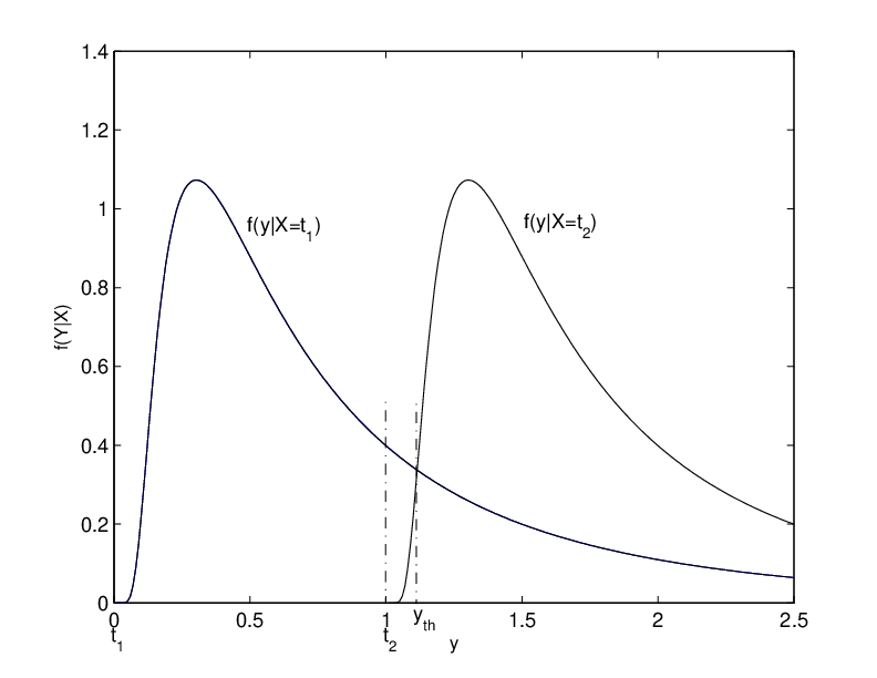
To illustrate this result, consider Fig. 5: $\delta$ is the area under the curve $f(y|X=t_{1})$ as $y$ varies from $t_{2}$ to $y_{th}$ and is always larger than $\int_{t_{2}}^{y_{th}}f_{Y}(y|X=t_{2})dy$ , the area under the curve $f_{Y}(y|X=t_{2})$ from $t_{2}$ to $y_{th}$ .

This bound can easily be generalized to $T$ -ary modulation. When $X\in\{t_{1},\ldots,t_{T}\},0\leq t_{1}<t_{2},\ldots<t_{T}$ and $p_{1}\geq p_{2}\geq\ldots\geq p_{T}$ , the upper bound on symbol error probability is given by

P_{e}<\sum_{i=1}^{T-1}p_{i}\left(1-F_{N}\left(t_{i+1}-t_{i}\right)\right).

(39)

To compute the ML estimate, the receiver needs to know $\mu$ and $\lambda$ , the parameters of the noise. One way to enable the receiver to acquire the knowledge of these parameters is by training as in a conventional communication system. Appendix C provides the ML estimates of these parameters based on the IG pdf.

IV-C Improving Reliability: Transmitting Multiple Molecules

The performance of a molecular communication system (the mutual information and the error rate performance) can be improved by transmitting multiple molecules to convey a message symbol. We assume that the trajectories of the molecules are independent and they do not interact with each other during their propagation from the transmitter to the receiver.

The transmitter releases $M>1$ molecules simultaneously to convey one of $T$ messages, $X\in\{t_{1},\ldots,t_{T}\}$ . In [9], it was shown using simulations that if multiple molecules are available, releasing them simultaneously is the best strategy. Essentially, releasing them at different times leads to confusion at the receiver with molecules potentially arriving out of order. In the case of simultaneous transmissions, the receiver observes $M$ mutually independent arrival times

Y_{j}=X+N_{j},~j=1,\ldots,M,

(40)

where $N_{j}$ are i.i.d. with $N_{j}\sim{\mathrm{IG}}(\mu,\lambda),j=1,\ldots,M$ .

IV-C1 Maximum likelihood estimation

We first consider ML detection of the symbol when multiple molecules are used. Assuming that the receiver knows the values of $\mu$ and $\lambda$ through an earlier training phase, it can use the multiple observations $Y_{j},j=1,\ldots,M,$ to obtain $\hat{X}_{\text{ML}}$ .

The pdfs $f_{Y_{j}|X}(y_{j}|X=t_{i}),j=1,\ldots,M,$ are i.i.d. with $f_{Y_{j}|X}(y_{j}|X=t_{i})$ given by (21). The ML estimate, in this case, is given by

	$\displaystyle\hat{X}_{\text{ML}}=$	$\displaystyle\arg\max_{t_{i}}\prod_{j=1}^{M}f_{Y_{j}\|X}(y_{j}\|X=t_{i})$
	$\displaystyle=$	$\displaystyle\arg\max_{t_{i}}\prod_{j=1}^{M}(y_{j}-t_{i})^{-3/2}\exp\left(-\frac{\lambda}{2\mu^{2}}\sum_{j=1}^{M}\frac{((y_{j}-t_{i})-\mu)^{2}}{(y_{j}-t_{i})}\right),\hskip 21.68121pty_{j}>t_{i}.$		(41)

Simplifying the above equation, the ML estimate can be expressed as

\hat{X}_{\text{ML}}=\arg\max_{t_{i}}\Lambda_{M}(t_{i})

(42)

where

\Lambda_{M}(t_{i})=-\frac{3}{2}\sum_{j=1}^{M}\log(y_{j}-t_{i})-\frac{\lambda}{2\mu^{2}}\sum_{j=1}^{M}\frac{((y_{j}-t_{i})-\mu)^{2}}{(y_{j}-t_{i})},\hskip 21.68121pty_{j}>t_{i}.

(43)

IV-C2 Linear filter

The above approach estimates the transmitted message using a complicated ML detection filter that processes the received signal. Given the potential applications of this research, a simpler filter would be useful. One such filter is the linear average, which is optimal in an AWGN channel [29]. In this case, the receiver averages the $M$ observations and performs a ML estimate with the sample mean as the test statistic. The receiver generates

Z=\frac{1}{M}\sum_{j=1}^{M}Y_{j}.

(44)

The linear filter has the following nice property: by the additivity property of IG distribution in Property 2, $Z\sim{\mathrm{IG}}(E[X]+\mu,M\lambda)$ . Now,

\hat{X}_{\text{ML}}=\arg\max_{t_{i}}f_{Z}(z|X=t_{i}),

where

f_{Z|X}(z|X=t_{i})=\sqrt{\frac{M\lambda}{2\pi(z-t_{i})^{3}}}\mathrm{exp}\left(-\frac{M\lambda}{2\mu^{2}}\frac{((z-t_{i})-\mu)^{2}}{(z-t_{i})}\right),z>t_{i}.

(45)

The linear receiver therefore acts as if the diffusion constant, $\sigma^{2}$ , is reduced by a factor of $M$ to $\sigma^{2}/M$ . At reasonably high velocities, this leads to better performance; however, we have seen in Section III that, at low velocities, diffusion can actually help communications.

At high drift velocities the reduction in the effective diffusion results in an effect akin to the diversity order in wireless communication systems. This is shown in the following result.

Theorem 4

As drift velocity $v\rightarrow\infty$ ,

\log(P_{e})<-C_{1}\frac{cv^{2}}{\sigma^{2}}+C_{2}+C_{3}\log{\frac{cv^{2}}{\sigma^{2}}},

(46)

where $C_{1},C_{2}$ and $C_{3}$ are constants.

Proof: The proof is found in Appendix D.

Furthermore, for $M$ molecules and detection using the linear filter,

\log(P_{e})<-C_{1}\frac{Mcv^{2}}{\sigma^{2}}+C_{2}+C_{3}\log{\frac{Mcv^{2}}{\sigma^{2}}},

(47)

which is essentially (46) with $\sigma^{2}$ replaced by $\sigma^{2}/M$ .

Since, in both (46) and (47), the first term dominates at high velocities, a semi-log plot of $P_{e}$ versus velocity is asymptotically linear, with slope proportional to $-M$ .

IV-D Simulation Results

Figure 6 shows how the variance and the mean of the ML estimate vary with velocity for a given $\sigma^{2}$ . With increasing velocity, the estimator becomes unbiased and the variance approaches zero. As in Section III, velocity appears to be close to the AIGN equivalent of SNR in AWGN channels; however, again, this is only true at high velocities. At low velocities, both the velocity and the diffusion constant play a role.

Figure 7 plots the symbol error probability with $T$ -ary modulation for different values $T$ . The input alphabet employed for simulations is $X\in\{1+\frac{i-1}{T-1},i=1,\ldots,T\}$ . The figure also compares the upper bound on error probability, presented in Section IV-B, with the error probability obtained through Monte Carlo simulations. The rapidly deteriorating error probability is clear, as is the tightness of the upper bound.

The poor performance of $T$ -ary modulation as shown in Fig. 7 motivates the multiple molecule system described in Section IV-C. Figure 8 plots the error rate performance when $X\in\{1,2\}$ and each symbol is conveyed by releasing multiple molecules. As expected, there is a effect akin to receive diversity in a wireless communication system. Here, the performance gain in the error probability increases with the number of molecules transmitted per message symbol.

Figure 8 also compares the performance of the averaging filter with the ML estimation given by (42). The linear averaging filter is clearly suboptimal with performance worsening with increasing number of molecules transmitted per symbol ( $M$ ). This result again underlines the significant differences between the AIGN and AWGN channel models.

V Discussion and Conclusions

In proposing a new channel model based on IG noise, we have necessarily analyzed the simplest possible interesting cases. In this regard, there are several issues left unresolved.

Single versus Multiple Channel Uses: Throughout this paper, we have focused on the case of a single channel use, in which we use the channel to transmit a single symbol of information; our capacity results are measured in units of nats per channel use. Translating these results to nats per molecule is straightforward: each channel use consists of a deterministic number of molecules $M$ , where $M\geq 1$ , thus, we merely divide by $M$ . However, measuring nats per unit time is a more complicated issue, since the duration of the channel use is a random variable, dependent on both the input and the output. Following [19], where the capacity per unit time of a queue timing channel was calculated with respect to the average service time, here we can normalize our capacity results either with the average propagation time $E[N]$ , or the average length of the communication session $E[Y]$ . Since $E[Y]=E[X]+E[N]$ , our decision to constrain the mean of the input distribution $f_{X}(x)$ would then have a natural interpretation in terms of the capacity per unit time.

Further, our system model excludes the possibility of other molecules propagating in the environment, except those transmitted as a result of the channel use; equivalently, we assume each channel use is orthogonal. This raises the question of how to use the channel repeatedly: if the signalling molecules are indistinguishable, then (under our formulation) the transmitter must wait until all $M$ molecules have arrived before a new channel use can begin. On the other hand, if the signalling molecules are distinguishable, then channel uses can take place at any time, or even the same time. This is because, if there is no ambiguity in matching received molecules to channel uses, those channel uses are orthogonal.

Inter-symbol Interference: Repeated channel uses also leads to a situation akin to inter-symbol interference (ISI) in conventional communications. Since propagation time is not bounded, the transmitter may release the molecule corresponding to the “next” symbol while the “previous” molecule is still in transit. Molecules may, therefore, arrive out of order. This problem is exacerbated if multiple molecules are released simultaneously to achieve diversity. Decoding with such ISI is complex since schemes such as the Viterbi algorithm cannot be used (even ignoring the fact that the system would, in theory, have infinite memory). This is because, in each time slot, the number of molecules not yet received - due to transmission from previous time slots - acts as the state of the channel with corresponding noise distributions. In other contexts, an example of a channel with states is the Gilbert-Elliott channel [30].

Synchronization and Differential Encoding: The system model and the analysis presented here assumes perfect synchronization between the transmitter and the receiver. It is unclear how difficult, or easy, it would be to achieve this with nano-scale devices. An information theoretic analysis of the effect of asynchronism in AWGN channels has been presented in [31]. Given the importance of timing in our model, extensions of such work to the AIGN channel would be useful. An interesting alternative would be to use differential modulation schemes such as interval modulation presented in [32].

Amplitude and Timing Modulation: The work presented here focuses on timing modulation, which leads naturally to the AIGN channel model. A more sophisticated scheme would be to use “amplitude” modulation as well - such as by varying the number of molecules released. It may be possible to leverage work on positive-only channels such as in optics [33]. Amplitude modulation could be coupled with the timing modulation considered here. However, it is important to note that any amplitude information would reproduced at the receiver faithfully since, in the model we have considered so far, the receiver is allowed to wait for all molecules to arrive before decoding. Therefore, to be useful, a reasonable model of amplitude modulation must also include receiver imperfections and account for the issue of ISI as described above.

Two-way Communication and Negative Drifts: The AIGN channel model is valid only in the case of a positive drift velocity. In this regard, it does not support two-way communication between nano-devices. With zero drift velocity, the mean transition time is unbounded, but the probability that the molecule arrives approaches 1; with negative drift velocities, even this arrival is not guaranteed [24]. Molecular communications with negative drift velocities remains a completely open problem and one that is outside the scope of this paper. In this case, the noise term is ${\mathrm{IG}}(-\mu,\lambda)$ and the IG framework provided here may be used to analyze such a problem.

In conclusion, our results both illustrate the feasibility of molecular communication and show that it can be given a mathematical framework. However, our results lead to many interesting open questions, some of which are described above. We believe our key contribution here has been to provide this mathematical framework, making it possible to tackle some of these problems.

Appendix A Differential entropy of the IG distribution

Here we prove Property 1. For a given $\mu$ and $\lambda$ , the differential entropy of the noise $h(N)$ is fixed and can be computed from the generalized IG distribution (GIG). The GIG distribution is characterized by three parameters and the pdf of a random variable $X$ distributed as GIG is given by [24]

f_{X}(x;\gamma,\mu,\lambda)=\frac{1}{2\mu^{\gamma}K_{\gamma}\left(\frac{\lambda}{\mu}\right)}~x^{\gamma-1}\exp\left(-\frac{\lambda x^{-1}+(\lambda/\mu^{2})x}{2}\right),\\ -\infty<\gamma<\infty,\mu>0,\lambda\geq 0,x>0,

(48)

where $K_{\gamma}(\cdot)$ is the modified Bessel function of the third kind of order $\gamma$ . It is commonly denoted as ${\mathrm{GIG}}(\gamma,\mu,\lambda)$ and ${\mathrm{IG}}(\mu,\lambda)$ is a special case, obtained by substituting $\gamma=-1/2$ [24].

When $X\sim{\mathrm{GIG}}(\gamma,\mu,\lambda)$ , its differential entropy, in nats, is given by [34]

h(X)=\log\left(2K_{\gamma}(\lambda/\mu)\mu\right)-(\gamma-1)\frac{\frac{\partial}{\partial\gamma}K_{\gamma}(\lambda/\mu)}{K_{\gamma}(\lambda/\mu)}+\frac{\lambda}{2\mu}\frac{K_{\gamma+1}(\lambda/\mu)+K_{\gamma-1}(\lambda/\mu)}{K_{\gamma}(\lambda/\mu)}.

(49)

Setting $\gamma=-1/2$ , the differential entropy of $N\sim{\mathrm{IG}}(\mu,\lambda)$ is given by

h(N)=h_{\text{IG}(\mu,\lambda)}=\log\left(2K_{-1/2}(\lambda/\mu)\mu\right)+\frac{3}{2}\frac{\frac{\partial}{\partial\gamma}K_{\gamma}(\lambda/\mu)\left|{}_{\gamma=-1/2}\right.}{K_{-1/2}(\lambda/\mu)}+\frac{\lambda}{2\mu}\frac{K_{1/2}(\lambda/\mu)+K_{-3/2}(\lambda/\mu)}{K_{-1/2}(\lambda/\mu)},

(50)

and the property follows.

Appendix B Evaluating optimal input distribution at low velocities

If a pdf exists that leads to an exponentially distributed measured signal $Y$ , it would be the capacity achieving input distribution. Furthermore, the pdf of the measured signal is the convolution of the pdf of the input and that of IG noise pdf. We therefore attempt to evaluate the optimal distribution at asymptotically low velocities by deconvolving the known optimal distribution (exponential) of the output $Y$ and the IG noise. The Laplace transform of the IG distribution is given by

\mathcal{L}(N)=E[e^{-sX}]=\exp\left[\frac{\lambda}{\mu}\left(1-\sqrt{1+\frac{2\mu^{2}}{\lambda}s}\right)\right].

(51)

For given values of $\sigma^{2}$ and $d$ , as $v\rightarrow 0$ , $\mu\rightarrow\infty$ and $\gamma$ is fixed. In such a case, $\mathcal{L}(N)$ can be approximated as

\mathcal{L}(N)\approx\exp\left(-\sqrt{2\lambda s}\right).

(52)

As $Y=X+N$ , $\mathcal{L}(X)=\mathcal{L}(Y)/\mathcal{L}(N)$ . To achieve the upper bound on capacity, $f_{Y}(y)=\frac{1}{m_{Y}}e^{\frac{-y}{m_{Y}}}$ , where $m_{Y}=E[Y]=E[X]+\mu$ and hence

\mathcal{L}(Y)=\frac{1/m_{Y}}{s+(1/m_{Y})}\Rightarrow\mathcal{L}(X)=\frac{1/m_{Y}}{(1/m_{Y})+s}\exp\left(\sqrt{2\lambda s}\right)

(53)

and the pdf of $X$ can be obtained by computing the inverse Laplace transform $\mathcal{L}^{-1}(X)$ . The inverse Laplace transform can be computed by making use of the following Laplace transform pair [35]:

\mathcal{L}^{-1}\left\{\frac{\exp(-c\sqrt{s+b})}{s-a}\right\}=\frac{e^{at}}{2}\left(\exp\left(-c\sqrt{a+b}\right)\text{erfc}\left(\frac{c}{2\sqrt{t}}-\sqrt{(a+b)t}\right)\right.\\ \left.+\exp\left(c\sqrt{a+b}\right)\text{erfc}\left(\frac{c}{2\sqrt{t}}+\sqrt{(a+b)t}\right)\right),

(54)

where $a,b$ and $c$ are constants. Using(54), we obtain

\mathcal{L}^{-1}\left\{\frac{1/m_{Y}}{s+(1/m_{Y})}\exp(\sqrt{2\lambda}\sqrt{s})\right\}=\frac{(1/m_{Y})e^{\frac{-1}{m_{Y}t}}}{2}\left(\exp\left(\jmath\sqrt{2\lambda/m_{Y}}\right)\text{erfc}\left(-\sqrt{\lambda/2t}-\jmath\sqrt{t/m_{Y}}\right)\right.\\ \left.+\exp\left(-\jmath\sqrt{2\lambda/m_{Y}}\right)\text{erfc}\left(-\sqrt{\lambda/2t}+\jmath\sqrt{t/m_{Y}}\right)\right)

(55)

where

\text{erfc}(z)=\frac{2}{\sqrt{\pi}}\int_{z}^{\infty}e^{-z^{2}}dz

Note that $\text{erfc}(z)$ can be evaluated for complex values of its argument $z$ and $\text{erfc}(z^{*})=(\text{erfc}(z))^{*}$ , where $z^{*}$ is the complex conjugate of $z$ . Hence

f_{X}(x)=\frac{e^{\frac{-1}{m_{Y}x}}}{m_{Y}}\Re\left\{\exp\left(\jmath\sqrt{2\lambda/m_{Y}}\right)\text{erfc}\left(-\sqrt{\lambda/2x}-\jmath\sqrt{x/m_{Y}}\right)\right\}.

(56)

This, unfortunately, does not appear to be a valid pdf. The capacity of the AIGN channel at low velocities is therefore, yet, unknown.

B-A When there is no drift

To confirm the result in (56), we test the case of zero velocity. Note that in this case, the noise is not IG; however, the zero velocity case converges in limit to the case without drift. Without drift, the arrival time has a pdf given by [24],

f(t)=\sqrt{\frac{\lambda}{2\pi t^{3}}}\mathrm{exp}^{\frac{-\lambda}{2t}},\hskip 36.135ptt>0

(57)

Note that $t\sim\mbox{Inverse Gamma}(1/2,\lambda/2)$ . The inverse Gamma distribution, with shape parameter $\alpha$ and scale parameter $\beta$ , is given by

f(t;\alpha,\beta)=\frac{\beta^{\alpha}}{\Gamma(\alpha)}(1/t)^{\alpha+1}\mathrm{exp}(\beta/t),~t>0.

(58)

Hence, the Laplace transform of the inverse Gamma distribution is

\mathcal{L}(N)=\mathcal{L}[InvGamma(1/2,\lambda/2)]=\frac{2(s\lambda/2)^{1/4}}{\sqrt{\pi}}K_{1/2}(\sqrt{2\lambda s}).

(59)

Substituting

K_{1/2}(z)=\sqrt{\frac{\pi}{2z}}e^{-z},

(60)

we get

\mathcal{L}(N)=e^{-\sqrt{2\lambda s}}

(61)

This results in

\mathcal{L}(X)=\frac{1/m_{Y}}{s+(1/m_{Y})}e^{\sqrt{2\lambda s}}

(62)

Note that (61) is same as (52) and (62) is same as (53). Hence, we get (56) when we try to obtain $f_{X}(x)$ by evaluating $\mathcal{L}^{-1}(X)$ .

Appendix C Estimating Noise Parameters

To estimate the noise parameters, the transmitter releases $k$ “training” molecules at known time $t_{0}$ . Let the receiver observe $Y_{j}=t_{0}+N_{j},j=1,2,\ldots,k,$ where $N_{j}\sim{\mathrm{IG}}(\mu,\lambda)$ are i.i.d. and the receiver knows $t_{0}$ a priori. The pdf’s of $(Y_{j}-t_{0}),j=1,\ldots,k$ , are i.i.d. and IG distributed as given by

f_{Y_{j}-t_{0}}(y_{j}-t_{0})=\sqrt{\frac{\lambda}{2\pi(y_{j}-t_{0})^{3}}}\exp\left(-\frac{\lambda}{2\mu^{2}}\frac{((y_{j}-t_{0})-\mu)^{2}}{(y_{j}-t_{0})}\right),y_{j}>t_{0}.

(63)

In general, $\infty<t_{0}<-\infty$ ; however, in our case, $0<t_{0}<\infty$ . When $Y\sim{\mathrm{IG}}(t_{0},\mu,\lambda)$ , $m_{Y}=E[Y]=\mu+t_{0}$ . When the receiver knows the value of $t_{0}$ , the ML estimates of the remaining two parameters $\mu$ and $\lambda$ can be obtained as

\hat{\mu}(t_{0})=\bar{Y}-t_{0},

(64)

where $\bar{Y}=\frac{1}{k}\sum_{j=1}^{k}Y_{j}$ is the sample mean and

\hat{\lambda}(t_{0})=\left[\frac{1}{k}\sum_{j=1}^{k}\left(\frac{1}{Y_{j}-t_{0}}-\frac{1}{\bar{Y}-t_{0}}\right)\right]^{-1}.

(65)

Assuming $\mu$ and $\lambda$ does not change significantly from the time the receiver estimates the parameters and the time of actual communication, the receiver can obtain the ML estimate of the release times of the molecules.

Appendix D Upper Bound on Asymptotic Error Rate

Here we prove Theorem 4. Recall that, for $2$ -ary modulation with $X\in\{t_{1},t_{2}\},0\geq t_{1}\geq t_{2}$ , the upper bound on SEP is given by

P_{e}<p_{1}(1-F_{N}(t_{2}-t_{1})).

(66)

where

F_{N}(n)=\Phi\left(\sqrt{\frac{\lambda}{n}}\left(\frac{n}{\mu}-1\right)\right)+e^{2\lambda/\mu}\Phi\left(-\sqrt{\frac{\lambda}{n}}\left(\frac{n}{\mu}+1\right)\right)

(67)

where $\Phi(z)=\frac{1}{2}\left(1+\text{erf}\left(\frac{z}{\sqrt{2}}\right)\right)$ is the cdf of a standard Gaussian distributed random variable $Z$ . Here,

\text{erf}(z)=\frac{2}{\sqrt{\pi}}\int_{0}^{z}e^{-u^{2}}du

(68)

For $z\gg 1$ , $\text{erf}(z)$ can be approximated as

\text{erf}(z)\approx 1-\frac{e^{-z^{2}}}{\sqrt{\pi}z}

(69)

Now, we compute $F_{N}(c)$ , $c=t_{2}-t_{1}$ , and examine its behavior as $v\rightarrow\infty$ . Recall that $\mu=\frac{d}{v}$ and $\lambda=\frac{d^{2}}{\sigma^{2}}$ .

F_{N}(c)=\Phi\left(\sqrt{\frac{cv^{2}}{\sigma^{2}}}-\sqrt{\frac{d^{2}}{c\sigma^{2}}}\right)+e^{2vd/\sigma^{2}}\Phi\left(-\sqrt{\frac{cv^{2}}{\sigma^{2}}}-\sqrt{\frac{d^{2}}{c\sigma^{2}}}\right)

(70)

Consider the first term in $F_{N}(c)$ .

\Phi\left(\sqrt{\frac{cv^{2}}{\sigma^{2}}}-\sqrt{\frac{d^{2}}{c\sigma^{2}}}\right)=\frac{1}{2}\left(1+\text{erf}\left(\frac{\sqrt{\frac{cv^{2}}{\sigma^{2}}}-\sqrt{\frac{d^{2}}{c\sigma^{2}}}}{\sqrt{2}}\right)\right)

(71)

When $v\rightarrow\infty$ , $\sqrt{\frac{cv^{2}}{\sigma^{2}}}\rightarrow\infty$ and thus $\left(\sqrt{\frac{cv^{2}}{\sigma^{2}}}-\sqrt{\frac{d^{2}}{c\sigma^{2}}}\right)\gg 1$ . Hence, we use the approximation given by (69) to obtain

\Phi\left(\sqrt{\frac{cv^{2}}{\sigma^{2}}}-\sqrt{\frac{d^{2}}{c\sigma^{2}}}\right)\approx 1-\frac{1}{\sqrt{2\pi}}\frac{1}{\sqrt{\frac{cv^{2}}{\sigma^{2}}}-\sqrt{\frac{d^{2}}{c\sigma^{2}}}}e^{\left(-\frac{cv^{2}}{\sigma^{2}}+\frac{2vd}{\sigma^{2}}-\frac{d^{2}}{c\sigma^{2}}\right)}

(72)

Now, consider the second term in $F_{N}(c)$ .

\Phi\left(-\sqrt{\frac{cv^{2}}{\sigma^{2}}}-\sqrt{\frac{d^{2}}{c\sigma^{2}}}\right)=\frac{1}{2}\left(1-\text{erf}\left(\frac{\sqrt{\frac{cv^{2}}{\sigma^{2}}}+\sqrt{\frac{d^{2}}{c\sigma^{2}}}}{\sqrt{2}}\right)\right)

(73)

When $v\rightarrow\infty$ $\left(\sqrt{\frac{cv^{2}}{\sigma^{2}}}+\sqrt{\frac{d^{2}}{c\sigma^{2}}}\right)\gg 1$ and, using the approximation given by (69), we obtain

e^{2vd/\sigma^{2}}\Phi\left(-\sqrt{\frac{cv^{2}}{\sigma^{2}}}-\sqrt{\frac{d^{2}}{c\sigma^{2}}}\right)\approx\frac{1}{\sqrt{2\pi}}\frac{1}{\sqrt{\frac{cv^{2}}{\sigma^{2}}}+\sqrt{\frac{d^{2}}{c\sigma^{2}}}}e^{\left(-\frac{cv^{2}}{\sigma^{2}}-\frac{d^{2}}{c\sigma^{2}}\right)}

(74)

Hence,

F_{N}(c)\approx 1-\frac{1}{\sqrt{2\pi}}\frac{1}{\sqrt{\frac{cv^{2}}{\sigma^{2}}}-\sqrt{\frac{d^{2}}{c\sigma^{2}}}}e^{\left(-\frac{cv^{2}}{\sigma^{2}}+\frac{2vd}{\sigma^{2}}-\frac{d^{2}}{c\sigma^{2}}\right)}+\frac{1}{\sqrt{2\pi}}\frac{1}{\sqrt{\frac{cv^{2}}{\sigma^{2}}}+\sqrt{\frac{d^{2}}{c\sigma^{2}}}}e^{\left(-\frac{cv^{2}}{\sigma^{2}}-\frac{d^{2}}{c\sigma^{2}}\right)}

(75)

As $e^{\left(-\frac{cv^{2}}{\sigma^{2}}-\frac{d^{2}}{c\sigma^{2}}\right)}$ decays faster than $e^{\left(-\frac{cv^{2}}{\sigma^{2}}+\frac{2vd}{\sigma^{2}}-\frac{d^{2}}{c\sigma^{2}}\right)}$ , the second term in the above equation dominates the rate at which $F_{N}(c)$ goes to $1$ as $v\rightarrow\infty$ . At high velocities, $F_{N}(c)$ can be approximated as

F_{N}(c)\approx 1-\frac{1}{\sqrt{2\pi}}\frac{e^{-\frac{cv^{2}}{\sigma^{2}}}}{\sqrt{\frac{cv^{2}}{\sigma^{2}}}}

(76)

Thus, at high velocities, the upper bound on SEP is given by $\frac{1}{\sqrt{2\pi}}\frac{e^{-\frac{cv^{2}}{\sigma^{2}}}}{\sqrt{\frac{cv^{2}}{\sigma^{2}}}}$ . The theorem follows by taking the logarithm of this expression.

References

[1] S. F. Bush, Nanoscale Communication Networks. Boston: Artech House, 2010.
[2] S. Hiyama et al., “Molecular communication,” in Proc. 2005 NSTI Nanotechnology Conference, 2005, pp. 391–394.
[3] T. Nakano, T. Suda, M. Moore, R. Egashira, A. Enomoto, and K. Arima, “Molecular communication for nanomachines using intercellular calcium signaling,” in Nanotechnology, 2005. 5th IEEE Conference on, Jul. 2005, pp. 478–481.
[4] Y. Moritani, S. M. Nomura, S. Hiyama, K. Akiyoshi, and T. Suda, “A molecular communication interface using liposomes with gap junction proteins,” in Bio-Inspired Models of Network, Information and Computing Systems, 2006. 1st, Dec. 2006.
[5] M. Moore, A. Enomoto, T. Nakano, R. Egashira, T. Suda, A. Kayasuga, H. Kojima, H. Sakakibara, and K. Oiwa, “A design of a molecular communication system for nanomachines using molecular motors,” in Pervasive Computing and Communications Workshops, 2006. PerCom Workshops 2006. Fourth Annual IEEE International Conference on, Mar. 2006.
[6] S. Hiyama, Y. Moritani, and T. Suda, “A biochemically engineered molecular communication system,” in 3rd International Conference on Nano-Networks, Boston, MA, 2008.
[7] S. Hiyama and Y. Moritani, “Molecular communication: Harnessing biochemical materials to engineer biomimetic communication systems,” Nano Communication Networks, vol. 1, pp. 20–30, Mar. 2010.
[8] A. W. Eckford, “Molecular communication: Physically realistic models and achievable information rates,” IEEE Trans. Inf. Theory, submitted for publication. arXiv:0812.1554v1 [cs.IT] 8 December 2008.
[9] S. Kadloor and R. S. Adve, “Development of a framework to study a molecular communication system,” in Proc. of the 18th International Conf. on Computer Comm. and Networks, 2009.
[10] S. Kadloor, R. S. Adve, and A. W. Eckford, “Molecular communication using Brownian motion with drift,” IEEE Trans. Nanobioscience, submitted for publication. arXiv:1006.3959v1 [physics.bio-ph].
[11] M. J. Moore, T. Suda, and K. Oiwa, “Molecular communication: Modeling noise effects on information rate,” IEEE Transactions on Nanobioscience, vol. 8, pp. 169–179, Jun 2009.
[12] B. Atakan and O. Akan, “An information theoretical approach for molecular communication,” in Proc. 2nd Intl. Conf. on Bio-Inspired Models of Network, Information, and Computing Systems, Budapest, Hungary, 2007, pp. 33–40.
[13] M. Pierobon and I. F. Akyildiz, “A physical end-to-end model for molecular communication in nanonetworks,” IEEE J. Sel. Areas in Commun., vol. 28, no. 4, pp. 602–611, May 2010.
[14] P. Thomas, D. Spencer, S. Hampton, P. Park, and J. Zurkus, “The diffusion mediated biochemical signal relay channel,” Adv. Neural Inform. Process. Syst., vol. 16, pp. 1263–1270, 2004.
[15] B. Atakan and O. B. Akan, “Single and multiple-access channel capacity in molecular nanonetworks,” in 4th International Conference on Nano-Networks, Luzern, Switzerland, 2009.
[16] T. Nakano and J.-Q. Liu, “Design and analysis of molecular relay channels: An information theoretic approach,” IEEE Transactions on Nanobioscience, vol. 9, no. 3, pp. 213–221, Sep. 2010.
[17] D. Blackwell, “Information theory,” Modern mathematics for the engineer: Second series, pp. 183–193, 1961.
[18] H. Permuter, P. Cuff, B. V. Roy, and T. Weissman, “Capacity of the trapdoor channel with feedback,” IEEE Transactions on Information Theory, vol. 54, no. 7, pp. 3150–3165, Jul. 2008.
[19] V. Anantharam and S. Verdú, “Bits through queues,” IEEE Trans. Inf. Theory, vol. 42, pp. 4–18, Jan 1996.
[20] R. Sundaresan and S. Verdú, “Capacity of queues via point-process channels,” IEEE Trans. Inf. Theory, vol. 52, pp. 2697–2709, Jun 2006.
[21] S. Goldstein, “Mechanical models of Brownian motion,” Lecture Notes in Physics, vol. 153, pp. 21–24, 1982.
[22] J. Berthier, Microfluidics for Biotechnology. Boston: Artech House, 2006.
[23] I. Karatzas and S. E. Shreve, Brownian Motion and Stochastic Calculus (2nd edition). New York: Springer, 1991.
[24] R. S. Chhikara and J. L. Folks, The Inverse Gaussian Distribution: Theory, Methodology, and Applications. New York: Marcel Dekker, Inc., 1989.
[25] V. Seshadri, The Inverse Gaussian Distribution: Statistical theory and Applications. New York: Springer, 1999.
[26] Y. A. Brychkov and K. A. Geddes, “On the derivatives of the Bessel and Struve functions with respect to the order,” Integral Transforms and Special Functions, vol. 16, pp. 187–198, Apr 2005.
[27] T. M. Cover and J. A. Thomas, Elements of Information Theory. New Jersey: John Wiley & Sons, Inc., 2006.
[28] W. Schwarz, “On the convolution of inverse Gaussian and exponential random variables,” Communications in Statistics: Theory and Methods, vol. 31, pp. 2113–2121, Dec 2002.
[29] J. G. Proakis and M. Salehi, Digital Communications, 5th ed. McGraw-Hill Publishers, 2008.
[30] A. Eckford, F. Kschischang, and S. Pasupathy, “Analysis of low-density parity-check codes for the Gilbert-Elliott channel,” IEEE Transactions on Information Theory, vol. 51, no. 11, pp. 3872 – 3889, November 2005.
[31] A. Tchamkerten, V. Chandar, and G. W. Wornell, “Communication under strong asynchronism,” IEEE Transactions on Information Theory, vol. 55, no. 10, pp. 4508–4528, Oct. 2009.
[32] S. Mukhtar and J. Bruck, “Interval modulation coding,” in Proceedings of IEEE International Symposium on Information Theory, 2002., June 2002, p. 327.
[33] S. Hranilovic and F. Kschischang, “Capacity bounds for power- and band-limited optical intensity channels corrupted by Gaussian noise,” IEEE Transactions on Information Theory, vol. 50, no. 5, pp. 784 – 795, May 2004.
[34] T. Kawamura and K. Iwase, “Characterizations of the distributions of power inverse Gaussian and others based on the entropy maximization principle,” J. Japan Statist. Soc, vol. 33, pp. 95–104, 2003.
[35] R. B. Hetnarski, “An algorithm for generating inverse Laplace transforms of exponential form,” Journal of Applied Mathematics and Physics, vol. 26, pp. 249–253, Mar 1975.