Extended Bayesian Information Criteria for Gaussian Graphical Models

In the sequel we make no distinction between the edge set $\mathbf{E}$ of a graph on $p$ nodes and the associated Gaussian graphical model. Without loss of generality we assume a zero mean vector for all distributions in the model. We also refer to $\mathbf{E}$ as a set of entries in a $p\times p$ matrix, meaning the $2|\mathbf{E}|$ entries indexed by $(j,k)$ and $(k,j)$ for each $\{j,k\}\in\mathbf{E}$. We use $\Delta$ to denote the index pairs $(j,j)$ for the diagonal entries of the matrix.

Let $\Theta_{0}$ be a positive definite matrix supported on $\Delta\cup\mathbf{E}_{0}$. In other words, the non-zero entries of $\Theta_{0}$ are precisely the diagonal entries as well as the off-diagonal positions indexed by $\mathbf{E}_{0}$; note that a single edge in $\mathbf{E}_{0}$ corresponds to two positions in the matrix due to symmetry. Suppose the random vectors $X_{1},\dots,X_{n}$ are independent and distributed identically according to $N(0,\Theta_{0}^{-1})$. Let $S=\frac{1}{n}\sum_{i}X_{i}X_{i}^{T}$ be the sample covariance matrix. The Gaussian log-likelihood function simplifies to

We introduce some further notation. First, we define the maximum variance of the individual nodes:

Next, we define $\theta_{0}=\min_{\mathbf{e}\in\mathbf{E}_{0}}|(\Theta_{0})_{\mathbf{e}}|$, the minimum signal over the edges present in the graph. (For edge $\mathbf{e}=\{j,k\}$, let $(\Theta_{0})_{\mathbf{e}}=(\Theta_{0})_{jk}=(\Theta_{0})_{kj}$.) Finally, we write $\lambda_{\max}$ for the maximum eigenvalue of $\Theta_{0}$. Observe that the product $\sigma^{2}_{\max}\lambda_{\max}$ is no larger than the condition number of $\Theta_{0}$ because $1/\lambda_{\min}(\Theta_{0})=\lambda_{\max}(\Theta_{0}^{-1})\geq\sigma^{2}_{\max}$.

Suppose that $n$ tends to infinity with the following asymptotic assumptions on data and model:

Here $C,\kappa>0$ and $\gamma$ are fixed reals, while the integers $p,q$, the edge set $\mathbf{E}_{0}$, the matrix $\Theta_{0}$, and thus the quantities $\sigma^{2}_{\max}$, $\lambda_{\max}$ and $\theta_{0}$ are implicitly allowed to vary with $n$. We suppress this latter dependence on $n$ in the notation. The ‘big oh’ $\mathbf{O}(\cdot)$ and the ‘small oh’ $\mathbf{o}(\cdot)$ are the Landau symbols.

In order to prove this theorem we use two techniques for comparing likelihoods of different models. Firstly, in Chen and Chen’s work on the GLM case [6], the Taylor approximation to the log-likelihood function is used and we will proceed similarly when comparing the smallest true model $\mathbf{E}_{0}$ to models $\mathbf{E}$ which do not contain $\mathbf{E}_{0}$. The technique produces a lower bound on the decrease in likelihood when the true model is replaced by a false model.

Secondly, Porteous [8] shows that in the case of two nested models which are both decomposable, the likelihood ratio (at the maximum likelihood estimates) follows a distribution that can be expressed exactly as a log product of Beta distributions. We will use this to address the comparison between the model $\mathbf{E}_{0}$ and decomposable models $\mathbf{E}$ containing $\mathbf{E}_{0}$ and obtain an upper bound on the improvement in likelihood when the true model is expanded to a larger decomposable model.

Some details on the proofs of Theorems 1 and 2 are given in Section 5.

In our simulations, we examine the EBIC as applied to the case where the graph is a chain with node $j$ being connected to nodes $j-1,j+1$, and to the ‘double chain’, where node $j$ is connected to nodes $j-2,j-1,j+1,j+2$. Figure 1 shows examples of the two types of graphs, which have on the order of $p$ and $2p$ edges, respectively. For both the chain and the double chain, we investigate four different scaling scenarios, with the exponent $\kappa$ selected from $\{0.5,0.9,1,1.1\}$. In each scenario, we test $n=100,200,400,800$, and define $p\propto n^{\kappa}$ with the constant of proportionality chosen such that $p=10$ when $n=100$ for better comparability.

In the case of a chain, the true inverse covariance matrix $\Theta_{0}$ is tridiagonal with all diagonal entries $(\Theta_{0})_{j,j}$ set equal to 1, and the entries $(\Theta_{0})_{j,j+1}=(\Theta_{0})_{j+1,j}$ that are next to the main diagonal equal to 0.3. For the double chain, $\Theta_{0}$ has all diagonal entries equal to 1, the entries next to the main diagonal are $(\Theta_{0})_{j,j+1}=(\Theta_{0})_{j+1,j}=0.2$ and the remaining non-zero entries are $(\Theta_{0})_{j,j+2}=(\Theta_{0})_{j+2,j}=0.1$. In both cases, the choices result in values for $\theta_{0}$, $\sigma^{2}_{\max}$ and $\lambda_{\max}$ that are bounded uniformly in the matrix size $p$.

For each data set generated from $N(0,\Theta_{0}^{-1})$, we use the ‘glasso’ package [2] in R to compute the ‘glasso path’. We choose 100 penalty values $\rho$ which are logarithmically evenly spaced between $\rho_{\max}$ (the smallest value which will result in a no-edge model) and $\rho_{\max}/100$. At each penalty value $\rho$, we compute $\hat{\Theta}_{\rho}$ from (4) and define the model $\mathbf{E}_{\rho}$ based on this estimate’s support. The R routine also allows us to compute the unpenalized maximum likelihood estimate $\hat{\Theta}(\mathbf{E}_{\rho})$. We may then readily compute the EBIC from (1). There is no guarantee that this procedure will find the model with the lowest EBIC along the full ‘glasso path’, let alone among the space of all possible models of size $\leq q$. Nonetheless, it serves as a fast way to select a model without any manual tuning.

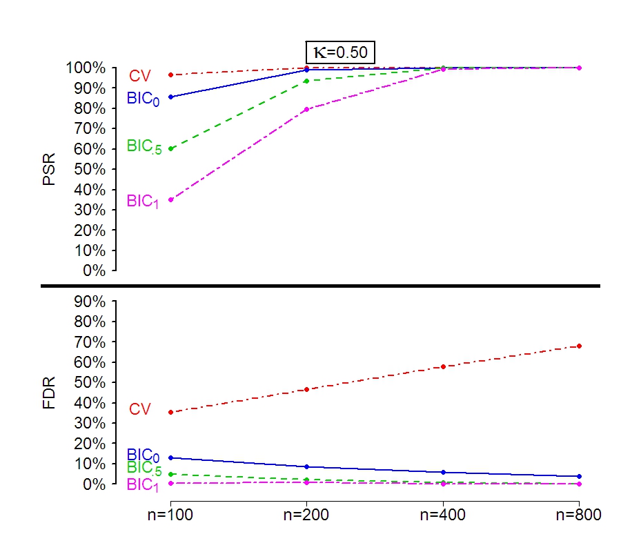
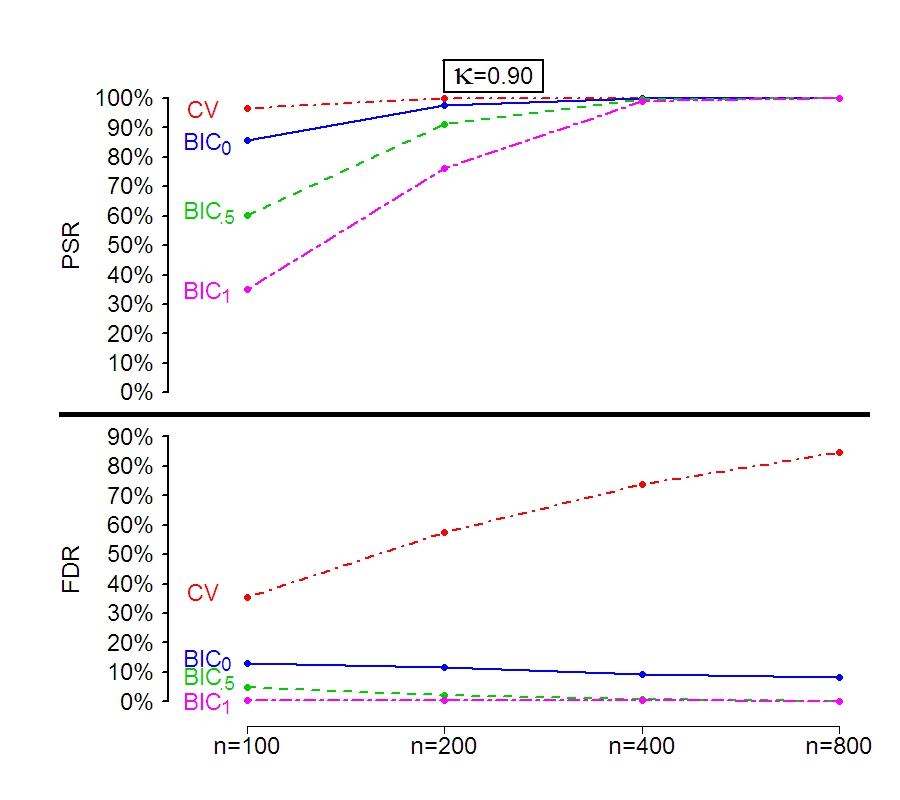
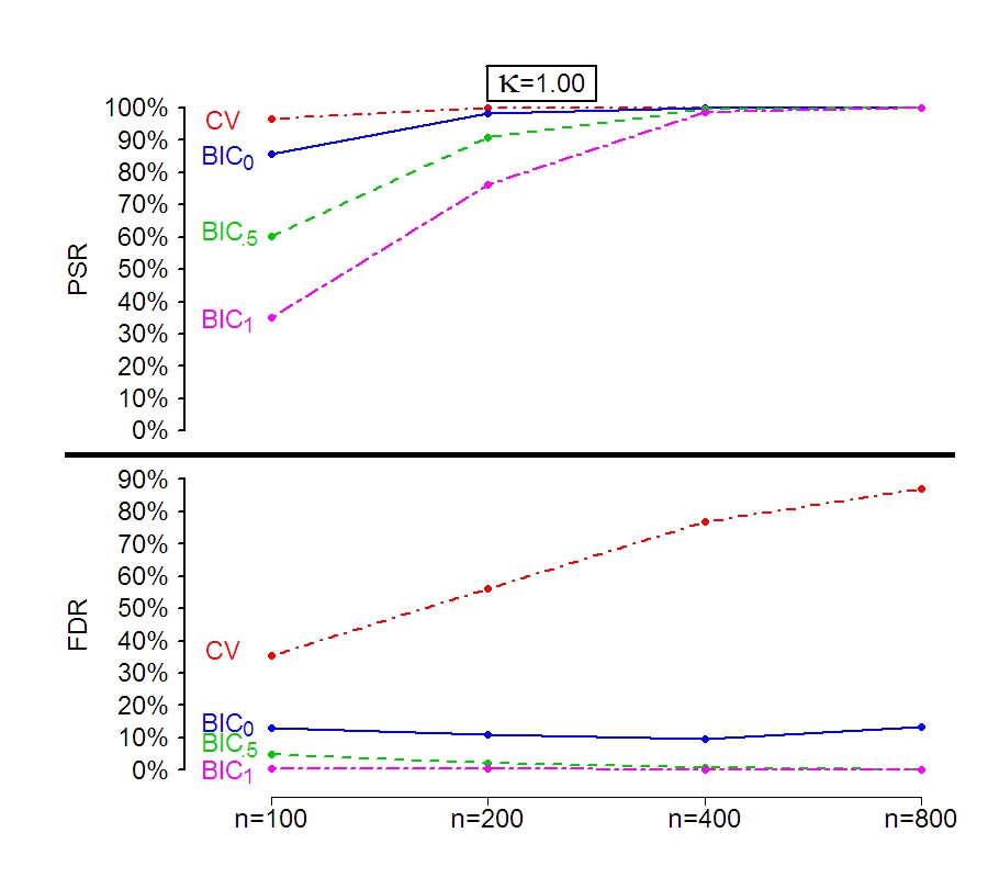
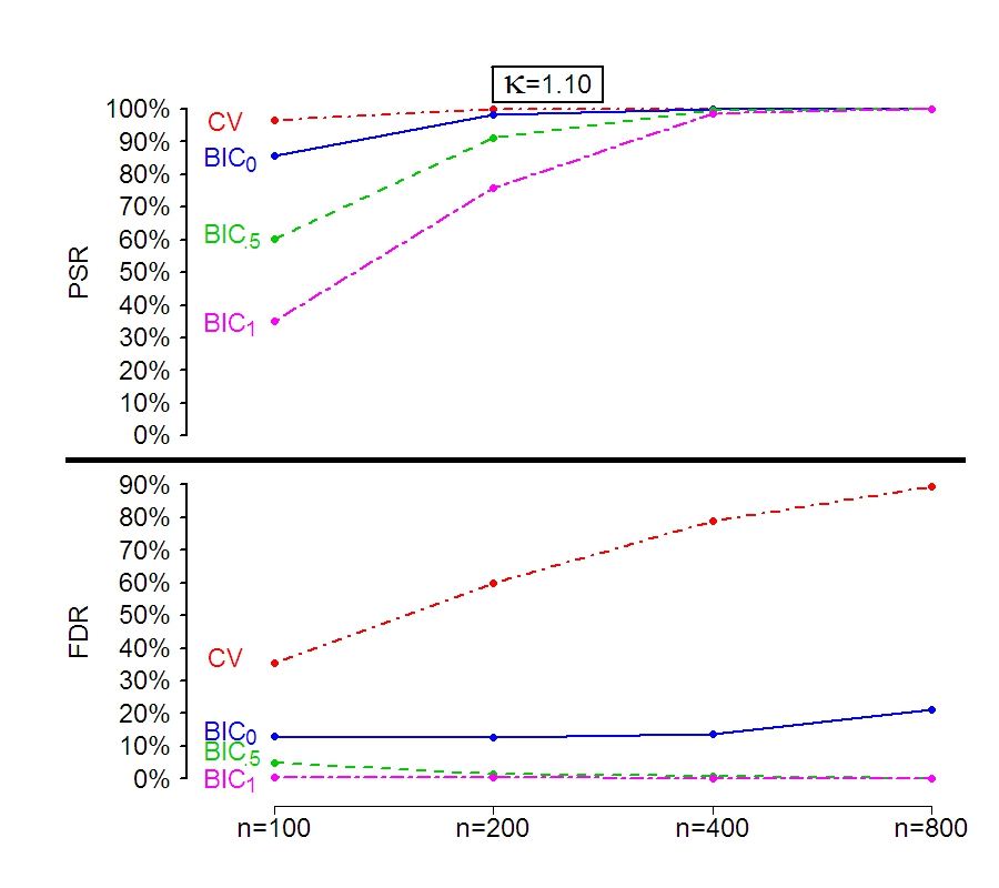
Chain graph: The results for the chain graph are displayed in Figure 2. The figure shows the positive selection rate (PSR) and false discovery rate (FDR) in the four scaling scenarios. We observe that, for the larger sample sizes, the recovery of the non-zero coefficients is perfect or nearly perfect for all three values of $\gamma$; however, the FDR rate is noticeably better for the positive values of $\gamma$, especially for higher scaling exponents $\kappa$. Therefore, for moderately large $n$, the EBIC with $\gamma=0.5$ or $\gamma=1$ performs very well, while the ordinary $\mathrm{BIC}_{0}$ produces a non-trivial amount of false positives. For 100-fold cross-validation, while the PSR is initially slightly higher, the growing FDR demonstrates the extreme inconsistency of this method in the given setting.

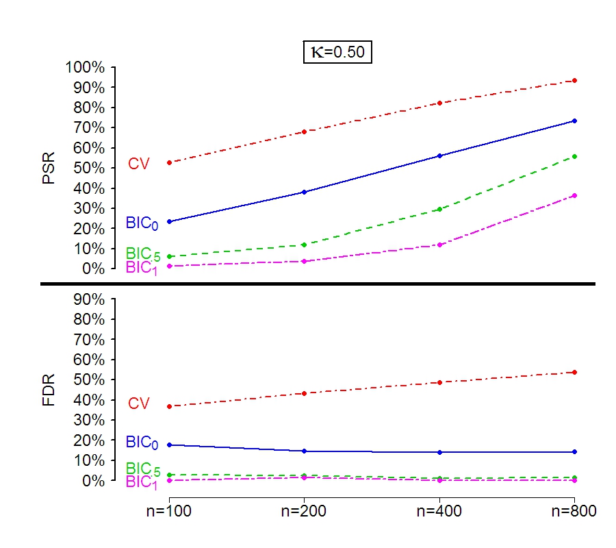
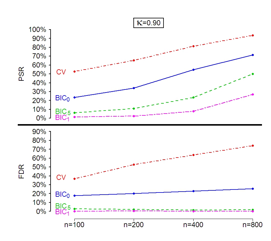
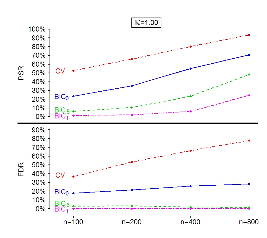
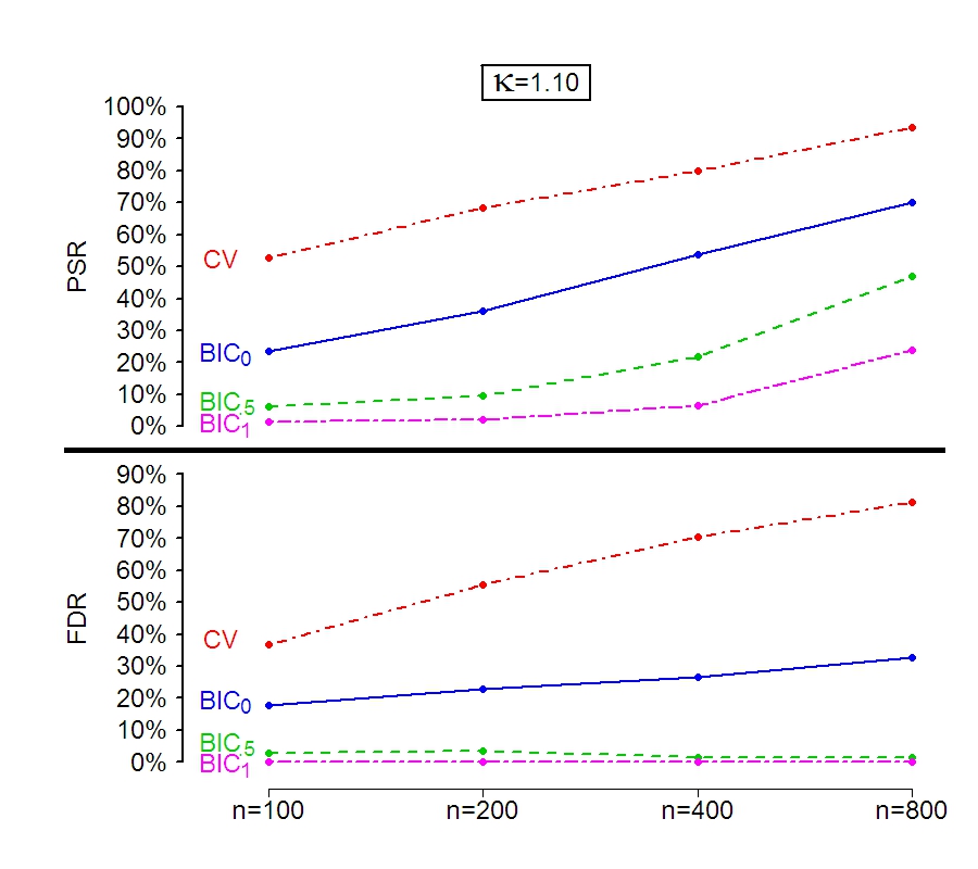
Double chain graph: The results for the double chain graph are displayed in Figure 3. In each of the four scaling scenarios for this case, we see a noticeable decline in the PSR as $\gamma$ increases. Nonetheless, for each value of $\gamma$, the PSR increases as $n$ and $p$ grow. Furthermore, the FDR for the ordinary $\mathrm{BIC}_{0}$ is again noticeably higher than for the positive values of $\gamma$, and in the scaling scenarios $\kappa\geq 0.9$, the FDR for $\mathrm{BIC}_{0}$ is actually increasing as $n$ and $p$ grow, suggesting that asymptotic consistency may not hold in these cases, as is supported by our theoretical results. 100-fold cross-validation shows significantly better PSR than the BIC and EBIC methods, but the FDR is again extremely high and increases quickly as the model grows, which shows the unreliability of cross-validation in this setting. Similarly to what Chen and Chen [3] conclude for the regression case, it appears that the EBIC with parameter $\gamma=0.5$ performs well. Although the PSR is necessarily lower than with $\gamma=0$, the FDR is quite low and decreasing as $n$ and $p$ grow, as desired.

For both types of simulations, the results demonstrate the trade-off inherent in choosing $\gamma$ in the finite (non-asymptotic) setting. For low values of $\gamma$, we are more likely to obtain a good (high) positive selection rate. For higher values of $\gamma$, we are more likely to obtain a good (low) false discovery rate. (In the proofs given in Section 5, this corresponds to assumptions (5) and (6)). However, asymptotically, the conditions (3) guarantee consistency, meaning that the trade-off becomes irrelevant for large $n$ and $p$. In the finite case, $\gamma=0.5$ seems to be a good compromise in simulations, but the question of determining the best value of $\gamma$ in general settings is an open question. Nonetheless, this method offers guaranteed asymptotic consistency for (known) values of $\gamma$ depending only on $n$ and $p$.

We begin by stating two lemmas that are used in the proof of the main result, but are also more generally interesting as tools for precise bounds on Gaussian and chi-square distributions. First, Cai [10, Lemma 4] proves the following chi-square bound. For any $n\geq 1,\lambda>0$,

We can give an analagous left-tail upper bound. The proof is similar to Cai’s proof and omitted here. We will refer to these two bounds together as (CSB).

Second, we give a distributional result about the sample correlation when sampling from a bivariate normal distribution.

We assume the following two conditions, where $\epsilon_{0},\epsilon_{1}>0$, $C\geq\sigma^{2}_{\max}\lambda_{\max}$, $\kappa=\log_{n}p$, and $\gamma_{0}=\gamma-(1-\frac{1}{4\kappa})$:

We are now ready to give a non-asymptotic version of the Main Theorem. For its proof apply the union bound to the statements in Theorems 3 and 4, as in the asymptotic proof given in section 2.

Finally, we note that translating the above to the asymptotic version of the result is simple. If the conditions (3) hold, then for sufficiently large $n$ (and thus sufficiently large $p$), assumptions (5) and (6) hold. Furthermore, although we may not have the exact equality $\kappa=\log_{n}p$, we will have $\log_{n}p\rightarrow\kappa$; this limit will be sufficient for the necessary inequalities to hold for sufficiently large $n$. The proofs then follow from the non-asymptotic results.

References

- [1] Steffen L. Lauritzen. Graphical models, volume 17 of Oxford Statistical Science Series. The Clarendon Press Oxford University Press, New York, 1996. Oxford Science Publications.
- [2] Jerome Friedman, Trevor Hastie, and Robert Tibshirani. Sparse inverse covariance estimation with the graphical lasso. Biostatistics, 9(3):432–441, 2008.
- [3] Jiahua Chen and Zehua Chen. Extended Bayesian information criterion for model selection with large model space. Biometrika, 95:759–771, 2008.
- [4] Gideon Schwarz. Estimating the dimension of a model. Ann. Statist., 6(2):461–464, 1978.
- [5] Malgorzata Bogdan, Jayanta K. Ghosh, and R. W. Doerge. Modifying the Schwarz Bayesian information criterion to locate multiple interacting quantitative trait loci. Genetics, 167:989–999, 2004.
- [6] Jiahua Chen and Zehua Chen. Extended BIC for small--large- sparse GLM. Preprint.
- [7] Pradeep Ravikumar, Martin J. Wainwright, Garvesh Raskutti, and Bin Yu. High-dimensional covariance estimation by minimizing -penalized log-determinant divergence. arXiv:0811.3628, 2008.
- [8] B. T. Porteous. Stochastic inequalities relating a class of log-likelihood ratio statistics to their asymptotic distribution. Ann. Statist., 17(4):1723–1734, 1989.
- [9] Jun Shao. Linear model selection by cross-validation. J. Amer. Statist. Assoc., 88(422):486–494, 1993.
- [10] T. Tony Cai. On block thresholding in wavelet regression: adaptivity, block size, and threshold level. Statist. Sinica, 12(4):1241–1273, 2002.
- [11] P. Svante Eriksen. Tests in covariance selection models. Scand. J. Statist., 23(3):275–284, 1996.
Appendix A Appendix
This section gives the proof for Lemma 1, and fills in the details of the proofs of Theorems 3 and 4.
Lemma 1For any , for any ,
Remark 1.
We note that some lower bound on is intuitively necessary in order to be able to bound the ‘left tail’, because the mode of the distribution is at (for ). If is very close to zero, then the ‘left tail’ () actually includes the mode ; therefore, we could not hope to get an exponentially small probability for being in the tail. However, this intuitive explanation suggests that we should have ; perhaps the bound in this lemma could be tightened.
We first prove a preliminary lemma:
Lemma A.1.
For any , for any ,
Proof.
Let denote the density function for , and let denote the density function for . Then, using , we get:
So,
First, note that is an increasing function for , and therefore
(Here the last inequality is from the Taylor series). Next, since is a convex function (where ), and since , we see that
Finally, it is a fact that . Putting the above bounds together, and assuming that , we obtain
Since we require , the quantity in the brackets is at most , and so
Therefore,
∎
Now we prove Lemma 1.
First suppose that is even. Let denote the density function of the distribution. From [10], if ,
Iterating this identity, we get
Now set for . We obtain
By Stirling’s formula,
and so,
This is clearly sufficient to prove the desired bound in the case that is even. Next we turn to the odd case; let be odd. First observe that if , the statement is trivial, while if , then , therefore is positive. By Lemma A.1 and the expression above,
Next we turn to the theorems. Recall assumptions 5 and 6. Lemmas A.2 and A.3 below are sufficient to fill in the details of Theorem 3.
Lemma A.2.
With probability at least , the following holds for all edges in the complete graph:
Fix some edge . Then
Write , , . Then
By Lemma 2, there are some independent such that
There are edges in the complete graph. Therefore, by the union bound, it will suffice to show that, with probability at least ,
Suppose this bound does not hold. Then
Since , this implies that
Since , it will suffice to show that with probability at least ,
Write . Observe that, by assumption (5), and ; therefore (by Taylor series),
Furthermore,
By (CSB) from the paper,
and also,
This gives the desired result.∎
Lemma A.3.
It is sufficient to show that
We rewrite this as
where
Using , it’s sufficient to show that
Dividing out common factors, the above is equivalent to showing that
By assumption (5), we know:
as desired. ∎
Lemma A.4.
First, we show that . By assumption (6) we see that:
Now turn to assumption (5). We see that the right-hand side of (5) is . On the left-hand side of (5), by definition, . Therefore,
Therefore, using the stochastic inequality in the statement in the lemma,
Now we apply the chi-square bound from [10], and obtain that
Since and , we obtain that the upper bound is at most
By assumption (6), we may further bound this expression from above as