跳到论文正文
W Papers独立论文阅读器 arXiv:1011.6631 论文正文 计算阅读时间 · 0%
引用这篇论文根据当前论文元数据生成,正式投稿前建议核对。


License: arXiv.org perpetual non-exclusive license
arXiv:1011.6631v2 [hep-ph] 10 Feb 2011

Antenna subtraction at NNLO with hadronic initial states: double real radiation for initial-initial configurations with two quark flavours

Preprint:  ANL-HEP-PR-10-58
Aude Gehrmann-De Ridder    Mathias Ritzmann Affiliation: Institute for Theoretical Physics, ETH, CH-8093 Zürich, Switzerland
Abstract: 

The antenna subtraction formalism allows to calculate QCD corrections to jet observables. Within this formalism, the subtraction terms are constructed using antenna functions describing all unresolved radiation between a pair of hard radiator partons. In this paper, we focus on the subtraction terms for double real radiation contributions to jet observables in hadron-hadron collisions evaluated at NNLO. An essential ingredient to these subtraction terms are the four-parton antenna functions with both radiators in the initial state. We outline the construction of the double real subtraction terms, classify all relevant antenna functions and describe their integration over the relevant antenna phase space. For the initial-initial antenna functions with two quark flavours, we derive the phase space master integrals and obtain the integrated antennae.

Keywords: 
QCD, Jets, Collider Physics, NLO and NNLO Calculations

1 Introduction

Jet production processes constitute an important tool for precision studies due to their large cross sections at high energy colliders. Reliable theoretical predictions for these observables require the calculation of at least the next-to-leading order QCD corrections. For these observables, the inclusive cross section with two incoming hadrons H1,H2H_{1},H_{2} can be written as

𝑑σ=∑a,b∫d​ξ1​d​ξ2​fa/1​(ξ1)​fb/2​(ξ2)​d​σ^a​b​(ξ1​H1,ξ2​H2),{\rm d}\sigma=\sum_{a,b}\int{\rm d}\xi_{1}{\rm d}\xi_{2}\,f_{a/1}(\xi_{1})\,f_{b/2}(\xi_{2})\,{\rm d}\hat{\sigma}_{ab}(\xi_{1}H_{1},\xi_{2}H_{2})\;, (1)

where ξ1\xi_{1} and ξ2\xi_{2} are the momentum fractions of the partons of species aa and bb in the incoming hadrons, ff being the corresponding parton distribution functions and d​σ^a​b​(ξ1​H1,ξ2​H2){\rm d}\hat{\sigma}_{ab}(\xi_{1}H_{1},\xi_{2}H_{2}) is the parton-level scattering cross section for incoming partons aa and bb.

The partonic cross section d​σ^a​b{\rm d}\hat{\sigma}_{ab} has a perturbative expansion in the strong coupling αs\alpha_{s} such that theoretical predictions for a hadronic process at a given order in αs\alpha_{s} are obtained when all partonic channels contributing to that order of the partonic cross section are summed and convoluted with the appropriate parton distribution functions as in eq. (1).

In general, beyond the leading order, each partonic channel contains both ultraviolet and infrared (soft and collinear) divergences. The ultraviolet poles are removed by renormalisation in each channel. Collinear poles originating from the radiation of initial state partons are cancelled by mass factorisation counterterms and absorbed in the parton distribution functions. The remaining soft and collinear poles cancel among each other when all partonic contributions are summed over [1]. As jet observables depend in a nontrivial manner on the experimental criteria used to define them, they can only be calculated numerically. The computation of hadronic observables including higher order corrections therefore requires a systematic procedure to cancel infrared singularities among different partonic channels before any numerical computation of the observable can be performed.

For the task of next-to-leading order (NLO) calculations, the infrared divergences present in real radiation contributions can be systematically extracted by process-independent procedures, called subtraction methods. The purpose of any subtraction method at NLO is to provide a subtraction term which has the same singular behaviour as the real radiation squared matrix element and is sufficiently simple to be integrated analytically over the radiation phase space which has been factorised from the (m+1)(m+1)-particle phase space. The actual form of this subtraction term depends on the subtraction formalism used. Several successful subtraction formalisms have been proposed in the literature [2, 3, 4, 5, 6]. Most notably, the FKS [3] subtraction by Frixione, Kunszt and Signer and the dipole formalism of Catani and Seymour [2] have been implemented in an automated way, the former in [7], the latter in [8, 9, 10, 11, 12, 13]. The major challenge for NLO calculations is the computation of one-loop amplitudes for multiparticle processes. The evaluations of 2→42\to 4 processes at the next-to-leading order represent the current frontier [14, 15, 16, 17].

Nevertheless, for some hadronic processes, in particular 2→12\to 1 or 2→22\to 2 scattering processes such as Drell-Yan, Higgs production, dijet production, vector-boson plus jet, vector-boson pair production or heavy quark pair production, the accuracy of the next-to-leading order predictions is not sufficient to match the anticipated experimental accuracy, expected to reach the order of a few percent or better. Accurate precision studies enabling the extraction of fundamental parameters of the theory will require that the theoretical predictions have the same precision. Those need therefore to be evaluated up to the next-to-next-to-leading order (NNLO) in perturbative QCD .

The calculation of observables with mm jets in addition to other objects (like for example vector bosons) at the NNLO requires three distinct contributions: the double real radiation d​σ^N​N​L​OR{\rm{d}}\hat{\sigma}_{NNLO}^{R} with (m+2)(m+2) final state partons, the mixed real-virtual radiation d​σ^N​N​L​OV,1{\rm{d}}\hat{\sigma}_{NNLO}^{V,1} with (m+1)(m+1) final state partons and the 2-loop virtual radiation d​σ^N​N​L​OV,2{\rm{d}}\hat{\sigma}_{NNLO}^{V,2}, with mm final state partons. Those build the NNLO cross section which is given by

d​σ^N​N​L​O\displaystyle{\rm d}\hat{\sigma}_{NNLO} =\displaystyle= ∫d​Φm+2d​σ^N​N​L​OR+∫d​Φm+1d​σ^N​N​L​OV,1+∫d​Φmd​σ^N​N​L​OV,2.\displaystyle\int_{{\rm{d}}\Phi_{m+2}}{\rm{d}}\hat{\sigma}_{NNLO}^{R}+\int_{{\rm{d}}\Phi_{m+1}}{\rm{d}}\hat{\sigma}_{NNLO}^{V,1}+\int_{{\rm{d}}\Phi_{m}}{\rm{d}}\hat{\sigma}_{NNLO}^{V,2}. (2)

The individual contributions in the mm-, (m+1)(m+1)- and (m+2)(m+2)-parton final states are all separately infrared divergent. After renormalisation and factorisation, their sum is finite, though. For most massless jet observables of phenomenological interest, the two-loop matrix elements have been computed some time ago, while the one-loop matrix elements are usually known from calculations of NLO corrections to (m+1)(m+1)-jet production [18] . The one-loop and two-loop matrix-elements contain explicit infrared divergences from the loop integration. Those cancel with divergences which are implicit in the real radiation for (m+1)(m+1)- and (m+2)(m+2)-parton processes. These real radiation divergences become explicit only once the phase space integration is carried out. The main issue of these calculations is therefore to find a method to extract and cancel the infrared divergences among these three contributions in order to finally evaluate numerically the finite remainders to obtain the NNLO contribution to the cross section.

Like at NLO, a subtraction formalism is needed in order to extract the infrared divergences from these contributions. At parton level, the general form of the cross section for an mm-particle final state at NNLO including subtraction terms is given by [19]:

d​σ^N​N​L​O\displaystyle{\rm d}\hat{\sigma}_{NNLO} =\displaystyle= ∫d​Φm+2(d​σ^N​N​L​OR−d​σ^N​N​L​OS)+∫d​Φm+2d​σ^N​N​L​OS\displaystyle\int_{{\rm{d}}\Phi_{m+2}}\left({\rm{d}}\hat{\sigma}_{NNLO}^{R}-{\rm{d}}\hat{\sigma}_{NNLO}^{S}\right)+\int_{{\rm{d}}\Phi_{m+2}}{\rm{d}}\hat{\sigma}_{NNLO}^{S} (3)
+\displaystyle+ ∫d​Φm+1(d​σ^N​N​L​OV,1−d​σ^N​N​L​OV​S,1)+∫d​Φm+1d​σ^N​N​L​OV​S,1+∫d​Φm+1d​σ^N​N​L​OM​F,1\displaystyle\int_{{\rm{d}}\Phi_{m+1}}\left({\rm{d}}\hat{\sigma}_{NNLO}^{V,1}-{\rm{d}}\hat{\sigma}_{NNLO}^{VS,1}\right)+\int_{{\rm{d}}\Phi_{m+1}}{\rm{d}}\hat{\sigma}_{NNLO}^{VS,1}+\int_{{\rm{d}}\Phi_{m+1}}{\rm{d}}\hat{\sigma}_{NNLO}^{MF,1}
+\displaystyle+ ∫d​Φmd​σ^N​N​L​OV,2+∫d​Φmd​σ^N​N​L​OM​F,2.\displaystyle\int_{{\rm{d}}\Phi_{m}}{\rm{d}}\hat{\sigma}_{NNLO}^{V,2}+\int_{{\rm{d}}\Phi_{m}}{\rm{d}}\hat{\sigma}_{NNLO}^{MF,2}.

Here, d​σ^N​N​L​OS{\rm d}\hat{\sigma}^{S}_{NNLO} denotes the subtraction term for the (m+2)(m+2)-parton final state which behaves like the double real radiation contribution d​σ^N​N​L​OR{\rm d}\hat{\sigma}^{R}_{NNLO} in all singular limits. Likewise, d​σ^N​N​L​OV​S,1{\rm d}\hat{\sigma}^{VS,1}_{NNLO} is the one-loop virtual subtraction term coinciding with the one-loop (m+1)(m+1)-particle contribution d​σ^N​N​L​OV,1{\rm d}\hat{\sigma}^{V,1}_{NNLO} in all singular limits. The two-loop correction to the mm-parton final state is denoted by d​σ^N​N​L​OV,2{\rm d}\hat{\sigma}^{V,2}_{NNLO}. In addition, when there are partons in the initial state, there are two mass factorisation contributions, d​σ^N​N​L​OM​F,1{\rm d}\hat{\sigma}^{MF,1}_{NNLO} and d​σ^N​N​L​OM​F,2{\rm d}\hat{\sigma}^{MF,2}_{NNLO}, for the (m+1)(m+1)- and mm-particle final states respectively. Like at the next-to-leading order level, the subtraction terms are needed in their unintegrated as well as in their integrated forms.

There have been several approaches to build a general subtraction scheme at NNLO [19, 20, 21, 22, 23, 24, 25, 26, 27, 28, 29]. Another subtraction scheme, the qTq_{T}-subtraction formalism has been proposed in [30]. It has been applied to evaluate observables related to processes with colourless high mass final states [30, 31, 32, 33]. In addition, there is a completely independent approach called sector decomposition which relies on a systematic expansion of the integrals in distributions followed by a purely numerical integration. It has been developed for virtual [34, 35, 36] and real radiation [37, 38, 39, 40] corrections at NNLO, and applied to several observables already [41, 42, 43, 44].

We will follow the NNLO antenna subtraction method which was derived in [19] for decays of a colourless initial state into massless final state partons. This formalism has been applied in the computation of NNLO corrections to three-jet production in electron-positron annihilation [45, 46, 47, 48] and related event shapes [49, 50, 51, 52, 53], which were subsequently used in precision determinations of the strong coupling constant [54, 55, 56, 57, 58].

For processes with initial-state partons, the antenna subtraction formalism has been so far fully worked out only to NLO in [59]. It has been extended to NNLO for processes involving one initial state parton relevant for electron-proton scattering in  [60] while an extension of the formalism to include two initial state hadrons at NNLO is under construction [61, 62]. An essential step towards this aim is performed in [62] where an explicit derivation of the subtraction terms needed for the double real contributions to the six-gluon process is presented. The general structure of the unintegrated subtraction terms relevant for the double real contributions to any hadronic observables evaluated at NNLO is presented there as well.

In this paper, we will focus on the integrated form of the subtraction term relevant for double real radiation for processes involving two partons in the initial state. In the antenna subtraction formalism, the subtraction terms are built with so-called antenna functions. The latter describe all unresolved partonic radiation off a hard pair of colour-ordered partons, the radiators. Depending on where the two hard radiators are located, three cases need to be distinguished: both radiators are in the final state (final-final), only one radiator parton is in the initial state (initial-final) or both radiator partons are in the initial state (initial-initial). The subtraction terms and the antenna functions building them are separated corresponding to these three cases. In the most general hadronic process (two partons in the initial state, two or more partons in the final state), all three configurations have to be taken into account.

As discussed in [19, 60, 62] the subtraction terms are separated according to the colour connection of the unresolved partons. In this paper, we will specialise on the subtraction term for the case where two unresolved (soft or collinear) partons are colour connected to the two incoming partons. This is indeed the only case where new ingredients, namely the four-parton initial-initial antennae are needed in unintegrated as well as in integrated forms. On a longer term we are aiming to evaluate the whole set of integrated four-parton initial-initial antennae, those are universal building blocks for the subtraction terms for any hadronic process evaluated at NNLO.

In a first step towards this aim, in this paper, we have focused on the crossings of two partons from a set of three 4-parton final-final antennae involving two quark flavours. More precisely, the paper will be organised as follows: In Section 2, we present the general formulae for the subtraction terms related to double real radiation for initial-initial configurations while the colour-connected case is treated explicitly in Section 3. Section 4 establishes a list of all non-identical initial-initial four-parton antenna functions relevant to construct the subtraction term for the double real radiation off two initial-state partons. In Section 5, the phase space mapping appropriate for initial-initial configurations is presented.

Finally, Section 6 contains our results for the integrated initial-initial antenna functions with two quark flavours and Section 7 our conclusions. Since the results are lengthy, we show only the leading pole terms in the manuscript, and attach the complete results as a Mathematica file.

2 Antenna subtraction for double-real radiation at NNLO in the initial-initial configuration

Antenna subtraction has been derived explicitly for final-final and initial-final configurations at NLO and NNLO in [19] and in [59, 60] respectively. For the initial-initial case, it has been derived at NLO in [59] and is under construction at NNLO.

At NLO, the subtraction term is introduced to extract and cancel the infrared divergences present in the real contributions. The general forms of the subtraction terms required at NLO in any of the three configurations (final-final, initial-final and initial-initial) have been given in [19, 59] and summarised in [62]. At this order, only tree-level three-parton antenna functions involving one unresolved parton are needed to build the subtraction terms. Those functions are usually denoted by Xi​j​k0X^{0}_{ijk}, Xi,j​k0X^{0}_{i,jk}, Xi​k,j0X^{0}_{ik,j} in the three configurations. Their definitions will be recalled in Section 4.

At NNLO, two contributions, double real and mixed real-virtual, require the introduction of a subtraction term. For final-final and initial-final configurations both types of subtraction terms have been constructed; at this order tree-level four-particle antennae involving two unresolved partons and one-loop three-parton antenna functions are needed respectively. Those functions have been derived and integrated over the corresponding factorised phase space in [19] and [60]. For initial-initial configurations, the general structure of the unintegrated subtraction terms relevant for the double real contributions to p​p→m​jetspp\to m\;\text{jets} is presented in [62], we will recall it in this section.

The double real radiation contribution to the mm-jet cross section in p​ppp collisions reads

d​σ^N​N​L​OR=𝒩​∑m+2d​Φm+2​(k1,…,km+2,p1,p2)​1Sm+2\displaystyle{\rm d}\hat{\sigma}^{R}_{NNLO}={\cal N}\,\sum_{m+2}{\rm d}\Phi_{m+2}(k_{1},\ldots,k_{m+2};p_{1},p_{2})\frac{1}{S_{{m+2}}} (4)
×\displaystyle\times |ℳm+2​(p1,p2,k1,…,km+2)|2​Jm(m+2)​(k1,…,km+2,p1,p2).\displaystyle|{\cal M}_{m+2}(p_{1},p_{2};k_{1},\ldots,k_{m+2})|^{2}\;J_{m}^{(m+2)}(k_{1},\ldots,k_{m+2};p_{1},p_{2})\;.

In this equation, |ℳm+2​(p1,p2,k1,…,km+2)|2|{\cal M}_{m+2}(p_{1},p_{2};k_{1},\ldots,k_{m+2})|^{2} stands for the colour-ordered 2→m+22\rightarrow m+2 matrix-element squared. The symmetry factor Sm+2S_{m+2} accounts for identical partons in the final state. The normalisation factor 𝒩{\cal N} includes all QCD-independent factors as well as the dependence on the renormalised QCD coupling constant αs\alpha_{s}. ∑m+2\sum_{m+2} denotes the sum over all configurations with m+2m+2 partons. The initial state momenta are labelled as usual as p1p_{1} and p2p_{2} whereas the m+2m+2 momenta in the final state are labeled k1,…,km+2k_{1},\ldots,k_{m+2}. d​Φm+2{\rm d}\Phi_{m+2} is the 2→m+22\to m+2 particle phase space

d​Φm+2​(k1,…,km+2,p1,p2)=[d​k1]​…​[d​km+2]​(2​π)d​δd​(p1+p2−k1−…−km+2)\displaystyle{\rm d}\Phi_{m+2}(k_{1},\ldots,k_{m+2};p_{1},p_{2})=\left[{\rm d}k_{1}\right]\ldots\left[{\rm d}k_{m+2}\right](2\pi)^{d}\delta^{d}(p_{1}+p_{2}-k_{1}-\ldots-k_{m+2}) (5)

where we have introduced the abbreviation [d​k1]=(dd−1​k1)/(2​E1​(2​π)d−1)\left[{\rm d}k_{1}\right]=({\rm d}^{d-1}k_{1})/(2E_{1}(2\pi)^{d-1}). The jet function Jm(m+2)​(k1,…,km+2,p1,p2)J_{m}^{(m+2)}(k_{1},\ldots,k_{m+2};p_{1},p_{2}) ensures that out of (m+2m+2) final state partons, an observable with mm jets is built. The incoming parton momenta p1,p2p_{1},p_{2} serve as reference directions to define transverse momenta and rapidities of the jets.

The double real radiation contribution given in eq. (4) can become singular if either one or two final state partons are unresolved (soft or collinear). Consequently, when constructing the corresponding subtraction term d​σ^N​N​L​OS{\rm d}\hat{\sigma}^{S}_{NNLO} in eq. (3), which shall correctly subtract all those single and double unresolved singularities we must distinguish the following configurations according to the colour connection of the unresolved partons:

  • (a)

    One unresolved parton but the experimental observable selects only mm jets.

  • (b)

    Two colour-connected unresolved partons (colour-connected).

  • (c)

    Two unresolved partons that are not colour connected but share a common radiator (almost colour-unconnected).

  • (d)

    Two unresolved partons that are well separated from each other in the colour chain (colour-unconnected).

  • (e)

    Large angle soft gluon radiation.

This separation among subtraction contributions according to colour connection is valid in final-final, initial-final or initial-initial configurations and in any of those the subtraction formulae have a characteristic structure in terms of required antenna functions. This antenna structure has been derived for the final-final and initial-final cases in [19, 60] and in [62] for the initial-initial case.

In here, we focus only on the initial-initial case with the kinematical situation where two unresolved partons are colour-connected to the two incoming partons. This is the only case where new ingredients are needed, namely the initial-initial four-parton antenna functions denoted by Xi​l,j​kX_{il,jk}. The four-particle initial-initial antenna functions will be defined explicitly in Section 4.

3 Subtraction terms for two colour-connected unresolved partons in the initial-initial configuration

When two unresolved partons jj and kk are adjacent and colour-connected to two initial-state partons, the subtraction term related to the double real contribution d​σ^N​N​L​OR{\rm d}\hat{\sigma}^{R}_{NNLO} given in eq. (4) reads :

d​σ^N​N​L​OS,b,(i​i)=𝒩​∑m+2d​Φm+2​(k1,…,km+2,p1,p2)​1Sm+2\displaystyle{\rm d}\hat{\sigma}_{NNLO}^{S,b,(ii)}={\cal N}\,\sum_{m+2}{\rm d}\Phi_{m+2}(k_{1},\ldots,k_{m+2};p_{1},p_{2})\frac{1}{S_{m+2}} (6)
×\displaystyle\times ∑i​l∑j​k(Xi​l,j​k0−Xl,j​k0​Xi​L,K0−Xi,k​j0​XI​l,J0)\displaystyle\,\sum_{il}\sum_{jk}\;\left(X^{0}_{il,jk}-X^{0}_{l,jk}X^{0}_{iL,K}-X^{0}_{i,kj}X^{0}_{Il,J}\right)
×\displaystyle\times |ℳm​(p~I^,p~L^,k~1,…,k~i,k~l,…,k~m+2)|2​Jm(m)​(k~1,…,k~i,k~l,…,k~m+2,p~I^,p~L^),\displaystyle|{\cal M}_{m}(\tilde{p}_{\hat{I}},\tilde{p}_{\hat{L}};\tilde{k}_{1},\dotsc,\tilde{k}_{i},\tilde{k}_{l},\dotsc,\tilde{k}_{m+2})|^{2}\,J_{m}^{(m)}(\tilde{k}_{1},\dotsc,\tilde{k}_{i},\tilde{k}_{l},\dotsc,\tilde{k}_{m+2};\tilde{p}_{\hat{I}},\tilde{p}_{\hat{L}})\;,

where the sum runs over all colour-adjacent pairs j,kj,k and implies that the hard momenta i,li,l are chosen accordingly. Xi​l,j​k0X^{0}_{il,jk} denotes a four-particle tree-level initial-initial antenna function defined explicitly in Section 4. By construction those contain all colour connected double unresolved limits of the 2→m+22\rightarrow m+2 parton matrix element associated with partons jj and kk being unresolved between radiators ii and ll.

However this antenna can also become singular in single unresolved limits associated with jj or kk only where it does not coincide with limits of the matrix element. To ensure that this subtraction term is only active in the double unresolved limits of the real matrix elements squared we remove these single unresolved limits of the four-particle antennae. Those limits are products of two tree-level three-particle antennae, namely products of an initial-final antenna Xa,b​cX_{a,bc} and an initial-initial antenna XA​d,CX_{Ad,C}. In these antennae we have replaced the original hard radiators with new particles, I^\hat{I} and L^\hat{L}. When both radiators are in the initial state as it is the case here, pI^=xi​pip_{\hat{I}}=x_{i}p_{i}, pL^=xl​plp_{\hat{L}}=x_{l}p_{l}. The product of these three-particle antenna functions in d​σ^N​N​L​OS,b,(i​i){\rm d}\hat{\sigma}_{NNLO}^{S,b,(ii)} then subtracts the single unresolved limits of the associated four-particle antenna.

The 2→m2\rightarrow m matrix element |ℳm​(p~I^,p~L^,k~1,…,k~i,k~l,…,k~m+2)|2|{\cal M}_{m}(\tilde{p}_{\hat{I}},\tilde{p}_{\hat{L}};\tilde{k}_{1},\dotsc,\tilde{k}_{i},\tilde{k}_{l},\dotsc,\tilde{k}_{m+2})|^{2}  is evaluated with new on-shell momenta which are Lorentz boosted as a result of the mapping required to ensure factorisation of matrix element and phase space. The NNLO initial-initial mappings have been discussed in [59] and will be recalled in this paper in Section 5.
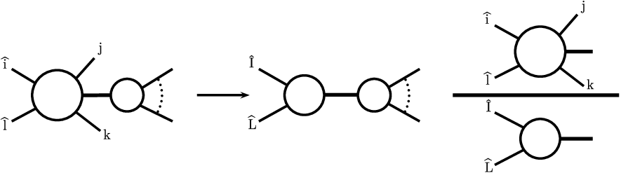
Refer to caption
Figure 1: Illustration of NNLO antenna factorisation representing the factorisation of both the squared matrix elements and the (m+2)(m+2)-particle phase space when the unresolved particles jj and kk are colour connected between two initial state radiators i^\hat{i} and l^\hat{l}.

Using a factorised form for both matrix element and phase space as shown in figure 1, one is able to obtain an integrated form of the subtraction term with mm partons in the final state which can be combined with the virtual two-loop contributions having also mm final state partons as defined in eq. (3).

More explicitly, the factorisation of the phase space with m+2m+2 final state particles denoted by k1,…,km+2k_{1},\ldots,k_{m+2}, reads,

d​Φm+2​(k1,…,km+2,p1,p2)\displaystyle{\rm d}\Phi_{m+2}(k_{1},\ldots,k_{m+2};p_{1},p_{2}) =\displaystyle= d​Φm​(k~1,…,k~i,k~l,…,k~m+2,x1​p1,x2​p2)\displaystyle{\rm d}\Phi_{m}(\tilde{k}_{1},\dotsc,\tilde{k}_{i},\tilde{k}_{l},\dotsc,\tilde{k}_{m+2};x_{1}p_{1},x_{2}p_{2}) (7)
×δ⁡(x1−x^1)​δ​(x2−x^2)​[d​kj]​[d​kk]​d​x1​d​x2.\displaystyle\times\delta(x_{1}-\hat{x}_{1})\,\delta(x_{2}-\hat{x}_{2})\left[{\rm d}k_{j}\right]\left[{\rm d}k_{k}\right]{\rm d}x_{1}{\rm d}x_{2}.

Using this factorised form of the phase space we can rewrite the integrated (colour-connected) subtraction term involving only the four-parton antennae in the form,

|ℳm|2​Jm(m)​d​Φm​∫[d​kj]​[d​kk]​δ​(x1−x^1)​δ​(x2−x^2)​Xi​l,j​k0​d​x1​d​x2.\displaystyle|{\cal M}_{m}|^{2}\,J_{m}^{(m)}\;{\rm d}\Phi_{m}\int\left[{\rm d}k_{j}\right]\left[{\rm d}k_{k}\right]\delta(x_{1}-\hat{x}_{1})\,\delta(x_{2}-\hat{x}_{2})\;X^{0}_{il,jk}{\rm d}x_{1}{\rm d}x_{2}. (8)

Moreover, the integrated antennae are defined as the antenna functions integrated over the antenna phase space as defined in eq. (7) including a normalisation factor to account for powers of the QCD coupling constant by,

𝒳i​l,j​k0​(xi,xl,ε)=1[C⁡(ϵ)]2​∫[d​kj]​[d​kk]​xi​xl​δ​(xi−x^i)​δ​(xl−x^l)​Xi​l,j​k0,\displaystyle{\cal X}^{0}_{il,jk}(x_{i},x_{l},\varepsilon)=\frac{1}{[C(\epsilon)]^{2}}\int\left[{\rm d}k_{j}\right]\left[{\rm d}k_{k}\right]\;x_{i}\;x_{l}\;\delta(x_{i}-\hat{x}_{i})\,\delta(x_{l}-\hat{x}_{l})\,X^{0}_{il,jk},\, (9)

where C⁡(ϵ)C(\epsilon) is given by,

C⁡(ϵ)=(4​π)ϵ​e−ϵ​γ8​π2.C(\epsilon)=(4\pi)^{\epsilon}\frac{e^{-\epsilon\gamma}}{8\pi^{2}}. (10)

These integrations are performed analytically in dd dimensions to make the infrared singularities explicit. The integrated initial-initial antennae are presently unknown and the calculation of a sub-set of those involving two quark flavours is the subject of Section 6 and constitutes our main result in this paper. A list of all non-identical initial-initial four-particle antennae will be presented in Section 4.

4 Initial-initial antenna functions

In this section we shall recall how the antenna functions are defined in any of the configurations and how they enter in the construction of the subtraction terms. We also present a list of all non-identical four-parton initial-initial antenna functions.

4.1 Definitions

In the antenna formalism, in any of the three configurations (final-final, initial-final or initial-initial) the subtraction terms are constructed from products of antenna functions with reduced matrix elements (with fewer final state partons than the original matrix element). The integrated subtraction terms are obtained after an integration over a phase space which is factorised into an antenna phase space (involving all unresolved partons and the two radiators of the antenna) multiplied with a reduced phase space (where the momenta of radiators and unresolved radiation are replaced by two redefined momenta). These redefined momenta can be in the initial state, if the corresponding radiator momenta were in the initial state as we saw in Section 3 in eq. (6) for the subtraction term σN​N​L​OS,b,(i​i)\sigma_{NNLO}^{S,b,(ii)}.

An antenna function is determined by the external states it contains and the pair of hard partons it collapses to in the unresolved limits. In general we denote the antenna function as XX. For antennae that collapse onto a hard quark-antiquark pair, X=AX=A for q​g​q¯qg\bar{q}. Similarly, for a quark-gluon antenna, we have X=DX=D for q​g​gqgg and X=EX=E for q​q′​q¯′qq^{\prime}\bar{q}^{\prime} final states. Finally, we characterise the gluon-gluon antennae as X=FX=F for g​g​gggg, X=GX=G for g​q​q¯gq\bar{q} final states.

At NLO, we only need to consider tree level three-particle antennae involving only one unresolved parton. At NNLO we will need four-particle antennae involving two unresolved partons and one-loop three-particle antennae.

In all cases the antenna functions are derived from physical matrix elements associated to the decay of a colourless particle into partons: the quark-antiquark antenna functions are derived from γ∗→q​q¯+\gamma^{*}\to q\bar{q}~+ (partons) [63], the quark-gluon antenna functions from χ~→g~+\tilde{\chi}\to\tilde{g}~+ (partons)  [64] and the gluon-gluon antenna functions from H→H\to (partons)  [65]. The tree-level antenna functions are obtained by normalising the three- and four-parton tree-level colour sub-amplitudes squared to that of the basic two-parton process: The final-final three- and four-particle antennae are respectively defined by:

Xi​j​k0=Si​j​k,I​K​|ℳi​j​k0|2|ℳI​K0|2,\displaystyle X_{ijk}^{0}=S_{ijk,IK}\,\frac{|{\cal M}^{0}_{ijk}|^{2}}{|{\cal M}^{0}_{IK}|^{2}}\;,
Xi​j​k​l0=Si​j​k​l,I​L​|ℳi​j​k​l0|2|ℳI​L0|2.\displaystyle X_{ijkl}^{0}=S_{ijkl,IL}\,\frac{|{\cal M}^{0}_{ijkl}|^{2}}{|{\cal M}^{0}_{IL}|^{2}}\;. (11)

where SS denotes the symmetry factor associated with the antenna, which accounts both for potential identical particle symmetries and for the presence of more than one antenna in the basic two-parton process. It is chosen such that the antenna function reproduces the unresolved limits of a matrix element with identified particles.

The initial-final tree-level three- and four-parton antennae denoted by Xi,j​k0X_{i,jk}^{0} and Xi,j​k​l0X_{i,jkl}^{0} are in principle obtained by crossing one-parton to the initial state starting from the corresponding final-final antennae. However this crossing might be ambiguous as was first noticed in [59] for the quark-gluon type antenna. Depending on the unresolved limit considered, the pair of hard partons it collapses to may be different.

The initial-initial tree-level three- and four-parton antennae denoted by Xi​k,l0X_{ik,l}^{0} and Xi​l,j​k0X_{il,jk}^{0} are obtained by crossing two partons to the initial state, starting from the final-final antennae. This crossing procedure, unlike in the initial-final case, is free of ambiguity as the pair of hard partons the initial-initial antenna collapses to is always uniquely defined.

More explicitly, the three-parton initial-initial antenna function Xi​k,j0X^{0}_{ik,j} is defined as

Xi​k,j0=Si​j​k,I​K​|ℳ⁡(i^,j,k^)|2|ℳ⁡(I^,K^)|2X^{0}_{ik,j}=S_{ijk,IK}\frac{\left|\mathcal{M}\left(\widehat{i},j,\widehat{k}\right)\right|^{2}}{\left|\mathcal{M}\left(\widehat{I},\widehat{K}\right)\right|^{2}} (12)

where i^\widehat{i} denotes that particle ii is crossed to the initial state. Therefore we can see that the initial-initial antenna is connected to the final-final antenna (where all coloured particles are outgoing) by

Xi​k,j0=(−1)ΔF​X30​(−pi,pj,−pk)X^{0}_{ik,j}=(-1)^{\Delta_{F}}X^{0}_{3}\left(-p_{i},p_{j},-p_{k}\right) (13)

with ΔF\Delta_{F} the difference in the number of fermion crossings between the three-particle and the two-particle subamplitude.

The tree-level four-particle initial-initial antenna Xi​l,j​k0X^{0}_{il,jk} is defined as

Xi​l,j​k0=Si​j​k​l,I​L​|ℳ⁡(i^,j,k,l^)|2|ℳ⁡(I^,L^)|2X^{0}_{il,jk}=S_{ijkl,IL}\frac{\left|\mathcal{M}(\widehat{i},j,k,\widehat{l})\right|^{2}}{\left|\mathcal{M}(\widehat{I},\widehat{L})\right|^{2}} (14)

and the relation to the final-final antenna is

Xi​l,j​k0=(−1)ΔF​X40​(−pi,pj,pk,−pl).X^{0}_{il,jk}=(-1)^{\Delta_{F}}X^{0}_{4}\left(-p_{i},p_{j},p_{k},-p_{l}\right). (15)

The four-particle tree-level antenna functions are not determined by the species of the particles alone but also by the colour-connection. We distinguish leading-colour antennae, denoted by letters without tilde, where the particles are colour-connected in the order they are listed and subleading colour antennae, denoted by letters with tilde, where the gluons are photon-like. This notation has been used in  [19, 60] and we will further use it in this section in the tables below.

The unresolved limits of the initial-initial antennae can be obtained from those of the final-final antennae by crossing. The crossing of the triple-collinear splitting functions is explained in [66]. Those limits will be reported elsewhere.

4.2 Catalogue of tree-level four-particle initial-initial antenna functions

Any two particles of a four-particle final-final antenna can be crossed to the initial state to obtain an initial-initial antenna; therefore one final-final four-particle antenna gives rise to six initial-initial antennae. Due to symmetries, at most four of these initial-initial antennae are different. The independent crossings are listed below. To make the colour connection clear, in this list we write out the arguments of the antennae explicitly, i.e we write X40​(i^,j,k^,l)X^{0}_{4}\left(\widehat{i},j,\widehat{k},l\right) (where i^\widehat{i} denotes an incoming particle) instead of Xi​k,j​l0X^{0}_{ik,jl}. Some initial-initial antennae are free of singular limits. These finite antennae are not needed for the construction of subtraction terms, but their integrated form could be needed for cross-checks. They are marked with ∗⁣∗** below.

quark-antiquark antennae
A40A^{0}_{4} A40​(q^,g^,g,q¯)A^{0}_{4}\big(\widehat{q},\widehat{g},g,\overline{q}\big), A40​(q^,g,g^,q¯)A^{0}_{4}\big(\widehat{q},g,\widehat{g},\overline{q}\big), A40​(q^,g,g,q¯^)A^{0}_{4}\big(\widehat{q},g,g,\widehat{\overline{q}}\big), A40​(q,g^,g^,q¯)A^{0}_{4}\big(q,\widehat{g},\widehat{g},\overline{q}\big)
A~40\widetilde{A}^{0}_{4} A~40​(q^,g^,g,q¯)\widetilde{A}^{0}_{4}\big(\widehat{q},\widehat{g},g,\overline{q}\big), A~40​(q^,g,g,q¯^)\widetilde{A}^{0}_{4}\big(\widehat{q},g,g,\widehat{\overline{q}}\big), A~40​(q,g^,g^,q¯)\widetilde{A}^{0}_{4}\big(q,\widehat{g},\widehat{g},\overline{q}\big)
B40B^{0}_{4} B40​(q^,q′^,q¯′,q¯)B^{0}_{4}\big(\widehat{q},\widehat{q^{\prime}},\overline{q}^{\prime},\overline{q}\big), B40​(q^,q′,q¯′,q¯^)B^{0}_{4}\big(\widehat{q},q^{\prime},\overline{q}^{\prime},\widehat{\overline{q}}\big), B40​(q,q′^,q¯′^,q¯)∗⁣∗B^{0}_{4}\big(q,\widehat{q^{\prime}},\widehat{\overline{q}^{\prime}},\overline{q}\big)^{**}
C40C^{0}_{4} C40​(q^,q¯^,q,q¯)C^{0}_{4}\big(\widehat{q},\widehat{\overline{q}},q,\overline{q}\big), C40​(q^,q¯,q^,q¯)C^{0}_{4}\big(\widehat{q},\overline{q},\widehat{q},\overline{q}\big), C40​(q,q¯^,q^,q¯)∗⁣∗C^{0}_{4}\big(q,\widehat{\overline{q}},\widehat{q},\overline{q}\big)^{**}, C40​(q,q¯,q^,q¯^)∗⁣∗C^{0}_{4}\big(q,\overline{q},\widehat{q},\widehat{\overline{q}}\big)^{**}

A~40​(q^,g,g^,q¯)\widetilde{A}^{0}_{4}\left(\widehat{q},g,\widehat{g},\overline{q}\right) is symmetric under the interchange of the two photon-like gluons. The nonidentical-flavour antenna B40B^{0}_{4} is separately symmetric under interchange of q′q^{\prime} with q¯′\overline{q}^{\prime} and of qq with q¯\overline{q}.

quark-gluon antennae
D40D^{0}_{4} D40​(q^,g^,g,g)D^{0}_{4}\big(\widehat{q},\widehat{g},g,g\big), D40​(q^,g,g^,g)D^{0}_{4}\big(\widehat{q},g,\widehat{g},g\big), D40​(q,g^,g^,g)D^{0}_{4}\big(q,\widehat{g},\widehat{g},g\big), D40​(q,g^,g,g^)D^{0}_{4}\big(q,\widehat{g},g,\widehat{g}\big)
E40E^{0}_{4} E40​(q^,q′^,q¯′,g)E^{0}_{4}\big(\widehat{q},\widehat{q^{\prime}},\overline{q}^{\prime},g\big), E40​(q^,q′,q¯′,g^)E^{0}_{4}\big(\widehat{q},q^{\prime},\overline{q}^{\prime},\widehat{g}\big), E40​(q,q′^,q¯′^,g)E^{0}_{4}\big(q,\widehat{q^{\prime}},\widehat{\overline{q}^{\prime}},g\big), E40​(q,q′^,q¯′,g^)E^{0}_{4}\big(q,\widehat{q^{\prime}},\overline{q}^{\prime},\widehat{g}\big)
E~40\widetilde{E}^{0}_{4} E~40​(q^,q′^,q¯′,g)\widetilde{E}^{0}_{4}\big(\widehat{q},\widehat{q^{\prime}},\overline{q}^{\prime},g\big), E~40​(q^,q′,q¯′,g^)\widetilde{E}^{0}_{4}\big(\widehat{q},q^{\prime},\overline{q}^{\prime},\widehat{g}\big), E~40​(q,q′^,q¯′^,g)\widetilde{E}^{0}_{4}\big(q,\widehat{q^{\prime}},\widehat{\overline{q}^{\prime}},g\big), E~40​(q,q′^,q¯′,g^)\widetilde{E}^{0}_{4}\big(q,\widehat{q^{\prime}},\overline{q}^{\prime},\widehat{g}\big)

Due to the cyclic colour connection, D40D^{0}_{4} is symmetric under interchange of the second and fourth gluon.

gluon-gluon antennae
F40F^{0}_{4} F40​(g^,g^,g,g)F^{0}_{4}\big(\widehat{g},\widehat{g},g,g\big), F40​(g^,g,g^,g)F^{0}_{4}\big(\widehat{g},g,\widehat{g},g\big)
G40G^{0}_{4} G40​(g^,q^,q¯,g)G^{0}_{4}\big(\widehat{g},\widehat{q},\overline{q},g\big), G40​(g^,q,q¯^,g)G^{0}_{4}\big(\widehat{g},q,\widehat{\overline{q}},g\big), G40​(g^,q,q¯,g^)G^{0}_{4}\big(\widehat{g},q,\overline{q},\widehat{g}\big), G40​(g,q^,q¯^,g)G^{0}_{4}\big(g,\widehat{q},\widehat{\overline{q}},g\big)
G~40\widetilde{G}^{0}_{4} G~40​(g^,q^,q¯,g)\widetilde{G}^{0}_{4}\big(\widehat{g},\widehat{q},\overline{q},g\big), G~40​(g^,q,q¯,g^)\widetilde{G}^{0}_{4}\big(\widehat{g},q,\overline{q},\widehat{g}\big), G~40​(g,q^,q¯^,g)\widetilde{G}^{0}_{4}\big(g,\widehat{q},\widehat{\overline{q}},g\big)
H40H^{0}_{4} H40​(q^,q¯^,q′,q¯′)H^{0}_{4}\big(\widehat{q},\widehat{\overline{q}},q^{\prime},\overline{q}^{\prime}\big), H40​(q^,q¯,q′^,q¯′)H^{0}_{4}\big(\widehat{q},\overline{q},\widehat{q^{\prime}},\overline{q}^{\prime}\big)

F40F^{0}_{4} is symmetric under cyclic interchange of its arguments. G~40\widetilde{G}^{0}_{4} is symmetric under the interchange of the two gluons as well as under the interchange of qq with q¯\overline{q}. H40H^{0}_{4} has three symmetries, q↔q¯q\leftrightarrow\overline{q}, q′↔q¯′q^{\prime}\leftrightarrow\overline{q}^{\prime} and the flavour renaming q↔q′q\leftrightarrow q^{\prime}, q¯↔q¯′\overline{q}\leftrightarrow\overline{q}^{\prime}.

5 Phase space factorisation and mappings

The construction of subtraction terms requires a mapping from the original set of momenta onto a reduced set. The mapping interpolates between the different soft and collinear limits which the subtraction term regulates. An appropriate mapping for the initial-initial case, both for single and double unresolved configurations, has been discussed in [59]. By requiring momentum conservation and phase space factorisation, the phase space mapping is strongly constrained. The remapping of initial state momenta can only be a rescaling, since any transversal component would spoil the phase space factorisation. For two unresolved partons jj and kk, a complete factorisation of the phase space into a convolution of an mm-particle phase space depending on redefined momenta only and the phase space of the unresolved partons jj and kk can be achieved with a Lorentz boost. This boost maps the momentum q=p1+p2−kj−kkq\;=\;p_{1}+p_{2}-k_{j}-k_{k} , with q2>0q^{2}>0  and p1,p2p_{1},p_{2} being the momenta of the hard emitters, into the momentum q~=x1​p1+x2​p2\tilde{q}\,=\,x_{1}p_{1}+x_{2}p_{2} , where x1x_{1} and x2x_{2} are fixed in terms of the invariants as follows:

x1\displaystyle x_{1} =\displaystyle= (s12−sj​2−sk​2s12​s12−s1​j−s1​k−sj​2−sk​2+sj​ks12−s1​j−s1​k)12,\displaystyle\left(\frac{s_{12}-s_{j2}-s_{k2}}{s_{12}}\;\frac{s_{12}-s_{1j}-s_{1k}-s_{j2}-s_{k2}+s_{jk}}{s_{12}-s_{1j}-s_{1k}}\right)^{\frac{1}{2}}\,,
x2\displaystyle x_{2} =\displaystyle= (s12−s1​j−s1​ks12​s12−s1​j−s1​k−sj​2−sk​2+sj​ks12−sj​2−sk​2)12.\displaystyle\left(\frac{s_{12}-s_{1j}-s_{1k}}{s_{12}}\;\frac{s_{12}-s_{1j}-s_{1k}-s_{j2}-s_{k2}+s_{jk}}{s_{12}-s_{j2}-s_{k2}}\right)^{\frac{1}{2}}\,. (16)

These two definitions guarantee the overall momentum conservation in the mapped momenta and the correct soft and collinear behaviours . The two momentum fractions x1x_{1} and x2x_{2} satisfy the following limits in double unresolved configurations:

  1. 1.

    jj and kk soft: x1→1x_{1}\rightarrow 1, x2→1x_{2}\rightarrow 1,

  2. 2.

    jj soft and kk=z1​p1k_{k}=z_{1}p_{1}: x1→1−z1x_{1}\rightarrow 1-z_{1}, x2→1x_{2}\rightarrow 1,

  3. 3.

    kj=z1​p1k_{j}=z_{1}p_{1} and kk=z2​p2k_{k}=z_{2}p_{2}: x1→1−z1x_{1}\rightarrow 1-z_{1}, x2→1−z2x_{2}\rightarrow 1-z_{2},

  4. 4.

    kj=z1​p1k_{j}=z_{1}p_{1}, kk=z2​p1k_{k}=z_{2}p_{1}: x1→1−z1−z2x_{1}\rightarrow 1-z_{1}-z_{2}, x2→1x_{2}\rightarrow 1,

and all the limits obtained from the ones above by the exchange of p1p_{1} with p2p_{2} and of kjk_{j} with kkk_{k}. The construction of NNLO antenna subtraction terms also requires that all single unresolved limits of the four-parton initial-initial antenna functions Xi​l,j​kX_{il,jk}, with radiators ii and ll, have to be subtracted, such that the resulting subtraction term is active only in its double unresolved limits. A systematic subtraction of these single unresolved limits by products of two three-parton antenna functions can be performed only if the NNLO phase space mapping turns into an NLO phase space mapping in its single unresolved limits. A detailed discussion of the corresponding translation between these two momentum mappings can be found in [59].

The factorisation of the (m+2)(m+2)-parton phase space into an mm-parton phase space and an antenna phase space involving the unresolved partons jj and kk given in eq. (7) can equivalently be written as

d​Φm+2​(k1,…,km+2,p1,p2)=d​Φm​(k~1,…,k~i,k~l,…,k~m+2,x1​p1,x2​p2)×𝒥δ(q2−x1x2s12)δ(2(x2p2−x1p1).q)×[d​kj]​[d​kk]​d​x1​d​x2,\begin{split}{\rm d}\Phi_{m+2}(k_{1},\ldots,k_{m+2};p_{1},p_{2})&={\rm d}\Phi_{m}(\tilde{k}_{1},\dotsc,\tilde{k}_{i},\tilde{k}_{l},\dotsc,\tilde{k}_{m+2};x_{1}p_{1},x_{2}p_{2})\\ &\quad\times\;{\cal J}\;\delta(q^{2}-x_{1}\,x_{2}\,s_{12})\,\delta(2\,(x_{2}p_{2}-x_{1}p_{1}).q)\,\\ &\quad\times\;[{\rm d}k_{j}]\;[{\rm d}k_{k}]\;{\rm d}x_{1}\;{\rm d}x_{2}\,,\end{split} (17)

where 𝒥{\cal J} is the Jacobian factor defined by

𝒥=s12​(x1​(s12−s1​j−s1​k)+x2​(s12−s2​j−s2​k)).{\cal J}=s_{12}\,\left(x_{1}(s_{12}-s_{1j}-s_{1k})+x_{2}(s_{12}-s_{2j}-s_{2k})\right)\,.

This phase space parametrization can also be used to give an equivalent definition of the integrated initial-initial antennae first given in eq. (9). Those are given as,

𝒳i​l,j​k0​(x1,x2,ε)=1[C⁡(ϵ)]2​∫[d​kj]​[d​kk]​𝒥​x1​x2​δ​(C1)​δ​(C2)​Xi​l,j​k0,{\cal X}^{0}_{il,jk}(x_{1},x_{2},\varepsilon)=\frac{1}{[C(\epsilon)]^{2}}\int[{\rm d}k_{j}][{\rm d}k_{k}]\;{\cal J}\;x_{1}\;x_{2}\;\delta(C_{1})\,\delta(C_{2})\,X^{0}_{il,jk}\,, (18)

where

C1\displaystyle C_{1} =\displaystyle= q2−x1​x2​s12,\displaystyle q^{2}-x_{1}\,x_{2}\,s_{12}\,,
C2\displaystyle C_{2} =\displaystyle= 2​(x2​p2−x1​p1).q.\displaystyle 2(x_{2}p_{2}-x_{1}p_{1}).q\,. (19)

We shall use this definition of the integrated antennae 𝒳i​l,j​k0​(x1,x2,ε){\cal X}^{0}_{il,jk}(x_{1},x_{2},\varepsilon) to compute them in Section 6.

6 Integration of the four-parton initial-initial antennae

In the first part of this section we describe how the initial-initial four-parton antennae are integrated over the antenna phase space while in the second part of this section we restrict ourselves to the evaluation of integrated antennae involving two quark flavours.

6.1 Calculational method

The initial-initial antenna functions have the scattering kinematics

p1+p2→kj+kk+q,p_{1}+p_{2}\to k_{j}+k_{k}+q\;,

where qq is the momentum of the outgoing colourless particle. The momenta satisfy:

p12=p22=0,kj2=kk2=0,q2=q~2=x1​x2​s12.p_{1}^{2}=p_{2}^{2}=0,\;\;k_{j}^{2}=k_{k}^{2}=0,\;\;q^{2}=\tilde{q}^{2}=x_{1}\,x_{2}\,s_{12}\,.

The four-parton initial-initial antennae defined in Section 4 need to be integrated over the phase space of the unresolved partons jj and kk. This integration yields a result which depends only on s12s_{12}, x1x_{1} and x2x_{2}. From dimensional counting, one can immediately conclude that the dependence on s12s_{12} is only multiplicative, according to the mass dimension of the integral.
The initial-initial antenna phase space integrals are derived from squared matrix elements and can be represented by forward scattering diagrams as in the following figure:

[Uncaptioned image]

The two delta functions in eq. (17) can be represented as mass-shell conditions of fake particles and are shown in the previous picture as a thick solid line (representing a massive particle with mass M2=x1​x2​s12M^{2}=x_{1}\,x_{2}\,s_{12}) and a dashed line (representing the other constraint) . This allows us to use the optical theorem to transform the initial-initial antenna phase space integrals into cut two-loop integrals and therefore use the methods developed for multi-loop calculations [67, 68, 69] . Up to eight-propagator integrals with four cut propagators are generated in this way . Using the reduction techniques, the calculation of the integrated antennae can be related to the evaluation of a reduced set of master integrals . For the complete set of non-identical initial-initial four-parton antennae tabulated in Section 4, we find 3232 such integrals, obtained using integration-by-part (IBP, [70]) and Lorentz invariance (LI, [71]) identities, following the Laporta algorithm [72]. A private implementation as well as a public one [73] have been used.
For those four-parton antenna functions there are 1313 different propagators, including the four that are cut in the phase space integration (DjD_{j}, DkD_{k}, Dj​k​12D_{jk12}, Dj​k​123D_{jk123}):

Dj​1\displaystyle D_{j1} =\displaystyle= (p1−kj)2,\displaystyle(p_{1}-k_{j})^{2}\;,
Dk​1\displaystyle D_{k1} =\displaystyle= (p1−kk)2,\displaystyle(p_{1}-k_{k})^{2}\;,
Dj​2\displaystyle D_{j2} =\displaystyle= (p2−kj)2,\displaystyle(p_{2}-k_{j})^{2}\;,
Dk​2\displaystyle D_{k2} =\displaystyle= (p2−kk)2,\displaystyle(p_{2}-k_{k})^{2}\;,
Dj​k\displaystyle D_{jk} =\displaystyle= (kj+kk)2,\displaystyle(k_{j}+k_{k})^{2}\;,
Dj​k​1\displaystyle D_{jk1} =\displaystyle= (p1−kj−kk)2,\displaystyle(p_{1}-k_{j}-k_{k})^{2}\;,
Dj​k​2\displaystyle D_{jk2} =\displaystyle= (p2−kj−kk)2,\displaystyle(p_{2}-k_{j}-k_{k})^{2}\;,
Dj​12\displaystyle D_{j12} =\displaystyle= (p1+p2−kj)2,\displaystyle(p_{1}+p_{2}-k_{j})^{2}\;,
Dk​12\displaystyle D_{k12} =\displaystyle= (p1+p2−kk)2,\displaystyle(p_{1}+p_{2}-k_{k})^{2}\;,
Dj\displaystyle D_{j} =\displaystyle= kj2,\displaystyle k_{j}^{2}\;,
Dk\displaystyle D_{k} =\displaystyle= kk2,\displaystyle k_{k}^{2}\;,
Dj​k​12\displaystyle D_{jk12} =\displaystyle= (p1+p2−kj−kk)2−x1​x2​s12,\displaystyle(p_{1}+p_{2}-k_{j}-k_{k})^{2}-x_{1}x_{2}s_{12}\;,
Dj​k​123\displaystyle D_{jk123} =\displaystyle= (p3+p1+p2−kj−kk)2,\displaystyle(p_{3}+p_{1}+p_{2}-k_{j}-k_{k})^{2}\;, (20)

where p3=x2​p2−x1​p1p_{3}=x_{2}\,p_{2}-x_{1}\,p_{1}. To perform the reduction to master integrals, we drop any integral where DjD_{j}, DkD_{k}, Dj​k​12D_{jk12}, Dj​k​123D_{jk123} are not in the denominator and impose momentum conservation. The integrands of the 3232 master integrals found can all be written as rational polynomials of the denominators above.

These master integrals are calculated using either the method of differential equations or by a direct evaluation of the phase space integrals in terms of hypergeometric functions. The simplest master integral is a two loop bubble with all the internal lines cut, it is obtained from eq. (18) by replacing the jacobian 𝒥\mathcal{J} and the antenna Xi​l,j​k0X^{0}_{il,jk} with unity:

[Uncaptioned image]=I2(x1,x2)=∫ddqddkjddkkδd(p1+p2−q−kj−kk)×\displaystyle\parbox[h]{51.7479pt}{\includegraphics[width=7.76186pt]{PR1noSprod.eps}}\;\;=\,I_{2}(x_{1},x_{2})\,=\,\int d^{d}q\,d^{d}k_{j}\,d^{d}k_{k}\,\delta^{d}\left(p_{1}+p_{2}-q-k_{j}-k_{k}\right)\;\times
δ+(kj2)δ+(kk2)δ+(q2−M2)δ(2(x2p2−x1p1).q).\displaystyle\hskip 113.81102pt\delta^{+}\left(k_{j}^{2}\right)\,\delta^{+}\left(k_{k}^{2}\right)\,\delta^{+}\left(q^{2}-M^{2}\right)\delta(2\,\left(x_{2}p_{2}-x_{1}p_{1}).q\right)\,. (21)

This integral can actually be expressed as a hypergeometric function:

I2=s12−2​ε​(4​π)−4+2​εΓ⁡(2−2​ε)​Γ​(1−ε)2Γ⁡(2−2​ε)​x1−ε​(1−x1)1−2​ε​(1+x1)−εx2−ε​(1−x2)1−2​ε​(1+x2)−ε​(x1+x2)−1+2​εF12​(ε,1−ε,2−2​ε,(1−x1)​(1−x2)(1+x1)​(1+x2)),\begin{split}I_{2}&=s_{12}^{-2\varepsilon}\frac{(4\pi)^{-4+2\varepsilon}}{\Gamma(2-2\varepsilon)}\frac{\Gamma(1-\varepsilon)^{2}}{\Gamma(2-2\varepsilon)}x_{1}^{-\varepsilon}(1-x_{1})^{1-2\varepsilon}(1+x_{1})^{-\varepsilon}\\ &\quad x_{2}^{-\varepsilon}(1-x_{2})^{1-2\varepsilon}(1+x_{2})^{-\varepsilon}(x_{1}+x_{2})^{-1+2\varepsilon}\\ &\quad{}_{2}F_{1}\left(\varepsilon,1-\varepsilon,2-2\varepsilon,\frac{(1-x_{1})(1-x_{2})}{(1+x_{1})(1+x_{2})}\right),\end{split} (22)

it has been checked against the master integral I⁡[0]I[0] appearing in the calculation of the gauge-boson rapidity distribution at NNLO in [68], the notation translates as u=x2/x1u=x_{2}/x_{1}, z=x1​x2z=x_{1}x_{2}.
The set of master integrals which we denote by Ii​(x1,x2,ε){I}_{i}(x_{1},x_{2},\varepsilon) are functions of x1x_{1}, x2x_{2} and ε\varepsilon. We begin by factoring out the leading behavior of the master integrals Ii​(x1,x2,ε)I_{i}(x_{1},x_{2},\varepsilon) in the limits x1→1x_{1}\to 1 and x2→1x_{2}\to 1, keeping the exact ε\varepsilon-dependence:

Ii​(x1,x2,ε)=(1−x1)m1−2​ε​(1−x2)m2−2​ε​ℱi​(x1,x2,ε).{I}_{i}(x_{1},x_{2},\varepsilon)=(1-x_{1})^{m_{1}-2\,\varepsilon}\;(1-x_{2})^{m_{2}-2\,\varepsilon}\;{\cal F}_{i}(x_{1},x_{2},\varepsilon). (23)

The integers m1,m2m_{1},m_{2} are characteristic to each master integral. The functions ℱi​(x1,x2,ε){\cal F}_{i}(x_{1},x_{2},\varepsilon) are regular at x1=1x_{1}=1, at x2=1x_{2}=1, and at x1=x2=1x_{1}=x_{2}\,=1 and can be calculated as Laurent series with, at most, second order poles in ε\varepsilon.

The integrated antennae given by 𝒳⁡(x1,x2,ε){\cal X}(x_{1},x_{2},\varepsilon) are linear combinations of these master integrals Ii​(x1,x2,ε){I}_{i}(x_{1},x_{2},\varepsilon), with coefficients containing poles in ε\varepsilon, as well as in (1−x1)(1-x_{1}) and (1−x2)(1-x_{2}). After the masters have been inserted into the integrated antennae, those take the form

𝒳⁡(x1,x2,ε)=(1−x1)−1−2​ε​(1−x2)−1−2​ε​ℛ​(x1,x2,ε).{\cal X}(x_{1},x_{2},\varepsilon)=(1-x_{1})^{-1-2\,\varepsilon}(1-x_{2})^{-1-2\,\varepsilon}\;{\cal R}(x_{1},x_{2},\varepsilon). (24)

where ℛ⁡(x1,x2,ε){\cal R}(x_{1},x_{2},\varepsilon) is regular at the boundaries x1=1x_{1}=1, x2=1x_{2}=1, and at x1=x2=1x_{1}=x_{2}=1. The ε\varepsilon-expansion of the singular factors (1−xi)−1−2​ε(1-x_{i})^{-1-2\varepsilon} is done in the form of distributions:

(1−xi)−1−2​ε=−12​ε​δ​(1−xi)+∑n(−2​ε)nn!​𝒟n​(xi),(1-x_{i})^{-1-2\varepsilon}\,=\,-\frac{1}{2\varepsilon}\,\delta(1-x_{i})+\sum_{n}\frac{(-2\varepsilon)^{n}}{n!}\mathcal{D}_{n}(x_{i})\,, (25)

with

𝒟n​(xi)=(lnn⁡(1−xi)1−xi)+.\mathcal{D}_{n}(x_{i})=\left(\frac{\ln^{n}\left(1-x_{i}\right)}{1-x_{i}}\right)_{+}\,. (26)

To evaluate the integrated antennae, we decompose the phase space into four regions depending on the values of x1x_{1} and x2x_{2}. Those regions are given by:

  • •

    x1≠ 1x_{1}\,\neq\,1,  x2≠ 1x_{2}\,\neq\,1, which we refer to as the hard region

  • •

    x1= 1x_{1}\,=\,1,  x2≠ 1x_{2}\,\neq\,1, and x1≠ 1x_{1}\,\neq\,1,  x2= 1x_{2}\,=\,1, referred to as collinear regions

  • •

    x1= 1x_{1}\,=\,1,  x2= 1x_{2}\,=\,1, which we denote the soft region .

In the hard region (x1≠1,x2≠1x_{1}\neq 1,\,x_{2}\neq 1), harmonic polylogarithms of weight two appear in the 𝒪⁡(ε0){\cal O}(\varepsilon^{0}) term of ℛ{\cal R}. Therefore, the ε\varepsilon-expansion of the master integrals in the hard region is needed at least up to the order at which terms of transcendentality11 1 We define the transcendentality of a product as the sum of the transcendentalities of its factors, GHPL’s and HPL’s have transcendentality equal to their weight, log⁡2\log 2 has transcendentality one, ζ⁡(n)\zeta(n) has transcendentality nn. two appear for the first time generally.

In the collinear regions (x1=1x_{1}=1 or x2=1x_{2}=1), since the expansion in distributions (25) generates additional 1/ε1/\varepsilon factors, the function ℛ{\cal R} is required up to 𝒪⁡(ε){\cal O}(\varepsilon) where harmonic polylogarithms of weight 3 appear. The masters evaluated in the collinear region need therefore to be expanded at least up to the order at which terms of transcendentality 3 appear generally.

Finally, in the soft region (x1=x2=1x_{1}=x_{2}=1), since the expansion of the distributions (25) generates additional 1/ε21/\varepsilon^{2} coefficients, the function ℛ{\cal R} is required up to 𝒪⁡(ε2){\cal O}(\varepsilon^{2}) where polylogarithms of weight 4 appear. The masters evaluated in the soft region need therefore to be expanded up to transcendentality 4 at least.

6.2 Integrated antennae with two quark flavours

In a first step towards the calculation of all integrated four-parton initial-initial antenna functions for the double real radiation case, in this paper, we focus on all the crossings of two partons from the following four-parton final-final antennae: B40​(q,q′,q¯′,q¯)B_{4}^{0}(q,q^{\prime},\bar{q}^{\prime},\bar{q}), E~40​(q,q′,q¯′,g)\tilde{E}_{4}^{0}(q,q^{\prime},\bar{q}^{\prime},g) and H40​(q,q¯,q′,q¯′)H_{4}^{0}(q,\bar{q},q^{\prime},\bar{q}^{\prime}) defined in [19] .

We found that the reduction involving only those initial-initial antennae leads to 1212 master integrals. Those without numerators are shown in Fig. 2 . We have performed the calculation of these integrated antennae with two choices of master integral bases differing by four master integrals. In the first basis, the definitions of the master integrals involved in the calculation are as follows:

I1\displaystyle I_{1} =\displaystyle= ∫[d​kj]​[d​kk]​δ​(C1)​δ​(C2)​(kk⋅p1),\displaystyle\int\left[{\rm d}k_{j}\right]\left[{\rm d}k_{k}\right]\delta(C_{1})\delta(C_{2})(k_{k}\cdot p_{1})\,, (27)
I2\displaystyle I_{2} =\displaystyle= ∫[d​kj]​[d​kk]​δ​(C1)​δ​(C2),\displaystyle\int\left[{\rm d}k_{j}\right]\left[{\rm d}k_{k}\right]\delta(C_{1})\delta(C_{2})\,,
I3\displaystyle I_{3} =\displaystyle= ∫[d​kj]​[d​kk]​δ​(C1)​δ​(C2)​−(kj⋅p1)​(kj⋅p3)Dk​12,\displaystyle\int\left[{\rm d}k_{j}\right]\left[{\rm d}k_{k}\right]\delta(C_{1})\delta(C_{2})\frac{-(k_{j}\cdot p_{1})(k_{j}\cdot p_{3})}{D_{k12}}\,,
I4\displaystyle I_{4} =\displaystyle= ∫[d​kj]​[d​kk]​δ​(C1)​δ​(C2)​(kj⋅p1)Dk​12,\displaystyle\int\left[{\rm d}k_{j}\right]\left[{\rm d}k_{k}\right]\delta(C_{1})\delta(C_{2})\frac{(k_{j}\cdot p_{1})}{D_{k12}}\,,
I5\displaystyle I_{5} =\displaystyle= ∫[d​kj]​[d​kk]​δ​(C1)​δ​(C2)​−(kj⋅p3)Dk​12,\displaystyle\int\left[{\rm d}k_{j}\right]\left[{\rm d}k_{k}\right]\delta(C_{1})\delta(C_{2})\frac{-(k_{j}\cdot p_{3})}{D_{k12}}\,,
I6\displaystyle I_{6} =\displaystyle= ∫[d​kj]​[d​kk]​δ​(C1)​δ​(C2)​1Dk​12,\displaystyle\int\left[{\rm d}k_{j}\right]\left[{\rm d}k_{k}\right]\delta(C_{1})\delta(C_{2})\frac{1}{D_{k12}}\,,
I7\displaystyle I_{7} =\displaystyle= ∫[d​kj]​[d​kk]​δ​(C1)​δ​(C2)​1Dj​k​2,\displaystyle\int\left[{\rm d}k_{j}\right]\left[{\rm d}k_{k}\right]\delta(C_{1})\delta(C_{2})\frac{1}{D_{jk2}}\,,
I8\displaystyle I_{8} =\displaystyle= ∫[d​kj]​[d​kk]​δ​(C1)​δ​(C2)​1Dk​2,\displaystyle\int\left[{\rm d}k_{j}\right]\left[{\rm d}k_{k}\right]\delta(C_{1})\delta(C_{2})\frac{1}{D_{k2}}\,,
I9\displaystyle I_{9} =\displaystyle= ∫[d​kj]​[d​kk]​δ​(C1)​δ​(C2)​1Dk​1,\displaystyle\int\left[{\rm d}k_{j}\right]\left[{\rm d}k_{k}\right]\delta(C_{1})\delta(C_{2})\frac{1}{D_{k1}}\,,
I10\displaystyle I_{10} =\displaystyle= ∫[d​kj]​[d​kk]​δ​(C1)​δ​(C2)​1Dj​k​1,\displaystyle\int\left[{\rm d}k_{j}\right]\left[{\rm d}k_{k}\right]\delta(C_{1})\delta(C_{2})\frac{1}{D_{jk1}}\,,
I14\displaystyle I_{14} =\displaystyle= ∫[d​kj]​[d​kk]​δ​(C1)​δ​(C2)​1Dj​12​Dj​k​2,\displaystyle\int\left[{\rm d}k_{j}\right]\left[{\rm d}k_{k}\right]\delta(C_{1})\delta(C_{2})\frac{1}{D_{j12}D_{jk2}}\,,
I15\displaystyle I_{15} =\displaystyle= ∫[d​kj]​[d​kk]​δ​(C1)​δ​(C2)​1Dj​1​Dk​2,\displaystyle\int\left[{\rm d}k_{j}\right]\left[{\rm d}k_{k}\right]\delta(C_{1})\delta(C_{2})\frac{1}{D_{j1}D_{k2}}\,,

In the other choice of basis, the masters with scalar products in the numerator (I1,I3,I4,I5I_{1},I_{3},I_{4},I_{5}) are replaced by alternative master integrals:

I1′=∫[d​kj]​[d​kk]​δ​(C1)​δ​(C2)​Dk​12I3′=∫[d​kj]​[d​kk]​δ​(C1)​δ​(C2)​Dj​12Dk​12I4′=∫[d​kj]​[d​kk]​δ​(C1)​δ​(C2)​Dj​2Dk​12I5′=∫[d​kj]​[d​kk]​δ​(C1)​δ​(C2)​1Dj​k​Dk​12.\begin{split}I_{1}^{\prime}&=\int\left[{\rm d}k_{j}\right]\left[{\rm d}k_{k}\right]\delta(C_{1})\delta(C_{2})D_{k12}\\ I_{3}^{\prime}&=\int\left[{\rm d}k_{j}\right]\left[{\rm d}k_{k}\right]\delta(C_{1})\delta(C_{2})\frac{D_{j12}}{D_{k12}}\\ I_{4}^{\prime}&=\int\left[{\rm d}k_{j}\right]\left[{\rm d}k_{k}\right]\delta(C_{1})\delta(C_{2})\frac{D_{j2}}{D_{k12}}\\ I_{5}^{\prime}&=\int\left[{\rm d}k_{j}\right]\left[{\rm d}k_{k}\right]\delta(C_{1})\delta(C_{2})\frac{1}{D_{jk}D_{k12}}.\end{split} (28)

The relation to the first basis is:

I1\displaystyle I_{1} =\displaystyle= s12​14​I2−x22​(x1+x2)​I1′\displaystyle s_{12}\frac{1}{4}I_{2}-\frac{x_{2}}{2(x_{1}+x_{2})}I_{1}^{\prime}
I3\displaystyle I_{3} =\displaystyle= s12​x2​2​x12+9​x1​x2+x22−12​x12​x22+2​ϵ​(−2​x12−7​x1​x2−x22+10​x12​x22)8​(−1+2​ϵ)​(x1−x2)​(x1+x2)​I2\displaystyle s_{12}x_{2}\frac{2x_{1}^{2}+9x_{1}x_{2}+x_{2}^{2}-12x_{1}^{2}x_{2}^{2}+2\epsilon(-2x_{1}^{2}-7x_{1}x_{2}-x_{2}^{2}+10x_{1}^{2}x_{2}^{2})}{8(-1+2\epsilon)(x_{1}-x_{2})(x_{1}+x_{2})}I_{2} (29)
−s12x1[−x12+x1​x2−4​x22−4​x12​x22+8​x1​x238​(−1+2​ϵ)​(x1−x2)​(x1+x2)\displaystyle-s_{12}x_{1}\left[\frac{-x_{1}^{2}+x_{1}x_{2}-4x_{2}^{2}-4x_{1}^{2}x_{2}^{2}+8x_{1}x_{2}^{3}}{8(-1+2\epsilon)(x_{1}-x_{2})(x_{1}+x_{2})}\right.
+2ϵx12−x1​x2+2​x22+4​x12​x22−6​x1​x238​(−1+2​ϵ)​(x1−x2)​(x1+x2)]I3′\displaystyle\qquad\qquad+\left.2\epsilon\frac{x_{1}^{2}-x_{1}x_{2}+2x_{2}^{2}+4x_{1}^{2}x_{2}^{2}-6x_{1}x_{2}^{3}}{8(-1+2\epsilon)(x_{1}-x_{2})(x_{1}+x_{2})}\right]I_{3}^{\prime}
+s12​18​(x1+x2+4​x1​x22)​I4′\displaystyle+s_{12}\frac{1}{8}(x_{1}+x_{2}+4x_{1}x_{2}^{2})I_{4}^{\prime}
−s123​ϵ​(−1+x1)​x1​(1+x1)​(−1+x2)​x22​(1+x2)​(−1+x1​x2)2​(−1+2​ϵ)​(x1−x2)​(x1+x2)​I5′\displaystyle-s_{12}^{3}\epsilon\frac{(-1+x_{1})x_{1}(1+x_{1})(-1+x_{2})x_{2}^{2}(1+x_{2})(-1+x_{1}x_{2})}{2(-1+2\epsilon)(x_{1}-x_{2})(x_{1}+x_{2})}I_{5}^{\prime}
+s122x1[−(x1−x2)​(x1+x2)​(1+2​x22)8​(−1+2​ϵ)​(x1−x2)​(x1+x2)\displaystyle+s_{12}^{2}x_{1}\left[\frac{-(x_{1}-x_{2})(x_{1}+x_{2})(1+2x_{2}^{2})}{8(-1+2\epsilon)(x_{1}-x_{2})(x_{1}+x_{2})}\right.
+2ϵx12−3​x22+2​x12​x22−2​x24+2​x12​x248​(−1+2​ϵ)​(x1−x2)​(x1+x2)]I6\displaystyle\qquad\qquad\left.+2\epsilon\frac{x_{1}^{2}-3x_{2}^{2}+2x_{1}^{2}x_{2}^{2}-2x_{2}^{4}+2x_{1}^{2}x_{2}^{4}}{8(-1+2\epsilon)(x_{1}-x_{2})(x_{1}+x_{2})}\right]I_{6}
I4\displaystyle I_{4} =\displaystyle= −12​I3′+12​I4′+s12​12​I6\displaystyle-\frac{1}{2}I_{3}^{\prime}+\frac{1}{2}I_{4}^{\prime}+s_{12}\frac{1}{2}I_{6}
I5\displaystyle I_{5} =\displaystyle= −x12​I3′+x1+x22​I4′+s12​x12​I6.\displaystyle-\frac{x_{1}}{2}I_{3}^{\prime}+\frac{x_{1}+x_{2}}{2}I_{4}^{\prime}+s_{12}\frac{x_{1}}{2}I_{6}.
Refer to caption
Figure 2: Master integrals for the phase space integration of the tree-level initial-initial ℬ40,ℋ40\mathcal{B}_{4}^{0},\,\mathcal{H}_{4}^{0} and ℰ~40\mathcal{\tilde{E}}_{4}^{0} type antennae at NNLO . Thick solid and dashed lines refer to the conditions on the phase space integral implemented as auxiliary propagators . All the internal lines are massless except for the thick solid line . Only the integrals without numerators are shown in this picture .

Before we proceed with the details of calculating the masters, we present in Table 1 a summary of which regions contribute to the crossings of the antenna functions B40​(q,q′,q¯′,q¯)B_{4}^{0}(q,q^{\prime},\bar{q}^{\prime},\bar{q}), E~40​(q,q′,q¯′,g)\tilde{E}_{4}^{0}(q,q^{\prime},\bar{q}^{\prime},g) and H40​(q,q¯,q′,q¯′)H_{4}^{0}(q,\bar{q},q^{\prime},\bar{q}^{\prime}). We then present results of the required masters in each of these regions. As explained in Section 4.2, not all of the six crossings of a final-final antenna are different. Labelling the final-final antenna functions as B40​(1​q,3​q′,4​q¯′,2​q¯)B_{4}^{0}(1q,3q^{\prime},4\bar{q}^{\prime},2\bar{q}), E~40​(1​q,2​q′,3​q¯′,4​g)\tilde{E}_{4}^{0}(1q,2q^{\prime},3\bar{q}^{\prime},4g) and H40​(1​q,2​q¯,3​q′,4​q¯′)H_{4}^{0}(1q,2\bar{q},3q^{\prime},4\bar{q}^{\prime}), the identical crossings are the following:

H12=H34\displaystyle H_{12}=H_{34}
H13=H14=H23=H24\displaystyle H_{13}=H_{14}=H_{23}=H_{24}
B13=B14=B23=B24\displaystyle B_{13}=B_{14}=B_{23}=B_{24}
E~12=E~13\displaystyle\tilde{E}_{12}=\tilde{E}_{13}
E~24=E~34\displaystyle\tilde{E}_{24}=\tilde{E}_{34} (30)

where

H12\displaystyle H_{12} =\displaystyle= Hq¯​q,q′​q¯′0,\displaystyle H_{\bar{q}q,q^{\prime}\bar{q}^{\prime}}^{0}\,, (31)
H13\displaystyle H_{13} =\displaystyle= Hq¯​q¯′,q¯​q¯′0,\displaystyle H_{\bar{q}\bar{q}^{\prime},\bar{q}\bar{q}^{\prime}}^{0}\,, (32)
B12\displaystyle B_{12} =\displaystyle= Bq¯​q,q′​q¯′0,\displaystyle B_{\bar{q}q,q^{\prime}\bar{q}^{\prime}}^{0}\,, (33)
B34\displaystyle B_{34} =\displaystyle= Bq¯′​q′,q​q¯0,\displaystyle B_{\bar{q}^{\prime}q^{\prime},q\bar{q}}^{0}\,, (34)
B13\displaystyle B_{13} =\displaystyle= Bq¯​q¯′,q¯′​q¯0,\displaystyle B_{\bar{q}\bar{q}^{\prime},\bar{q}^{\prime}\bar{q}}^{0}\,, (35)
E~12\displaystyle\tilde{E}_{12} =\displaystyle= E~q¯​q¯′,q¯′​g0,\displaystyle\tilde{E}_{\bar{q}\bar{q}^{\prime},\bar{q}^{\prime}g}^{0}\,, (36)
E~14\displaystyle\tilde{E}_{14} =\displaystyle= E~q¯​g,q′​q¯0,\displaystyle\tilde{E}_{\bar{q}g,q^{\prime}\bar{q}}^{0}\,, (37)
E~23\displaystyle\tilde{E}_{23} =\displaystyle= E~q¯′​q′,q′​g0,\displaystyle\tilde{E}_{\bar{q}^{\prime}q^{\prime},q^{\prime}g}^{0}\,, (38)
E~24\displaystyle\tilde{E}_{24} =\displaystyle= E~q¯′​g,q​q′¯0.\displaystyle\tilde{E}_{\bar{q}^{\prime}g,q\bar{q^{\prime}}}^{0}\,. (39)

As mentioned in Section 4.2, B34B_{34} is free of singular limits. It will therefore not be needed for the construction of subtraction terms and its integrated form is free of poles in ε\varepsilon. It might be needed for checks of the integrated antennae, however, which is why it is included here.

Antenna soft collinear x1x_{1}=1 collinear x2x_{2}=1 hard
ℋ12\mathcal{H}_{12} no no no yes
ℋ13\mathcal{H}_{13} no no no yes
ℰ~12\mathcal{\tilde{E}}_{12} no yes no yes
ℰ~14\mathcal{\tilde{E}}_{14} no yes no yes
ℰ~23\mathcal{\tilde{E}}_{23} no no no yes
ℰ~24\mathcal{\tilde{E}}_{24} no no no yes
ℬ12\mathcal{B}_{12} yes yes yes yes
ℬ13\mathcal{B}_{13} no yes no yes
ℬ34\mathcal{B}_{34} no no no yes
Table 1: Summary of the regions contributing to each of the independent crossings of the three antennae: ℬ40,ℰ~40,ℋ40\mathcal{B}_{4}^{0},\;\mathcal{\tilde{E}}_{4}^{0},\;\mathcal{H}_{4}^{0}.

6.2.1 Master integrals

In the following, we present the results for the masters in the hard, collinear and soft regions while restricting ourselves to those which are explicitly involved in the calculation of the integrated antennae with two quark flavours.

a) The hard region

The master integrals defined above were computed in the hard region mainly with the differential equations technique [71, 74, 75]. The only masters that were calculated directly are I1,I2I_{1},\;I_{2}, and I14I_{14}. Since the dependence of the integrands on x1x_{1} and x2x_{2} is via the constraints, C1C_{1} and C2C_{2}, as shown in eq. (19), we derive the differential equations for each master integral by employing the following operators at the integrand level:

∂∂x1\displaystyle\frac{\partial}{\partial x_{1}} =\displaystyle= ∂C1∂x1​∂∂C1+∂C2∂x1​∂∂C2,\displaystyle\frac{\partial C_{1}}{\partial x_{1}}\frac{\partial}{\partial C_{1}}\,+\,\frac{\partial C_{2}}{\partial x_{1}}\frac{\partial}{\partial C_{2}}\,\,, (40)
∂∂x2\displaystyle\frac{\partial}{\partial x_{2}} =\displaystyle= ∂C1∂x2​∂∂C1+∂C2∂x2​∂∂C2.\displaystyle\frac{\partial C_{1}}{\partial x_{2}}\frac{\partial}{\partial C_{1}}\,+\,\frac{\partial C_{2}}{\partial x_{2}}\frac{\partial}{\partial C_{2}}\,\,. (41)

The boundary conditions required for the solution of the differential equations are either obtained from self-consistency conditions on the integrals, or by explicit evaluation in the collinear or soft limits. The solution of the system of differential equations yields two-dimensional generalized harmonic polylogarithms (GHPL, [76, 77]) of up to weight two, or products of weight one harmonic polylogarithms (HPL, [78]) of argument x1x_{1} or x2x_{2}. The definition of the HPL and GHPL functions involved in the solution of the master integrals in the hard region is recalled below:

H​(1,x)\displaystyle\hbox{H}(1,x) =\displaystyle= −ln⁡(1−x)\displaystyle-\ln(1-x)
H​(0,x)\displaystyle\hbox{H}(0,x) =\displaystyle= ln⁡x\displaystyle\ln\,x
H​(−1,x)\displaystyle\hbox{H}(-1,x) =\displaystyle= ln⁡(1+x)\displaystyle\ln(1+x)

The harmonic polylogarithms of higher weight are defined recursively (we group weights into vectors, b1,…,bw=b→b_{1},\dotsc,b_{w}=\vec{b}):

H​(0→w,x)=1w!​lnw​x\hbox{H}(\vec{0}_{w},x)=\frac{1}{w!}\ln^{w}x (42)

while, if a→=(a,b→)≠0w→\vec{a}=(a,\vec{b})\neq\vec{0_{w}}

H​(a,b→,x)=∫0xd​z​f​(a,z)​H​(b→,z)\hbox{H}(a,\vec{b},x)=\int_{0}^{x}{\rm d}zf(a,z)H(\vec{b},z)

with weight functions

f⁡(1,z)=11−z,f⁡(0,z)=1z,f⁡(−1,z)=11+z.\begin{split}f(1,z)&=\frac{1}{1-z},\\ f(0,z)&=\frac{1}{z},\\ f(-1,z)&=\frac{1}{1+z}.\end{split} (43)

This results in the derivative formula

∂∂x​H​(a1,b→,x)=f⁡(a1,x)​H​(b→,x)\frac{\partial}{\partial x}H(a_{1},\vec{b},x)=f(a_{1},x)H(\vec{b},x)

The two-dimensional generalized harmonic polylogarithms are defined in a very similar fashion:

G​(0,y)\displaystyle\hbox{G}(0,y) =\displaystyle= ln⁡y,\displaystyle\ln\,y\ ,
G​(1,y)\displaystyle\hbox{G}(1,y) =\displaystyle= ln⁡(1−y),\displaystyle\ln\,(1-y)\ ,
G​(−1,y)\displaystyle\hbox{G}(-1,y) =\displaystyle= ln⁡(1+y),\displaystyle\ln\,(1+y)\ ,
G​(−z,y)\displaystyle\hbox{G}(-z,y) =\displaystyle= ln⁡(1+yz).\displaystyle\ln\left(1+\frac{y}{z}\right)\ . (44)

For weight w>1w>1 we have

G​(0→w,y)=1w!​lnw​y,\hbox{G}(\vec{0}_{w},y)=\frac{1}{w!}\ln^{w}{y}\ , (45)
G​(a→,y)=∫0yd​y′​g​(a,y′)​G​(b→,y′).\hbox{G}(\vec{a},y)=\int_{0}^{y}{\rm d}y^{\prime}\ \hbox{g}(a,y^{\prime})\ \hbox{G}(\vec{b},y^{\prime})\ . (46)

where

g​(a,y)=1y−a.\hbox{g}(a,y)=\frac{1}{y-a}\,. (47)

and we have for the derivatives

∂∂y​G​(a→,y)=g​(a,y)​G​(b→,y).\frac{\partial}{\partial y}\hbox{G}(\vec{a},y)=\hbox{g}(a,y)\hbox{G}(\vec{b},y)\,. (48)

As can be seen above, two-dimensional generalized harmonic polylogarithms reduce to harmonic polylogarithms if their weights are only 00, 11, −1-1, with

G​(a→,x)={−H​(a→,x)if a→ contains an odd number of 1H​(a→,x)else.\hbox{G}(\vec{a},x)=\begin{cases}-\hbox{H}(\vec{a},x)&\text{if $\vec{a}$ contains an odd number of $1$}\\ \hbox{H}(\vec{a},x)&\text{else}.\end{cases} (49)

In the results for the hard region below, the GHPL’s will have x1x_{1} as their argument and 00, ±1\pm 1 and −x2-x_{2} as their weights, the conversion to HPL’s has been inserted where possible.
An important check on our results in this region is to compare the soft and collinear limits of the hard result against the ones derived in the soft and collinear regions calculated by a direct integration of the phase space. We found agreement on all the powers of the ε\varepsilon-expansion in the hard region using these two different methods. The results of the masters expanded to the needed order in ε\varepsilon are given below. The common prefactor NΓN_{\Gamma} is defined as:

NΓ=(4​π)−4+2​εΓ⁡(2−2​ε).N_{\Gamma}=\frac{(4\,\pi)^{-4+2\,\varepsilon}}{\Gamma(2-2\,\varepsilon)}\,. (50)
[Uncaptioned image]×kk⋅p1\displaystyle\parbox[h]{51.7479pt}{\includegraphics[width=7.76186pt]{I1.eps}}\times k_{k}\cdot p_{1}\;\; =I1=(s12)1−2​εNΓ​(1−x1)−2​ε​(1−x2)−2​ε8​(x1+x2)2×\displaystyle=I_{1}=(s_{12})^{1-2\varepsilon}\frac{N_{\Gamma}\,(1-x_{1})^{-2\varepsilon}\,(1-x_{2})^{-2\varepsilon}}{8\,(x_{1}+x_{2})^{2}}\,\times
[−(x1−1)(x2−1)2(x2x1+2x1+x2)\displaystyle\Bigl[-(x_{1}-1)(x_{2}-1)^{2}(x_{2}x_{1}+2x_{1}+x_{2})
+ε{(x1−1)(x2x1+2x1+x2)H(0,x1)(x2−1)2−12(x1−1)×\displaystyle+\varepsilon\;\Bigl\{(x_{1}-1)(x_{2}x_{1}+2x_{1}+x_{2})\text{H}(0,x_{1})(x_{2}-1)^{2}-\frac{1}{2}(x_{1}-1)\,\times
(5​x1​x22+3​x22+3​x1​x2−7​x2−12​x1)​(x2−1)\displaystyle\left(5x_{1}x_{2}^{2}+3x_{2}^{2}+3x_{1}x_{2}-7x_{2}-12x_{1}\right)(x_{2}-1)
−2​(x12​x23−x23−2​x1​x22−3​x12​x2−x2−2​x1)​G​(−x2,x1)\displaystyle-2\left(x_{1}^{2}x_{2}^{3}-x_{2}^{3}-2x_{1}x_{2}^{2}-3x_{1}^{2}x_{2}-x_{2}-2x_{1}\right)\text{G}(-x_{2},x_{1})
+(x1+1)​(x2+1)2​(x2​x1−2​x1−x2)​(H​(−1,x1)+H​(−1,x2)CLOSE\displaystyle+(x_{1}+1)(x_{2}+1)^{2}(x_{2}x_{1}-2x_{1}-x_{2})(\text{H}(-1,x_{1})+\text{H}(-1,x_{2})
−H(0,x2))+4(x1+x2)2log(2)}\displaystyle-\text{H}(0,x_{2}))+4(x_{1}+x_{2})^{2}\log(2)\Bigr\}
+ε2{+(x1−1)(x2x1+2x1+x2)(H(0,−1,x2)−H(0,0,x1)−H(0,0,x2))×\displaystyle+\varepsilon^{2}\;\Bigl\{+(x_{1}-1)(x_{2}x_{1}+2x_{1}+x_{2})(\text{H}(0,-1,x_{2})-\text{H}(0,0,x_{1})-\text{H}(0,0,x_{2}))\,\times
(x2−1)2−94​(x1−1)​(3​x1​x22+x22+x1​x2−5​x2−8​x1)​(x2−1)\displaystyle(x_{2}-1)^{2}-\frac{9}{4}(x_{1}-1)\left(3x_{1}x_{2}^{2}+x_{2}^{2}+x_{1}x_{2}-5x_{2}-8x_{1}\right)(x_{2}-1)
+12​(x1−1)​(5​x1​x22+3​x22+3​x1​x2−7​x2−12​x1)​H​(0,x1)​(x2−1)\displaystyle+\frac{1}{2}(x_{1}-1)\left(5x_{1}x_{2}^{2}+3x_{2}^{2}+3x_{1}x_{2}-7x_{2}-12x_{1}\right)\text{H}(0,x_{1})(x_{2}-1)
+(−5​x12​x23+3​x23+8​x1​x22+15​x12​x2+7​x2+12​x1)​G​(−x2,x1)\displaystyle+\left(-5x_{1}^{2}x_{2}^{3}+3x_{2}^{3}+8x_{1}x_{2}^{2}+15x_{1}^{2}x_{2}+7x_{2}+12x_{1}\right)\text{G}(-x_{2},x_{1})
+(x12​x23−x23−2​x1​x22−3​x12​x2−x2−2​x1)​(2​G​(0,−x2,x1)CLOSE\displaystyle+\left(x_{1}^{2}x_{2}^{3}-x_{2}^{3}-2x_{1}x_{2}^{2}-3x_{1}^{2}x_{2}-x_{2}-2x_{1}\right)(2\text{G}(0,-x_{2},x_{1})
+2​G​(−x2,−1,x1)+2​G​(−x2,0,x1)−4​G​(−x2,−x2,x1)\displaystyle+2\text{G}(-x_{2},-1,x_{1})+2\text{G}(-x_{2},0,x_{1})-4\text{G}(-x_{2},-x_{2},x_{1})
+G(−x2,x1)(2H(−1,x2)−2H(0,x2)))+(x1+1)(x2+1)×\displaystyle+\text{G}(-x_{2},x_{1})(2\text{H}(-1,x_{2})-2\text{H}(0,x_{2})))+(x_{1}+1)(x_{2}+1)\,\times
(5​x1​x22−3​x22−3​x1​x2−7​x2−12​x1)​(12​H​(−1,x1)+12​H​(−1,x2)CLOSE\displaystyle\left(5x_{1}x_{2}^{2}-3x_{2}^{2}-3x_{1}x_{2}-7x_{2}-12x_{1}\right)\left(\frac{1}{2}\text{H}(-1,x_{1})+\frac{1}{2}\text{H}(-1,x_{2})\right.
OPEN−12​H​(0,x2))+(−x12​x23+x23+2​x1​x22+6​x22+3​x12​x2+12​x1​x2CLOSE\displaystyle\left.-\frac{1}{2}\text{H}(0,x_{2})\right)+\left(-x_{1}^{2}x_{2}^{3}+x_{2}^{3}+2x_{1}x_{2}^{2}+6x_{2}^{2}+3x_{1}^{2}x_{2}+12x_{1}x_{2}\right.
OPEN+x2+6​x12+2​x1)​(G​(1,−x2,x1)+H​(−1,x2)​H​(1,x1)+H​(1,−1,x1)CLOSE\displaystyle\left.+x_{2}+6x_{1}^{2}+2x_{1}\right)(\text{G}(1,-x_{2},x_{1})+\text{H}(-1,x_{2})\text{H}(1,x_{1})+\text{H}(1,-1,x_{1})
OPEN+H​(1,−1,x2))+(x12​x23−x23−2​x1​x22−6​x22−3​x12​x2−12​x1​x2CLOSE\displaystyle+\text{H}(1,-1,x_{2}))+\left(x_{1}^{2}x_{2}^{3}-x_{2}^{3}-2x_{1}x_{2}^{2}-6x_{2}^{2}-3x_{1}^{2}x_{2}-12x_{1}x_{2}\right.
OPEN−x2−6​x12−2​x1)​(H​(0,x2)​H​(1,x1)+log⁡(2)​H​(1,x1)+H​(1,0,x2)CLOSE\displaystyle\left.-x_{2}-6x_{1}^{2}-2x_{1}\right)(\text{H}(0,x_{2})\text{H}(1,x_{1})+\log(2)\text{H}(1,x_{1})+\text{H}(1,0,x_{2})
OPEN+H​(1,x2)​log⁡(2))+(x1+x2)2​(−4​log⁡(2)​H​(0,x1)−4​log2⁡(2)CLOSE\displaystyle+\text{H}(1,x_{2})\log(2))+(x_{1}+x_{2})^{2}\left(-4\log(2)\text{H}(0,x_{1})-4\log^{2}(2)\right.
−4H(0,x2)log(2))+(x1+1)(x2+1)2(x2x1−2x1−x2)×\displaystyle\left.-4\text{H}(0,x_{2})\log(2)\right)+(x_{1}+1)(x_{2}+1)^{2}(x_{2}x_{1}-2x_{1}-x_{2})\,\times
(3​G​(−1,−x2,x1)+H​(0,x1)​H​(0,x2)−2​H​(−1,−1,x1)CLOSE\displaystyle\left(3\text{G}(-1,-x_{2},x_{1})+\text{H}(0,x_{1})\text{H}(0,x_{2})-2\text{H}(-1,-1,x_{1})\right.
−2​H​(−1,−1,x2)−H​(−1,0,x1)+2​H​(−1,0,x2)−H​(0,−1,x1)\displaystyle\left.-2\text{H}(-1,-1,x_{2})-\text{H}(-1,0,x_{1})+2\text{H}(-1,0,x_{2})-\text{H}(0,-1,x_{1})\right.
+H​(−1,x2)​(log⁡(2)−H​(0,x1))+H​(−1,x1)​(−2​H​(−1,x2)CLOSE\displaystyle\left.+\text{H}(-1,x_{2})(\log(2)-\text{H}(0,x_{1}))+\text{H}(-1,x_{1})(-2\text{H}(-1,x_{2})\right.
OPENOPEN+2​H​(0,x2)+log⁡(2))+π23)\displaystyle\left.+2\text{H}(0,x_{2})+\log(2))+\frac{\pi^{2}}{3}\right)
−2(x1+x2)(x1x22−5x2−6x1)log(2)}+𝒪(ε3)].\displaystyle-2(x_{1}+x_{2})\left(x_{1}x_{2}^{2}-5x_{2}-6x_{1}\right)\log(2)\Bigr\}+\mathcal{O}(\varepsilon^{3})\;\Bigr]\,. (51)
[Uncaptioned image]    =I2=(s12)−2​ε​NΓ​(1−x1)−2​ε​(1−x2)−2​ε(1−3​ε)​(x1+x2)\displaystyle=I_{2}=(s_{12})^{-2\varepsilon}\frac{N_{\Gamma}\,(1-x_{1})\,^{-2\varepsilon}(1-x_{2})\,^{-2\varepsilon}}{(1-3\,\varepsilon)\,\,(x_{1}+x_{2})\,}
[+(x1−1)(x2−1)+ε{2log(2)(x1+x2)+2(x1x2+1)G(−x2,x1)\displaystyle\Bigl[+(x_{1}-1)\,(x_{2}-1)\,+\,\varepsilon\;\Bigl\{2\log(2)\,(x_{1}+x_{2})\,+2(x_{1}x_{2}+1)\,\text{G}(-x_{2},x_{1})\,
−(x1−1)​(x2−1)​ H​(0,x1)+(x1+1)​(x2+1)​(− H​(−1,x1)CLOSE\displaystyle-(x_{1}-1)\,(x_{2}-1)\,\text{\,H}(0,x_{1})\,+(x_{1}+1)\,(x_{2}+1)\,(-\text{\,H}(-1,x_{1})\,
− H(−1,x2)+ H (0,x2))}\displaystyle-\text{\,H}(-1,x_{2})\,+\text{\,H }(0,x_{2})\,)\,\Bigr\}
+ε2{(x1x2+1)(−2G(0,−x2,x1)−2G(−x2,−1,x1)−2G(−x2,0,x1)\displaystyle+\,\varepsilon^{2}\;\Bigl\{(x_{1}x_{2}+1)\,(-2\text{G}(0,-x_{2},x_{1})\,-2\text{G}(-x_{2},-1,x_{1})\,-2\text{G}(-x_{2},0,x_{1})\,
OPEN+4​G​(−x2,−x2,x1)+G​(−x2,x1)​(2​ H​(0,x2)−2​ H​(−1,x2)))\displaystyle+4\,\text{G}(-x_{2},-x_{2},x_{1})\,+\text{G}(-x_{2},x_{1})\,(2\text{\,H}(0,x_{2})\,-2\text{\,H}(-1,x_{2})\,)\,)\,
+(x1−1)​(x2−1)​(− H​(0,−1,x2)+ H​(0,0,x1)+ H​(0,0,x2))\displaystyle+(x_{1}-1)\,(x_{2}-1)\,(-\text{\,H}(0,-1,x_{2})\,+\text{\,H}(0,0,x_{1})\,+\text{\,H}(0,0,x_{2})\,)\,
+(x2​x1+3​x1+3​x2+1)​(G​(1,−x2,x1)+ H​(−1,x2)​ H​(1,x1)CLOSE\displaystyle+(x_{2}x_{1}+3\,x_{1}+3\,x_{2}+1)\,(\text{G}(1,-x_{2},x_{1})\,+\text{\,H}(-1,x_{2})\,\text{\,H}(1,x_{1})\,
+ H(1,−1,x1)+ H(1,−1,x2))+(x1+1)(x2+1)×\displaystyle+\text{\,H}(1,-1,x_{1})\,+\text{\,H}(1,-1,x_{2})\,)\,+(x_{1}+1)\,(x_{2}+1)\,\,\times
(−3​G​(−1,−x2,x1)− H​(0,x1)​ H​(0,x2)+2​ H​(−1,−1,x1)+2​ H​(−1,−1,x2)CLOSE\displaystyle\left(-3\,\text{G}(-1,-x_{2},x_{1})\,-\text{\,H}(0,x_{1})\,\text{\,H}(0,x_{2})\,+2\text{\,H}(-1,-1,x_{1})\,+2\text{\,H}(-1,-1,x_{2})\,\right.
+ H​(−1,0,x1)−2​ H​(−1,0,x2)+ H​(0,−1,x1)+ H​(−1,x2)​(2​ H​(−1,x1)CLOSE\displaystyle\left.+\text{\,H}(-1,0,x_{1})\,-2\text{\,H}(-1,0,x_{2})\,+\text{\,H}(0,-1,x_{1})\,+\text{\,H}(-1,x_{2})\,(2\text{\,H}(-1,x_{1})\,\right.
OPENOPEN+ H​(0,x1)−log⁡(2))+ H​(−1,x1)​(−2​ H​(0,x2)−log⁡(2))−π23)\displaystyle\left.+\text{\,H}(0,x_{1})\,-\log(2)\,)\,+\text{\,H}(-1,x_{1})\,(-2\text{\,H}(0,x_{2})\,-\log(2)\,)\,-\frac{\pi^{2}}{3\,}\right)\,
+(−x2​x1−3​x1−3​x2−1)​( H​(0,x2)​ H​(1,x1)+log⁡(2)​ H​(1,x1)CLOSE\displaystyle+(-x_{2}x_{1}-3\,x_{1}-3\,x_{2}-1)\,(\text{\,H}(0,x_{2})\,\text{\,H}(1,x_{1})\,+\log(2)\,\text{\,H}(1,x_{1})\,
OPEN+ H​(1,0,x2)+ H​(1,x2)​log⁡(2))+(x1+x2)​(−2​log⁡(2)​ H​(0,x1)CLOSE\displaystyle+\text{\,H}(1,0,x_{2})\,+\text{\,H}(1,x_{2})\,\log(2)\,)\,+(x_{1}+x_{2})\,\left(-2\log(2)\,\text{\,H}(0,x_{1})\,\right.
−2log2(2)−2 H(0,x2)log(2))}+𝒪(ε3)].\displaystyle\left.-2\log^{2}(2)\,-2\text{\,H}(0,x_{2})\,\log(2)\,\right)\,\Bigr\}+\mathcal{O}(\varepsilon^{3})\;\Bigr]\,. (52)
[Uncaptioned image] ×(−(kj⋅p1)(kj⋅p3))=I3=(s12)1−2​ε(1−2​ε)​NΓ​(1−x1)−2​ε​(1−x2)−2​ε8​(x1+x2)2×\displaystyle\times(-(k_{j}\cdot p_{1})(k_{j}\cdot p_{3}))\;\;=I_{3}=(s_{12})^{1-2\varepsilon}\frac{(1-2\varepsilon)\,N_{\Gamma}\,(1-x_{1})^{-2\varepsilon}(1-x_{2})^{-2\varepsilon}}{8(x_{1}+x_{2})^{2}}\,\times
[(x1−1)(5x1−1)H(0,x2)x22−2x1(x1−x2)H(0,x1)H(0,x2)x22\displaystyle\Bigl[(x_{1}-1)(5x_{1}-1)\text{H}(0,x_{2})x_{2}^{2}-2x_{1}(x_{1}-x_{2})\text{H}(0,x_{1})\text{H}(0,x_{2})x_{2}^{2}
−(x1−1)​(5​x1−x2)​(x2−1)​x2+x1​(x2−1)​(−4​x22+x1​x2+2​x2+x1)​H​(0,x1)\displaystyle-(x_{1}-1)(5x_{1}-x_{2})(x_{2}-1)x_{2}+x_{1}(x_{2}-1)\left(-4x_{2}^{2}+x_{1}x_{2}+2x_{2}+x_{1}\right)\text{H}(0,x_{1})
+ε{−(−x12+4x2x1−6x1+1)H(0,x1)H(0,x2)x22+(x1+1)(5x1+1)×\displaystyle+\varepsilon\,\Bigl\{-\left(-x_{1}^{2}+4x_{2}x_{1}-6x_{1}+1\right)\text{H}(0,x_{1})\text{H}(0,x_{2})x_{2}^{2}+(x_{1}+1)(5x_{1}+1)\,\times
(−H(−1,x1)H(0,x2)−H(−1,0,x1)−H(0,−1,x2))x22+(x1−1)(5x1−1)×\displaystyle(-\text{H}(-1,x_{1})\text{H}(0,x_{2})-\text{H}(-1,0,x_{1})-\text{H}(0,-1,x_{2}))x_{2}^{2}+(x_{1}-1)(5x_{1}-1)\,\times
(2​H​(0,1,x2)−2​H​(0,x2)​H​(1,x2))​x22+x1​(12​H​(0,x2)​log⁡(2)−12​H​(0,x1)​log⁡(2))​x22\displaystyle(2\text{H}(0,1,x_{2})-2\text{H}(0,x_{2})\text{H}(1,x_{2}))x_{2}^{2}+x_{1}(12\text{H}(0,x_{2})\log(2)-12\text{H}(0,x_{1})\log(2))x_{2}^{2}
+x1​(x1−x2)​(−2​G​(0,−x2,0,x1)−2​G​(0,−x2,x1)​H​(0,x2)CLOSE\displaystyle+x_{1}(x_{1}-x_{2})\left(-2\text{G}(0,-x_{2},0,x_{1})-2\text{G}(0,-x_{2},x_{1})\text{H}(0,x_{2})\right.
−4​G​(−x2,0,x1)​H​(0,x2)+H​(0,x2)​(2​H​(0,−1,x1)+6​H​(0,0,x1)−4​H​(0,1,x1)CLOSE\displaystyle\left.-4\text{G}(-x_{2},0,x_{1})\text{H}(0,x_{2})+\text{H}(0,x_{2})\left(2\text{H}(0,-1,x_{1})+6\text{H}(0,0,x_{1})-4\text{H}(0,1,x_{1})\right.\right.
OPEN+5​π26)+H​(0,x1)​(H​(0,x2)​(4​H​(1,x1)+4​H​(1,x2))+2​H​(0,−1,x2)CLOSE\displaystyle\left.\left.+\frac{5\pi^{2}}{6}\right)+\text{H}(0,x_{1})\left(\text{H}(0,x_{2})(4\text{H}(1,x_{1})+4\text{H}(1,x_{2}))+2\text{H}(0,-1,x_{2})\right.\right.
OPEN−4​H​(0,1,x2)+π22)+2​H​(0,−1,0,x1)+2​H​(0,−1,0,x2)−2​H​(0,0,0,x2)\displaystyle\left.\left.-4\text{H}(0,1,x_{2})+\frac{\pi^{2}}{2}\right)+2\text{H}(0,-1,0,x_{1})+2\text{H}(0,-1,0,x_{2})-2\text{H}(0,0,0,x_{2})\right.
+3ζ(3))x22−(x1−1)(23x1−5x2)(x2−1)x2−2(5x1−x2)(x1x2+1)×\displaystyle\left.+3\zeta(3)\right)x_{2}^{2}-(x_{1}-1)(23x_{1}-5x_{2})(x_{2}-1)x_{2}-2(5x_{1}-x_{2})(x_{1}x_{2}+1)\,\times
G​(−x2,x1)​x2+(x1+1)​(5​x1−x2)​(x2+1)​(H​(−1,x1)+H​(−1,x2))​x2\displaystyle\text{G}(-x_{2},x_{1})x_{2}+(x_{1}+1)(5x_{1}-x_{2})(x_{2}+1)(\text{H}(-1,x_{1})+\text{H}(-1,x_{2}))x_{2}
+(4​x2​x12−6​x12+x22​x1−15​x2​x1−4​x1+x22+3​x2)​H​(0,x2)​x2\displaystyle+\left(4x_{2}x_{1}^{2}-6x_{1}^{2}+x_{2}^{2}x_{1}-15x_{2}x_{1}-4x_{1}+x_{2}^{2}+3x_{2}\right)\text{H}(0,x_{2})x_{2}
−2​(5​x1−x2)​(x1+x2)​log⁡(2)​x2+112​π2​(20​x1​x23−20​x12​x22+12​x1​x22−3​x22CLOSE\displaystyle-2(5x_{1}-x_{2})(x_{1}+x_{2})\log(2)x_{2}+\frac{1}{12}\pi^{2}\left(20x_{1}x_{2}^{3}-20x_{1}^{2}x_{2}^{2}+12x_{1}x_{2}^{2}-3x_{2}^{2}\right.
OPEN+10​x1​x2+5​x12)+2​x1​(−4​x23+x1​x22−2​x2−x1)​G​(0,−x2,x1)\displaystyle\left.+10x_{1}x_{2}+5x_{1}^{2}\right)+2x_{1}\left(-4x_{2}^{3}+x_{1}x_{2}^{2}-2x_{2}-x_{1}\right)\text{G}(0,-x_{2},x_{1})
+(−4​x1​x23+6​x12​x22+12​x1​x22+x22−2​x1​x2−x12)​G​(−x2,0,x1)\displaystyle+\left(-4x_{1}x_{2}^{3}+6x_{1}^{2}x_{2}^{2}+12x_{1}x_{2}^{2}+x_{2}^{2}-2x_{1}x_{2}-x_{1}^{2}\right)\text{G}(-x_{2},0,x_{1})
−(x2−1)​(−6​x2​x12−2​x12+9​x22​x1+2​x2​x1−x22)​H​(0,x1)\displaystyle-(x_{2}-1)\left(-6x_{2}x_{1}^{2}-2x_{1}^{2}+9x_{2}^{2}x_{1}+2x_{2}x_{1}-x_{2}^{2}\right)\text{H}(0,x_{1})
+(−4​x1​x23+6​x12​x22−12​x1​x22+x22−2​x1​x2−x12)​G​(−x2,x1)​H​(0,x2)\displaystyle+\left(-4x_{1}x_{2}^{3}+6x_{1}^{2}x_{2}^{2}-12x_{1}x_{2}^{2}+x_{2}^{2}-2x_{1}x_{2}-x_{1}^{2}\right)\text{G}(-x_{2},x_{1})\text{H}(0,x_{2})
+x1(x2+1)(−4x22+x1x2−2x2−x1)×\displaystyle+x_{1}(x_{2}+1)\left(-4x_{2}^{2}+x_{1}x_{2}-2x_{2}-x_{1}\right)\,\times
(−H(−1,x2)H(0,x1)−H(−1,0,x2)−H(0,−1,x1))+x1(x2−1)×\displaystyle(-\text{H}(-1,x_{2})\text{H}(0,x_{1})-\text{H}(-1,0,x_{2})-\text{H}(0,-1,x_{1}))+x_{1}(x_{2}-1)\,\times
(−4​x22+x1​x2+2​x2+x1)​(−2​H​(0,x1)​H​(1,x1)−3​H​(0,0,x1)CLOSE\displaystyle\left(-4x_{2}^{2}+x_{1}x_{2}+2x_{2}+x_{1}\right)(-2\text{H}(0,x_{1})\text{H}(1,x_{1})-3\text{H}(0,0,x_{1})
+H(0,0,x2)+2H(0,1,x1))}+𝒪(ε2)].\displaystyle+\text{H}(0,0,x_{2})+2\text{H}(0,1,x_{1}))\Bigr\}+\mathcal{O}(\varepsilon^{2})\;\Bigr]\,. (53)
[Uncaptioned image]×kj⋅p1\displaystyle\parbox[h]{51.7479pt}{\includegraphics[width=7.76186pt]{I6.eps}}\times k_{j}\cdot p_{1}\;\; =I4=(s12)−2​ε(1−2​ε)​NΓ​(1−x1)−2​ε​(1−x2)−2​ε4​(x1+x2)2×\displaystyle=I_{4}=(s_{12})^{-2\varepsilon}\frac{(1-2\varepsilon)\,\,N_{\Gamma}\,(1-x_{1})\,^{-2\varepsilon}(1-x_{2})\,^{-2\varepsilon}}{4(x_{1}+x_{2})\,^{2}}\,\times
[6(x1−1)(x2−1)x2−2(x1−1)(x2+2) H(0,x2)x2\displaystyle\Bigl[6(x_{1}-1)\,(x_{2}-1)\,x_{2}-2(x_{1}-1)\,(x_{2}+2)\,\text{\,H}(0,x_{2})\,x_{2}
+ H​(0,x1)​(2​x2​ H​(0,x2)−2​(x2−1)​(x2​x1−x1+x2))\displaystyle+\text{\,H}(0,x_{1})\,(2x_{2}\text{\,H}(0,x_{2})\,-2(x_{2}-1)\,(x_{2}x_{1}-x_{1}+x_{2})\,)\,
+ε{12x2log(2)(x1+x2)+16π2(8x1x22−2x22+4x1x2−11x2+5x1)\displaystyle+\varepsilon\;\Bigl\{12x_{2}\log(2)\,(x_{1}+x_{2})\,+\frac{1}{6}\pi^{2}\left(8x_{1}x_{2}^{2}-2x_{2}^{2}+4x_{1}x_{2}-11x_{2}+5x_{1}\right)\,
+2​x2​ G​(0,−x2,0,x1)+ H​(−1,x2)​(2​(x2+1)​(x2​x1+x1−x2)​ H​(0,x1)CLOSE\displaystyle+2\,x_{2}\text{\,G}(0,-x_{2},0,x_{1})\,+\text{\,H}(-1,x_{2})\,(2(x_{2}+1)\,(x_{2}x_{1}+x_{1}-x_{2})\,\text{\,H}(0,x_{1})\,
OPEN−6​(x1+1)​x2​(x2+1))+ G​(0,−x2,x1)​(2​x2​ H​(0,x2)CLOSE\displaystyle-6(x_{1}+1)\,x_{2}(x_{2}+1)\,)\,+\text{\,G}(0,-x_{2},x_{1})\,\left(2x_{2}\text{\,H}(0,x_{2})\,\right.
OPEN−4​(x1​x22−x2+x1))+ G​(−x2,0,x1)​(4​x2​ H​(0,x2)CLOSE\displaystyle\left.-4\left(x_{1}x_{2}^{2}-x_{2}+x_{1}\right)\,\right)\,+\text{\,G}(-x_{2},0,x_{1})\,\left(4x_{2}\text{\,H}(0,x_{2})\,\right.
OPEN−2​(2​x1​x22+2​x22−4​x1​x2−3​x2+x1))\displaystyle\left.-2\left(2x_{1}x_{2}^{2}+2x_{2}^{2}-4x_{1}x_{2}-3x_{2}+x_{1}\right)\,\right)\,
+ H​(−1,x1)​(2​(x1+1)​(x2−2)​x2​ H​(0,x2)−6​(x1+1)​x2​(x2+1))\displaystyle+\text{\,H}(-1,x_{1})\,(2(x_{1}+1)\,(x_{2}-2)\,x_{2}\text{\,H}(0,x_{2})\,-6(x_{1}+1)\,x_{2}(x_{2}+1)\,)\,
+ G​(−x2,x1)​(12​x2​(x1​x2+1)CLOSE\displaystyle+\text{\,G}(-x_{2},x_{1})\,\left(12x_{2}\,(x_{1}x_{2}+1)\,\right.
OPEN−2​(2​x1​x22−2​x22+4​x1​x2−3​x2+x1)​ H​(0,x2))\displaystyle\left.-2\left(2x_{1}x_{2}^{2}-2x_{2}^{2}+4x_{1}x_{2}-3x_{2}+x_{1}\right)\,\text{\,H}(0,x_{2})\,\right)\,
+2(x1+1)(x2−2)x2 H(−1,0,x1)+2(x2+1)(x2x1+x1−x2)×\displaystyle+2(x_{1}+1)\,(x_{2}-2)\,x_{2}\text{\,H}(-1,0,x_{1})\,+2(x_{2}+1)\,(x_{2}x_{1}+x_{1}-x_{2})\,\times
 H​(−1,0,x2)+2​(x2+1)​(x2​x1+x1−x2)​ H​(0,−1,x1)\displaystyle\text{\,H}(-1,0,x_{2})\,+2\,(x_{2}+1)\,(x_{2}x_{1}+x_{1}-x_{2})\,\text{\,H}(0,-1,x_{1})\,
+2(x1+1)(x2−2)x2 H(0,−1,x2)+6(x2−1)(x2x1−x1+x2)×\displaystyle+2(x_{1}+1)\,(x_{2}-2)\,x_{2}\text{\,H}(0,-1,x_{2})\,+6(x_{2}-1)\,(x_{2}x_{1}-x_{1}+x_{2})\,\times
 H​(0,0,x1)−2​(x2−1)​(x2​x1−x1+x2)​ H​(0,0,x2)\displaystyle\text{\,H}(0,0,x_{1})\,-2(x_{2}-1)\,(x_{2}x_{1}-x_{1}+x_{2})\,\text{\,H}(0,0,x_{2})\,
−4(x2−1)(x2x1−x1+x2) H(0,1,x1)−4(x1−1)x2(x2+2)×\displaystyle-4(x_{2}-1)\,(x_{2}x_{1}-x_{1}+x_{2})\,\text{\,H}(0,1,x_{1})\,-4(x_{1}-1)\,x_{2}(x_{2}+2)\,\times
 H​(0,1,x2)−2​x2​ H​(0,−1,0,x1)−2​x2​ H​(0,−1,0,x2)\displaystyle\text{\,H}(0,1,x_{2})\,-2x_{2}\text{\,H}(0,-1,0,x_{1})\,-2x_{2}\text{\,H}(0,-1,0,x_{2})\,
+2​x2​ H​(0,0,0,x2)+ H​(0,x1)​(−2​ H​(0,−1,x2)​x2+4​ H​(0,1,x2)​x2CLOSE\displaystyle+2\,x_{2}\text{\,H}(0,0,0,x_{2})\,+\text{\,H}(0,x_{1})\,\left(-2\text{\,H}(0,-1,x_{2})\,x_{2}+4\text{\,H}(0,1,x_{2})\,x_{2}\right.
−4​(2​x1−x2)​log⁡(2)​x2−π2​x22−4​(x2−1)​(2​x2​x1−x1−x2)\displaystyle\left.-4(2x_{1}-x_{2})\,\log(2)\,x_{2}-\frac{\pi^{2}x_{2}}{2}-4(x_{2}-1)\,(2x_{2}x_{1}-x_{1}-x_{2})\,\right.
+4(x2−1)(x2x1−x1+x2) H(1,x1)+ H(0,x2)×\displaystyle\left.+4(x_{2}-1)\,(x_{2}\,x_{1}-x_{1}+x_{2})\,\text{\,H}(1,x_{1})\,+\text{\,H}(0,x_{2})\,\times\right.
OPEN(−2​x2​(x2​x1−2​x1+x2+2)−4​x2​ H​(1,x1)−4​x2​ H​(1,x2)))\displaystyle\left.(-2x_{2}(x_{2}x_{1}-2x_{1}+x_{2}+2)\,-4x_{2}\text{\,H}(1,x_{1})\,-4x_{2}\text{\,H}(1,x_{2})\,)\,\right)\,
+ H​(0,x2)​(4​(x1​x2+2​x2+3)​x2+4​(x1−1)​(x2+2)​ H​(1,x2)​x2CLOSE\displaystyle+\text{\,H}(0,x_{2})\,\left(4(x_{1}x_{2}+2x_{2}+3)\,x_{2}+4(x_{1}-1)\,(x_{2}+2)\,\text{\,H}(1,x_{2})\,x_{2}\right.
−2​ H​(0,−1,x1)​x2−6​ H​(0,0,x1)​x2\displaystyle\left.-2\text{\,H}(0,-1,x_{1})\,x_{2}-6\text{\,H}(0,0,x_{1})\,x_{2}\right.
OPEN+4​ H ​(0,1,x1)​x2+4​(2​x1−x2)​log⁡(2)​x2−5​π2​x26)\displaystyle\left.+4\text{\,H }(0,1,x_{1})\,x_{2}+4(2x_{1}-x_{2})\,\log(2)\,x_{2}-\frac{5\pi^{2}x_{2}}{6}\right)\,
+x2(26x2x1−26x1−26x2−3ζ(3)+26)}+𝒪(ε2)].\displaystyle+x_{2}(26x_{2}x_{1}-26x_{1}-26x_{2}-3\zeta(3)\,+26)\,\Bigr\}+\mathcal{O}(\varepsilon^{2})\,\Bigr]\,. (54)
[Uncaptioned image]×(−kj⋅p3)\displaystyle\parbox[h]{51.7479pt}{\includegraphics[width=7.76186pt]{I6.eps}}\times(-k_{j}\cdot p_{3})\;\; =I5=(s12)−2​ε(1−2​ε)​NΓ​(1−x1)−2​ε​(1−x2)−2​ε2​(x1+x2)×\displaystyle=I_{5}=(s_{12})^{-2\varepsilon}\frac{(1-2\,\varepsilon)\,\,N_{\Gamma}\,(1-x_{1})^{-2\,\varepsilon}(1-x_{2})^{-2\,\varepsilon}}{2\,(x_{1}+x_{2})}\,\times
[x1(x2−1) H(0,x1)−(x1−1)x2 H(0,x2)\displaystyle\Bigl[x_{1}(x_{2}-1)\,\,\text{\,H}(0,x_{1})\,\,-(x_{1}-1)\,\,x_{2}\text{\,H}(0,x_{2})\,
+ε{112π2(2x2x1+5x1−3x2)−2x1 G(0,−x2,x1)\displaystyle+\,\varepsilon\,\Bigl\{\frac{1}{12}\pi^{2}(2x_{2}x_{1}+5x_{1}-3x_{2})\,\,-2x_{1}\text{\,G}(0,-x_{2},x_{1})\,\,
+(2x2x1−x1+x2) G(−x2,0,x1)+(−2x2x1−x1+x2)×\displaystyle+(2x_{2}x_{1}-x_{1}+x_{2})\,\,\text{\,G}(-x_{2},0,x_{1})\,\,+(-2x_{2}x_{1}-x_{1}+x_{2})\,\times
 G​(−x2,x1)​ H​(0,x2)−(x1+1)​x2​ H​(−1,0,x1)\displaystyle\text{\,G}(-x_{2},x_{1})\,\,\text{\,H}(0,x_{2})\,\,-(x_{1}+1)\,\,x_{2}\text{\,H}(-1,0,x_{1})\,\,
+x1​(x2+1)​ H​(−1,0,x2)+x1​(x2+1)​ H​(0,−1,x1)\displaystyle+x_{1}(x_{2}+1)\,\,\text{\,H}(-1,0,x_{2})\,\,+x_{1}(x_{2}+1)\,\,\text{\,H}(0,-1,x_{1})\,\,
−(x1+1)​x2​ H​(0,−1,x2)−3​x1​(x2−1)​ H​(0,0,x1)\displaystyle-(x_{1}+1)\,\,x_{2}\text{\,H}(0,-1,x_{2})\,\,-3x_{1}(x_{2}-1)\,\,\text{\,H}(0,0,x_{1})\,\,
+x1​(x2−1)​ H​(0,0,x2)+2​x1​(x2−1)​ H​(0,1,x1)\displaystyle+x_{1}(x_{2}-1)\,\,\text{\,H}(0,0,x_{2})\,+2x_{1}(x_{2}-1)\,\,\text{\,H}(0,1,x_{1})\,\,
−2​(x1−1)​x2​ H​(0,1,x2)+ H​(0,x1)​(2​x1​(x2−1)CLOSE\displaystyle-2(x_{1}-1)\,\,x_{2}\text{\,H}(0,1,x_{2})\,\,+\text{\,H}(0,x_{1})\,\,(2x_{1}\,(x_{2}-1)\,
−2​x1​ H​(1,x1)​(x2−1)+x1​(x2+1)​ H​(−1,x2)\displaystyle-2x_{1}\text{\,H}(1,x_{1})\,\,(x_{2}-1)\,\,+x_{1}(x_{2}+1)\,\,\text{\,H}(-1,x_{2})\,\,
OPEN+(x1−1)​x2​ H​(0,x2)−2​x1​x2​log⁡(2))\displaystyle+(x_{1}-1)\,\,x_{2}\text{\,H}(0,x_{2})\,\,-2x_{1}x_{2}\log(2)\,\,)\,\,
+ H​(0,x2)​(−2​(x1−1)​x2−(x1+1)​ H​(−1,x1)​x2CLOSE\displaystyle+\text{\,H}(0,x_{2})\,\,(-2(x_{1}-1)\,\,x_{2}-(x_{1}+1)\,\,\text{\,H}(-1,x_{1})\,\,x_{2}
+2(x1−1) H(1,x2)x2+2x1x2log(2))}+𝒪(ε2)].\displaystyle+2(x_{1}-1)\,\,\text{\,H}(1,x_{2})\,\,x_{2}+2x_{1}x_{2}\,\log(2))\,\Bigr\}+\mathcal{O}(\varepsilon^{2})\;\Bigr]\,. (55)
[Uncaptioned image]    =I6=(s12)−1−2​ε(1−2​ε)​NΓ​(1−x1)−2​ε​(1−x2)−2​εx1+x2×\displaystyle=I_{6}=(s_{12})^{-1-2\varepsilon}\frac{(1-2\,\varepsilon)\,N_{\Gamma}\,(1-x_{1})^{-2\,\varepsilon}(1-x_{2})^{-2\,\varepsilon}}{x_{1}+x_{2}}\,\times
[ H(0,x1) H(0,x2)+ε{ G(0,−x2,0,x1)+ G(0,−x2,x1) H(0,x2)\displaystyle\Bigl[\text{\,H}(0,x_{1})\text{\,H}(0,x_{2})+\,\varepsilon\,\Bigl\{\text{\,G}(0,-x_{2},0,x_{1})+\text{\,G}(0,-x_{2},x_{1})\text{\,H}(0,x_{2})
+2​ G​(−x2,0,x1)​ H​(0,x2)+ H​(0,x2)​(− H​(0,−1,x1)−3​ H​(0,0,x1)CLOSE\displaystyle+2\text{\,G}(-x_{2},0,x_{1})\text{\,H}(0,x_{2})+\text{\,H}(0,x_{2})\left(-\text{\,H}(0,-1,x_{1})-3\text{\,H}(0,0,x_{1})\right.
OPEN+2​ H​(0,1,x1)−5​π212)+ H​(0,x1)​( H​(0,x2)​(−2​ H​(1,x1)−2​ H​(1,x2))CLOSE\displaystyle\left.+2\text{\,H}(0,1,x_{1})-\frac{5\pi^{2}}{12}\right)+\text{\,H}(0,x_{1})\left(\text{\,H}(0,x_{2})(-2\text{\,H}(1,x_{1})-2\text{\,H}(1,x_{2}))\right.
OPEN− H​(0,−1,x2)+2​ H​(0,1,x2)−π24)− H​(0,−1,0,x1)− H​(0,−1,0,x2)\displaystyle\left.-\text{\,H}(0,-1,x_{2})+2\text{\,H}(0,1,x_{2})-\frac{\pi^{2}}{4}\right)-\text{\,H}(0,-1,0,x_{1})-\text{\,H}(0,-1,0,x_{2})
+ H (0,0,0,x2)−3​ζ​(3)2}+𝒪(ε2)].\displaystyle+\text{\,H }(0,0,0,x_{2})-\frac{3\zeta(3)}{2}\Bigr\}+\mathcal{O}(\varepsilon^{2})\,\Bigr]\,. (56)
[Uncaptioned image]    =I7=(s12)−1−2​ε(1−2​ε)​NΓ​(1−x1)−2​ε​(1−x2)−2​εx2×\displaystyle=I_{7}=(s_{12})^{-1-2\varepsilon}\frac{(1-2\,\varepsilon)\,N_{\Gamma}(1-x_{1})\,^{-2\,\varepsilon}(1-x_{2})\,^{-2\,\varepsilon}}{x_{2}}\,\times
[ G(−x2,x1)− H(−1,x1)+ H(0,x2)+ε{−3 G(−1,−x2,x1)\displaystyle\Bigl[\text{\,G}(-x_{2},x_{1})\,-\text{\,H}(-1,x_{1})\,+\text{\,H}(0,x_{2})\,+\varepsilon\,\Bigl\{-3\text{\,G}(-1,-x_{2},x_{1})\,
− G​(0,−x2,x1)− G​(1,−x2,x1)− G​(−x2,−1,x1)− G​(−x2,0,x1)\displaystyle-\text{\,G}(0,-x_{2},x_{1})\,-\text{\,G}(1,-x_{2},x_{1})\,-\text{\,G}(-x_{2},-1,x_{1})\,-\text{\,G}(-x_{2},0,x_{1})\,
+2​ G​(−x2,−x2,x1)+ G​(−x2,x1)​(− H​(−1,x2)+ H​(0,x2)+2)\displaystyle+2\text{\,G}(-x_{2},-x_{2},x_{1})\,+\text{\,G}(-x_{2},x_{1})\,(-\text{\,H}(-1,x_{2})\,+\text{\,H}(0,x_{2})\,+2)\,
− H​(−1,x2)​ H​(1,x1)+ H​(0,x2)​(− H​(0,x1)+ H​(1,x1)−2​ H​(1,x2)+2)\displaystyle-\text{\,H}(-1,x_{2})\,\text{\,H}(1,x_{1})\,+\text{\,H}(0,x_{2})\,(-\text{\,H}(0,x_{1})\,+\text{\,H}(1,x_{1})\,-2\text{\,H}(1,x_{2})\,+2)\,
+2​ H​(−1,−1,x1)+ H​(−1,0,x1)−2​ H​(−1,1,x1)\displaystyle+2\text{\,H}(-1,-1,x_{1})\,+\text{\,H}(-1,0,x_{1})\,-2\text{\,H}(-1,1,x_{1})\,
+ H​(0,−1,x1)− H​(0,−1,x2)+2​ H​(0,1,x2)−3​ H​(1,−1,x1)\displaystyle+\text{\,H}(0,-1,x_{1})\,-\text{\,H}(0,-1,x_{2})\,+2\text{\,H}(0,1,x_{2})\,-3\text{\,H}(1,-1,x_{1})\,
+ H​(−1,x1)​(−2​ H​(0,x2)+2​ H​(1,x1)+log⁡(2)−2)\displaystyle+\text{\,H}(-1,x_{1})\,(-2\text{\,H}(0,x_{2})\,+2\text{\,H}(1,x_{1})\,+\log(2)\,-2)\,
+ H (1,x1)log(2)−π24}+𝒪(ε2)].\displaystyle+\text{\,H }(1,x_{1})\,\log(2)\,-\frac{\pi^{2}}{4}\Bigr\}+\mathcal{O}(\varepsilon^{2})\,\Bigr]\,. (57)
[Uncaptioned image]    =I8=(s12)−1−2​ε(1−2​ε)​NΓ​(1−x1)−2​ε​(1−x2)−2​εx1×\displaystyle=I_{8}=(s_{12})^{-1-2\varepsilon}\frac{(1-2\,\varepsilon)\,N_{\Gamma}\,(1-x_{1})\,^{-2\,\varepsilon}(1-x_{2})\,^{-2\,\varepsilon}}{x_{1}}\,\times
[+1ε{G(−x2,x1)− H(−1,x1)}\displaystyle\Bigl[+\frac{1}{\varepsilon}\Bigl\{\text{G}(-x_{2},x_{1})\,-\text{\,H}(-1,x_{1})\,\Bigr\}
−3​G​(−1,−x2,x1)+2​G​(0,−x2,x1)−G​(1,−x2,x1)−G​(−x2,−1,x1)\displaystyle-3\text{G}(-1,-x_{2},x_{1})\,+2\text{G}(0,-x_{2},x_{1})\,-\text{G}(1,-x_{2},x_{1})\,-\text{G}(-x_{2},-1,x_{1})\,
−G​(−x2,0,x1)+2​G​(−x2,−x2,x1)\displaystyle-\text{G}(-x_{2},0,x_{1})\,+2\text{G}(-x_{2},-x_{2},x_{1})\,
+G​(−x2,x1)​( H​(0,x2)− H​(−1,x2))− H​(−1,x2)​ H​(1,x1)\displaystyle+\text{G}(-x_{2},x_{1})\,(\text{\,H}(0,x_{2})\,-\text{\,H}(-1,x_{2})\,)\,-\text{\,H}(-1,x_{2})\,\text{\,H}(1,x_{1})\,
+ H​(0,x2)​ H​(1,x1)+2​ H​(−1,−1,x1)+ H​(−1,0,x1)−2​ H​(−1,1,x1)\displaystyle+\text{\,H}(0,x_{2})\,\text{\,H}(1,x_{1})\,+2\text{\,H}(-1,-1,x_{1})\,+\text{\,H}(-1,0,x_{1})\,-2\text{\,H}(-1,1,x_{1})\,
−2​ H​(0,−1,x1)−3​ H​(1,−1,x1)+ H​(−1,x1)​(2​ H​(1,x1)+log⁡(2))\displaystyle-2\text{\,H}(0,-1,x_{1})\,-3\text{\,H}(1,-1,x_{1})\,+\text{\,H}(-1,x_{1})\,(2\text{\,H}(1,x_{1})\,+\log(2)\,)\,
+ H(1,x1)log(2)+𝒪(ε)].\displaystyle+\text{\,H}(1,x_{1})\,\log(2)\,+\mathcal{O}(\varepsilon)\,\Bigr]\,. (58)
[Uncaptioned image]    =I9=(s12)−1−2​ε(1−2​ε)​NΓ​(1−x1)−2​ε​(1−x2)−2​εx2×\displaystyle=I_{9}=(s_{12})^{-1-2\varepsilon}\frac{(1-2\,\varepsilon)\,N_{\Gamma}\,(1-x_{1})\,^{-2\,\varepsilon}(1-x_{2})\,^{-2\,\varepsilon}}{x_{2}}\,\times
[+1ε{ G(−x2,x1)− H(−1,x2)− H(0,x1)+ H(0,x2)}\displaystyle\Bigl[+\frac{1}{\,\varepsilon}\Bigl\{\text{\,G}(-x_{2},x_{1})\,-\text{\,H}(-1,x_{2})\,-\text{\,H}(0,x_{1})\,+\text{\,H}(0,x_{2})\,\Bigr\}
−4​ G​(0,−x2,x1)+2​ G​(1,−x2,x1)− G​(−x2,−1,x1)− G​(−x2,0,x1)\displaystyle-4\text{\,G}(0,-x_{2},x_{1})\,+2\text{\,G}(1,-x_{2},x_{1})\,-\text{\,G}(-x_{2},-1,x_{1})\,-\text{\,G}(-x_{2},0,x_{1})\,
+2​ G​(−x2,−x2,x1)+ G​(−x2,x1)​( H​(0,x2)− H​(−1,x2))\displaystyle+2\text{\,G}(-x_{2},-x_{2},x_{1})\,+\text{\,G}(-x_{2},x_{1})\,(\text{\,H}(0,x_{2})\,-\text{\,H}(-1,x_{2})\,)\,
+ H​(0,x1)​(2​ H​(1,x1)−3​ H​(0,x2))+ H​(0,x2)​(−2​ H​(1,x1)−2​ H​(1,x2))\displaystyle+\text{\,H}(0,x_{1})\,(2\text{\,H}(1,x_{1})\,-3\text{\,H}(0,x_{2})\,)\,+\text{\,H}(0,x_{2})\,(-2\text{\,H}(1,x_{1})\,-2\text{\,H}(1,x_{2})\,)\,
+2​ H​(−1,−1,x2)−2​ H​(−1,0,x2)−2​ H​(−1,1,x2)+ H​(0,−1,x1)\displaystyle+2\text{\,H}(-1,-1,x_{2})\,-2\text{\,H}(-1,0,x_{2})\,-2\text{\,H}(-1,1,x_{2})\,+\text{\,H}(0,-1,x_{1})\,
−3​ H​(0,−1,x2)+3​ H​(0,0,x1)+3​ H​(0,0,x2)−2​ H​(0,1,x1)+2​ H​(0,1,x2)\displaystyle-3\text{\,H}(0,-1,x_{2})\,+3\text{\,H}(0,0,x_{1})\,+3\text{\,H}(0,0,x_{2})\,-2\text{\,H}(0,1,x_{1})\,+2\text{\,H}(0,1,x_{2})\,
−3​ H​(1,−1,x2)+3​ H​(1,0,x2)+ H​(−1,x2)​(3​ H​(0,x1)+2​ H​(1,x1)CLOSE\displaystyle-3\text{\,H}(1,-1,x_{2})\,+3\text{\,H}(1,0,x_{2})\,+\text{\,H}(-1,x_{2})\,(3\text{\,H}(0,x_{1})\,+2\text{\,H}(1,x_{1})\,
+2 H(1,x2)+log(2))+ H(1,x2)log(2)+π22+𝒪(ε)].\displaystyle+2\text{\,H}(1,x_{2})\,+\log(2)\,)\,+\text{\,H}(1,x_{2})\,\log(2)\,+\frac{\pi^{2}}{2}+\mathcal{O}(\,\varepsilon)\,\Bigr]\,. (59)
[Uncaptioned image]    =I10=(s12)−1−2​ε(1−2​ε)​NΓ​(1−x1)−2​ε​(1−x2)−2​εx1×\displaystyle=I_{10}=(s_{12})^{-1-2\varepsilon}\frac{(1-2\,\varepsilon)\,N_{\Gamma}\,(1-x_{1})\,^{-2\,\varepsilon}(1-x_{2})\,^{-2\,\varepsilon}}{x_{1}}\,\times
[G(−x2,x1)−H(−1,x2)+H(0,x2)+ε{−G(0,−x2,x1)\displaystyle\Bigl[\,\text{G}(-x_{2},x_{1})\,-\,\text{H}(-1,x_{2})\,+\,\text{H}(0,x_{2})\,+\,\varepsilon\;\Bigl\{-\,\text{G}(0,-x_{2},x_{1})\,
+2​G​(1,−x2,x1)−G​(−x2,−1,x1)−G​(−x2,0,x1)+2​G​(−x2,−x2,x1)\displaystyle+2\,\text{G}(1,-x_{2},x_{1})\,-\,\text{G}(-x_{2},-1,x_{1})\,-\,\text{G}(-x_{2},0,x_{1})\,+2\,\text{G}(-x_{2},-x_{2},x_{1})\,
−H​(0,x1)​H​(0,x2)+G​(−x2,x1)​(−H​(−1,x2)+H​(0,x2)+2)\displaystyle-\,\text{H}(0,x_{1})\,\,\text{H}(0,x_{2})\,+\,\text{G}(-x_{2},x_{1})\,(-\,\text{H}(-1,x_{2})\,+\,\text{H}(0,x_{2})\,+2)\,
+H​(0,x2)​(−2​H​(1,x1)−2​H​(1,x2)+2)+2​H​(−1,−1,x2)\displaystyle+\,\text{H}(0,x_{2})\,(-2\,\text{H}(1,x_{1})\,-2\,\text{H}(1,x_{2})\,+2)\,+2\,\text{H}(-1,-1,x_{2})\,
−2​H​(−1,0,x2)−2​H​(−1,1,x2)+2​H​(0,1,x2)−3​H​(1,−1,x2)\displaystyle-2\,\text{H}(-1,0,x_{2})\,-2\,\text{H}(-1,1,x_{2})\,+2\,\text{H}(0,1,x_{2})\,-3\,\text{H}(1,-1,x_{2})\,
+3​H​(1,0,x2)+H​(−1,x2)​(H​(0,x1)+2​H​(1,x1)+2​H​(1,x2)CLOSE\displaystyle+3\,\text{H}(1,0,x_{2})\,+\,\text{H}(-1,x_{2})\,(\,\text{H}(0,x_{1})\,+2\,\text{H}(1,x_{1})\,+2\,\text{H}(1,x_{2})\,
+log(2)−2)+H(1,x2)log(2)−π24}+𝒪(ε2)].\displaystyle+\log(2)\,-2)\,+\,\text{H}(1,x_{2})\,\log(2)\,-\frac{\pi^{2}}{4}\Bigr\}+\mathcal{O}(\,\varepsilon^{2})\,\Bigr]\,. (60)
[Uncaptioned image]    =I15=(s12)−2−2​ε2−4​ε​(1−2​ε)​NΓ​(1−x1)−2​ε​(1−x2)−2​εx1​x2×\displaystyle=I_{15}=(s_{12})^{-2-2\varepsilon}\frac{2^{-4\varepsilon}\,(1-2\varepsilon)\,N_{\Gamma}\,\,(1-x_{1})^{-2\varepsilon}\,(1-x_{2})^{-2\varepsilon}}{x_{1}\,x_{2}}\,\times
[+12​ε2+1ε{ H(−1,x1)+ H(−1,x2)− H(0,x1)− H(0,x2)}\displaystyle\Bigl[+\frac{1}{2\,\varepsilon^{2}}+\frac{1}{\varepsilon}\;\Bigl\{\text{\,H}\,(-1,x_{1})+\text{\,H}\,(-1,x_{2})-\text{\,H}\,(0,x_{1})-\text{\,H}\,(0,x_{2})\Bigr\}
−2​ H​(1,x1)2+4​log⁡(2)​ H​(1,x1)−2​ H​(1,x2)2+3​G​(−1,−x2,x1)\displaystyle-2\text{\,H}\,(1,x_{1})^{2}+4\log\,(2)\text{\,H}\,(1,x_{1})-2\text{\,H}\,(1,x_{2})^{2}+3\text{G}\,(-1,-x_{2},x_{1})
−3​G​(1,−x2,x1)+ H​(0,x1)​(2​ H​(0,x2)+2​ H​(1,x1))\displaystyle-3\text{G}\,(1,-x_{2},x_{1})+\text{\,H}\,(0,x_{1})\,(2\text{\,H}\,(0,x_{2})+2\text{\,H}\,(1,x_{1}))
+ H​(0,x2)​(3​ H​(1,x1)+2​ H​(1,x2))−2​ H​(−1,−1,x1)−2​ H​(−1,−1,x2)\displaystyle+\text{\,H}\,(0,x_{2})\,(3\text{\,H}\,(1,x_{1})+2\text{\,H}\,(1,x_{2}))-2\text{\,H}\,(-1,-1,x_{1})-2\text{\,H}\,(-1,-1,x_{2})
− H​(−1,0,x1)+2​ H​(−1,0,x2)+2​ H​(−1,1,x1)+2​ H​(−1,1,x2)\displaystyle-\text{\,H}\,(-1,0,x_{1})+2\text{\,H}\,(-1,0,x_{2})+2\text{\,H}\,(-1,1,x_{1})+2\text{\,H}\,(-1,1,x_{2})
−2​ H​(0,−1,x1)−2​ H​(0,−1,x2)+2​ H​(0,0,x1)+2​ H​(0,0,x2)\displaystyle-2\text{\,H}\,(0,-1,x_{1})-2\text{\,H}\,(0,-1,x_{2})+2\text{\,H}\,(0,0,x_{1})+2\text{\,H}\,(0,0,x_{2})
−2​ H​(0,1,x1)−2​ H​(0,1,x2)−2​ H​(1,−1,x1)−2​ H​(1,−1,x2)\displaystyle-2\text{\,H}\,(0,1,x_{1})-2\text{\,H}\,(0,1,x_{2})-2\text{\,H}\,(1,-1,x_{1})-2\text{\,H}\,(1,-1,x_{2})
− H​(1,0,x1)+2​ H​(1,0,x2)+4​ H​(1,1,x1)+4​ H​(1,1,x2)\displaystyle-\text{\,H}\,(1,0,x_{1})+2\text{\,H}\,(1,0,x_{2})+4\text{\,H}\,(1,1,x_{1})+4\text{\,H}\,(1,1,x_{2})
+ H​(−1,x1)​(− H​(−1,x2)+ H​(0,x2)−2​ H​(1,x1)+4​log⁡(2))\displaystyle+\text{\,H}\,(-1,x_{1})\,(-\text{\,H}\,(-1,x_{2})+\text{\,H}\,(0,x_{2})-2\text{\,H}\,(1,x_{1})+4\log\,(2))
+ H​(−1,x2)​(−2​ H​(0,x1)−3​ H​(1,x1)−2​ H​(1,x2)+4​log⁡(2))\displaystyle+\text{\,H}\,(-1,x_{2})\,(-2\text{\,H}\,(0,x_{1})-3\text{\,H}\,(1,x_{1})-2\text{\,H}\,(1,x_{2})+4\log\,(2))
+4 H(1,x2)log(2)+3​π24+𝒪(ε)]\displaystyle+4\text{\,H}\,(1,x_{2})\log\,(2)+\frac{3\pi^{2}}{4}+\mathcal{O}(\varepsilon)\,\Bigr] (61)
[Uncaptioned image]    =I14=(s12)−2−2​ε(−NΓb​s​x1​x2)×\displaystyle=I_{14}=(s_{12})^{-2-2\varepsilon}\left(-\frac{N_{\Gamma}}{b\,s\,x_{1}\,x_{2}\,}\right)\,\times
[log(1+s1−s)(log(−b​s−x12+2b−x12+2)+log(b​s−x12+2b−x12+2))\displaystyle\Bigl[\,\log\left(\frac{1+\,s}{1-\,s}\right)\left(\log\left(\frac{-b\,s-x_{12\,}+2\,}{b-x_{12\,}+2\,}\right)+\log\left(\frac{b\,s-x_{12\,}+2\,}{b-x_{12\,}+2\,}\right)\right)
−log(b​s−x12+2−b​s−x12+2)log(b+x12−2b−x12+2)+log(x1)×\displaystyle-\log\left(\frac{b\,s-x_{12\,}+2\,}{-b\,s-x_{12\,}+2\,}\right)\log\left(\frac{b+x_{12\,}-2\,}{b-x_{12\,}+2\,}\right)+\log(x_{1})\,\times
(log(b​s−x12+2−b​s−x12+2)+log(b​s+x12+2−b​s+x12+2))+log(b​s+x12+2−b​s+x12+2)×\displaystyle\left(\log\left(\frac{b\,s-x_{12\,}+2\,}{-b\,s-x_{12\,}+2\,}\right)+\log\left(\frac{b\,s+x_{12\,}+2\,}{-b\,s+x_{12\,}+2\,}\right)\right)+\log\left(\frac{b\,s+x_{12\,}+2\,}{-b\,s+x_{12\,}+2\,}\right)\,\times
(−log⁡(x2)−2​log⁡(4​x12x122+4))−2​log⁡(−b​s+x12+2−b+x12+2)​log⁡(1−s)\displaystyle\left(-\log(x_{2})-2\,\log\left(\frac{4x_{12\,}}{x_{12\,}^{2}\,+4}\right)\right)-2\,\log\left(\frac{-b\,s+x_{12\,}+2\,}{-b+x_{12\,}+2\,}\right)\log\left(1-s\right)
+2​log⁡(b​s+x12+2b+x12+2)​log⁡(1−s)−2​log⁡(−b​s+x12+2b+x12+2)​log⁡(s+1)\displaystyle+2\,\log\left(\frac{b\,s+x_{12\,}+2\,}{b+x_{12\,}+2\,}\right)\log\left(1-s\right)-2\,\log\left(\frac{-b\,s+x_{12\,}+2\,}{b+x_{12\,}+2\,}\right)\log\left(s+1\right)
+2​log⁡(b​s+x12+2−b+x12+2)​log⁡(s+1)−2​Li2​(b−b​sb−x12+2)\displaystyle+2\,\log\left(\frac{b\,s+x_{12\,}+2\,}{-b+x_{12\,}+2\,}\right)\,\log\left(s+1\right)-2\,\text{Li}_{2}\,\left(\frac{b-b\,s}{b-x_{12\,}+2\,}\right)
+2​Li2​(b+b​sb−x12+2)−2​Li2​(12​(−b​s−x12))+2​Li2​(b​s−x122)\displaystyle+2\,\text{Li}_{2}\,\left(\frac{b+b\,s}{b-x_{12\,}+2\,}\right)-2\,\text{Li}_{2}\,\left(\frac{1}{2\,}(-b\,s-x_{12\,})\right)+2\,\text{Li}_{2}\,\left(\frac{b\,s-x_{12\,}}{2\,}\right)
+2​Li2​(−b−b​s−b+x12+2)−2​Li2​(b​s−b−b+x12+2)+2​Li2​(b−b​sb+x12+2)\displaystyle+2\,\text{Li}_{2}\,\left(\frac{-b-b\,s}{-b+x_{12\,}+2\,}\right)-2\,\text{Li}_{2}\,\left(\frac{b\,s-b}{-b+x_{12\,}+2\,}\right)+2\,\text{Li}_{2}\,\left(\frac{b-b\,s}{b+x_{12\,}+2\,}\right)
−2​Li2​(b+b​sb+x12+2)+2​Li2​(−b​s+x12−2b+x12−2)−2​Li2​(x12−b​sx12−b)\displaystyle-2\,\text{Li}_{2}\,\left(\frac{b+b\,s}{b+x_{12\,}+2\,}\right)+2\,\text{Li}_{2}\,\left(\frac{-b\,s+x_{12\,}-2\,}{b+x_{12\,}-2\,}\right)-2\,\text{Li}_{2}\,\left(\frac{x_{12\,}-b\,s}{x_{12\,}-b}\right)
−2​Li2​(x12−b​sb+x12)−2​Li2​(b​s+x12−2b+x12−2)+2​Li2​(b​s+x12x12−b)\displaystyle-2\,\text{Li}_{2}\,\left(\frac{x_{12\,}-b\,s}{b+x_{12\,}}\right)-2\,\text{Li}_{2}\,\left(\frac{b\,s+x_{12\,}-2\,}{b+x_{12\,}-2\,}\right)+2\,\text{Li}_{2}\,\left(\frac{b\,s+x_{12\,}}{x_{12\,}-b}\right)
+2Li2(b​s+x12b+x12)+𝒪(ε)].\displaystyle+2\,\text{Li}_{2}\,\left(\frac{b\,s+x_{12\,}}{b+x_{12\,}}\right)+\mathcal{O}(\,\varepsilon)\;\Bigr]\,. (62)

where

x12\displaystyle x_{12} =x1+x2,\displaystyle=x_{1}+x_{2}\,,
b\displaystyle b =x122+4,\displaystyle=\sqrt{x_{12}^{2}+4}\,,
s\displaystyle s =Q3/x1/b,\displaystyle=\sqrt{Q_{3}/x_{1}}/b\,,
Q3\displaystyle Q_{3} =x1​(x122+4)−4​x12.\displaystyle=x_{1}\,(x_{12}^{2}+4)-4\,x_{12}\,.

The master I14I_{14} was calculated using differential equations and is written in terms of logarithms and dilogorithms of complicated arguments instead of GHPL’s and HPL’s. The coefficients of the differential equations for I14I_{14} involve a new denominator, cubic in x1x_{1} and quadratic in x2x_{2},

Q3=x1​(x1+x2)2−4​x2Q_{3}=x_{1}\left(x_{1}+x_{2}\right)^{2}-4\,x_{2} (63)

which does not occur in the differential equations for any of the other masters presented in this paper. Because of this denominator, I14I_{14} has this more complicated form.

The differential equations for I14I_{14} are solved by first considering the corresponding homogeneous equations. A solution of these equations, for ε=0\varepsilon=0, is given by

I14hom=1x2​x1​Q3I_{14}^{\text{hom}}=\frac{1}{x_{2}\sqrt{x_{1}}\sqrt{Q_{3}}} (64)

Note that it is singular along the curve Q3=0Q_{3}=0, part of which is inside the physical region 0<x1<1,0<x2<10<x_{1}<1,0<x_{2}<1. On the other hand, the full solution for I14I_{14}, which we write as

I14=C14​I14homI_{14}=C_{14}\,I_{14}^{\text{hom}} (65)

cannot be singular inside the physical region. Therefore, the coefficient C14C_{14} must vanish along the curve Q3=0Q_{3}=0. In order to solve the differential equations for I14I_{14}, it is convenient to consider them keeping x12=x1+x2x_{12}=x_{1}+x_{2} fixed, so that Q3=x1​(x122+4)−4​x12Q_{3}=x_{1}(x_{12}^{2}+4)-4\,x_{12} becomes linear in x1x_{1}. Using the boundary condition that C14C_{14} must vanish at the point x1=x10=4​x12/(x122+4)x_{1}=x_{1}^{0}=4x_{12}/(x_{12}^{2}+4), where Q3=0Q_{3}=0, the solution of the differential equation of C14C_{14} in x1x_{1} can then be written as a one-dimensional integral:

C14\displaystyle C_{14} =\displaystyle= ∫x10x1d​x1′​NΓx1′​x1′​(x122+4)−4​x12\displaystyle\int_{x_{1}^{0}}^{x_{1}}\text{d}x^{\prime}_{1}\frac{N_{\Gamma}}{\sqrt{x^{\prime}_{1}}\sqrt{x^{\prime}_{1}(x_{12}^{2}+4)-4\,x_{12}}} (66)
×\displaystyle\times {(−2​(2−x12)1−x1′+x122x1′−x12+2+x121+x1′)log(x1′)\displaystyle\Biggl\{\left(\frac{-2(2-x_{12})}{1-x^{\prime}_{1}}+\frac{x_{12}^{2}}{x^{\prime}_{1}-x_{12}}+\frac{2+x_{12}}{1+x^{\prime}_{1}}\right)\log(x^{\prime}_{1})
+x122x1′−x12(log(1+x1′)−log(x12))+2+x121+x1′log(x12−x1′)}\displaystyle{}+\frac{x_{12}^{2}}{x^{\prime}_{1}-x_{12}}\bigl(\,\log(1+x^{\prime}_{1})-\log(x_{12})\bigr)+\frac{2+x_{12}}{1+x^{\prime}_{1}}\log(x_{12}-x^{\prime}_{1})\Biggr\}

The integration can be performed analytically in terms of logarithms and dilogarithms. The final result for I14I_{14} is shown in eq. (62).

We have presented the result for I14I_{14} in a form where all (di)logarithms are real in the region where Q3>0Q_{3}>0 and ss is real. By construction, I14I_{14} has no singularity at Q3=0Q_{3}=0. For Q3<0Q_{3}<0, ss is imaginary and the arguments of the (di)logarithms that depend on ss become complex. Nevertheless, I14I_{14} remains real in this region because the factor C14C_{14} is now imaginary.

Finally, it is worth noting that I14I_{14} is only needed up to finite order in the hard region. It is required up to order ϵ\epsilon in the collinear x1x_{1} region where it has been calculated separately using differential equations and direct integration.

b) The collinear regions

The real-real master integrals were calculated in the collinear regions by deriving a hypergeometric integral representation starting from their definition as phase space integrals. This allows us to give the results in closed form. We also have derived these results as an expansion in ε\varepsilon using the differential equations method, which provides an important check on our results. We list below the results of the masters contributing to the antennae ℬ40,ℰ~40,ℋ40\mathcal{B}_{4}^{0},\;\mathcal{\tilde{E}}_{4}^{0},\;\mathcal{H}_{4}^{0} in these regions.

  • •

    collinear x1x_{1}

In this region, only I1I_{1}, I2I_{2}, I7I_{7} and I8I_{8} require to be expanded up to 𝒪⁡(ε3){\cal O}(\varepsilon^{3}) since they contribute to E~12\tilde{E}_{12} which starts its power expansion at 𝒪⁡(ε−3){\cal O}(\varepsilon^{-3}).

[Uncaptioned image]×kk⋅p1=I1=(s12)1−2​εNΓ 2−2−ε(1−x1)1−2​ε(1−x2)2−2​εx2−ε×\displaystyle\parbox[h]{51.7479pt}{\includegraphics[width=7.76186pt]{I1.eps}}\times k_{k}\cdot p_{1}\;\;=I_{1}=(s_{12})^{1-2\varepsilon}\,N_{\Gamma}\,2^{-2-\varepsilon}\,(1-x_{1})^{1-2\,\varepsilon}\,(1-x_{2})^{2-2\,\varepsilon}\,x_{2}^{-\varepsilon}\,\times (67)
(1+x2)−1+ε​Γ​(1−ε)2Γ⁡(2−2​ε)\displaystyle\hskip 156.49014pt(1+x_{2})^{-1+\varepsilon}\;\frac{\Gamma(1-\varepsilon)^{2}}{\Gamma(2-2\,\varepsilon)}
[Uncaptioned image]=I2=(s12)−2​εNΓ 2−ε(1−x1)1−2​ε(1−x2)1−2​εx2−ε(1+x2)−1+ε×\displaystyle\parbox[h]{51.7479pt}{\includegraphics[width=7.76186pt]{I1.eps}}\;\;=I_{2}=(s_{12})^{-2\varepsilon}N_{\Gamma}\,2^{-\varepsilon}\,(1-x_{1})^{1-2\,\varepsilon}\,(1-x_{2})^{1-2\,\varepsilon}\,x_{2}^{-\varepsilon}\,(1+x_{2})^{-1+\varepsilon}\,\times (68)
Γ​(1−ε)2Γ⁡(2−2​ε)\displaystyle\hskip 105.2751pt\,\frac{\Gamma(1-\varepsilon)^{2}}{\Gamma(2-2\,\varepsilon)}
[Uncaptioned image]×(−(kj⋅p1)(kj⋅p3))=I3=(s12)1−2​εNΓ 2−3−ε(1−x1)1−2​ε×\displaystyle\parbox[h]{51.7479pt}{\includegraphics[width=7.76186pt]{I6.eps}}\times(-(k_{j}\cdot p_{1})(k_{j}\cdot p_{3}))\;\;=I_{3}=(s_{12})^{1-2\varepsilon}N_{\Gamma}\,2^{-3-\varepsilon}\,(1-x_{1})^{1-2\,\varepsilon}\,\times (69)
(1−x2)1−2​εx2−ε(1+x2)−1+ε×\displaystyle\hskip 128.0374pt(1-x_{2})^{1-2\,\varepsilon}\,x_{2}^{-\varepsilon}(1+x_{2})^{-1+\varepsilon}\,\times
(1−3​x2+2​x22​F12​(1,1−ε,2−2​ε,1−x2))​Γ​(1−ε)2Γ⁡(2−2​ε)\displaystyle\hskip 128.0374pt\left(1-3\,x_{2}+2\,x_{2}^{2}\;{}_{2}F_{1}\left(1,1-\varepsilon;2-2\,\varepsilon;1-x_{2}\right)\right)\;\frac{\Gamma(1-\varepsilon)^{2}}{\Gamma(2-2\,\varepsilon)}\;
[Uncaptioned image]×kj⋅p1=I4=−(s12)−2​εNΓ 2−1−ε(1−x1)1−2​ε(1−x2)1−2​εx2−ε×\displaystyle\parbox[h]{51.7479pt}{\includegraphics[width=7.76186pt]{I6.eps}}\times k_{j}\cdot p_{1}\;\;=I_{4}=-(s_{12})^{-2\varepsilon}\,N_{\Gamma}\,2^{-1-\varepsilon}\,(1-x_{1})^{1-2\,\varepsilon}(1-x_{2})^{1-2\,\varepsilon}x_{2}^{-\varepsilon}\,\times (70)
(1+x2)−1+ε​(−1+x2​F12​(1,1−ε,2−2​ε,1−x2))​Γ​(1−ε)2Γ⁡(2−2​ε)\displaystyle\hskip 128.0374pt(1+x_{2})^{-1+\varepsilon}\,\left(-1+x_{2}\;{}_{2}F_{1}\left(1,1-\varepsilon;2-2\,\varepsilon;1-x_{2}\right)\right)\;\frac{\Gamma(1-\varepsilon)^{2}}{\Gamma(2-2\,\varepsilon)}
[Uncaptioned image]×(−kj⋅p3)=I5=−(s12)−2​εNΓ 2−1−ε×\displaystyle\parbox[h]{51.7479pt}{\includegraphics[width=7.76186pt]{I6.eps}}\times(-k_{j}\cdot p_{3})\;\;=I_{5}=-(s_{12})^{-2\varepsilon}\,N_{\Gamma}\,2^{-1-\varepsilon}\times (71)
(1−x1)1−2​ε(1−x2)1−2​εx2−ε(1+x2)−1+ε×\displaystyle\hskip 170.71652pt(1-x_{1})^{1-2\,\varepsilon}\,(1-x_{2})^{1-2\,\varepsilon}\,x_{2}^{-\varepsilon}\,(1+x_{2})^{-1+\varepsilon}\times
(−1+x2​F12​(1,1−ε,2−2​ε,1−x2))​Γ​(1−ε)2Γ⁡(2−2​ε)\displaystyle\hskip 170.71652pt\left(-1+x_{2}\;{}_{2}F_{1}\left(1,1-\varepsilon;2-2\,\varepsilon;1-x_{2}\right)\right)\;\frac{\Gamma(1-\varepsilon)^{2}}{\Gamma(2-2\,\varepsilon)}
[Uncaptioned image]=I6=(s12)−1−2​εNΓ 2−ε(1−x1)1−2​ε(1−x2)1−2​εx2−ε×\displaystyle\parbox[h]{51.7479pt}{\includegraphics[width=7.76186pt]{I6.eps}}\;\;=I_{6}=(s_{12})^{-1-2\varepsilon}N_{\Gamma}\,2^{-\varepsilon}\,(1-x_{1})^{1-2\,\varepsilon}\,(1-x_{2})^{1-2\,\varepsilon}\,x_{2}^{-\varepsilon}\,\times (72)
(1+x2)−1+ε​Γ​(1−ε)2Γ⁡(2−2​ε)2​F1​(1,1−ε,2−2​ε,1−x2)\displaystyle\hskip 105.2751pt(1+x_{2})^{-1+\varepsilon}\,\frac{\Gamma(1-\varepsilon)^{2}}{\Gamma(2-2\,\varepsilon)}\;_{2}F_{1}\left(1,1-\varepsilon;2-2\,\varepsilon;1-x_{2}\right)
[Uncaptioned image]=I7=−(s12)−1−2​εNΓ 2−1−ε(1−x1)−2​ε(1−x2)1−2​εx2−1−ε×\displaystyle\parbox[h]{51.7479pt}{\includegraphics[width=7.76186pt]{I7.eps}}\;\;=I_{7}=-(s_{12})^{-1-2\varepsilon}N_{\Gamma}\,2^{-1-\varepsilon}\,(1-x_{1})^{-2\,\varepsilon}\,(1-x_{2})^{1-2\,\varepsilon}\,x_{2}^{-1-\varepsilon}\,\times (73)
(1+x2)2ε​F1​(1,1−ε,2−2​ε,1−x22)​Γ​(1−ε)2Γ⁡(2−2​ε)\displaystyle\hskip 113.81102pt(1+x_{2})^{\varepsilon}\,_{2}F_{1}\left(1,1-\varepsilon;2-2\,\varepsilon;\frac{1-x_{2}}{2}\right)\;\,\frac{\Gamma(1-\varepsilon)^{2}}{\Gamma(2-2\,\varepsilon)}
[Uncaptioned image]=I8=(s12)−1−2​εNΓ 2−1−ε(1−x1)−2​ε(1−x2)1−2​εx2−1−ε×\displaystyle\parbox[h]{51.7479pt}{\includegraphics[width=7.76186pt]{I8.eps}}\;\;=I_{8}=(s_{12})^{-1-2\varepsilon}\,N_{\Gamma}\,2^{-1-\varepsilon}\,(1-x_{1})^{-2\,\varepsilon}\,(1-x_{2})^{1-2\,\varepsilon}\,x_{2}^{-1-\varepsilon}\,\times (74)
(1+x2)2ε​F1​(1,1−ε,2−2​ε,−1+x22​x2)​1ε​Γ​(1−ε)2Γ⁡(1−2​ε)\displaystyle\hskip 113.81102pt(1+x_{2})^{\varepsilon}\,_{2}F_{1}\left(1,1-\varepsilon;2-2\,\varepsilon;\frac{-1+x_{2}}{2\,x_{2}}\right)\,\frac{1}{\varepsilon}\frac{\Gamma(1-\varepsilon)^{2}}{\Gamma(1-2\,\varepsilon)}
[Uncaptioned image]=I14=−(s12)−2−2​εNΓ 2−1−ε(1−x1)−2​ε(1−x2)1−2​εx2−1−ε×\displaystyle\parbox[h]{51.7479pt}{\includegraphics[width=7.76186pt]{I14.eps}}\;\;=I_{14}=-(s_{12})^{-2-2\varepsilon}N_{\Gamma}\,2^{-1-\varepsilon}\,(1-x_{1})^{-2\,\varepsilon}\,(1-x_{2})^{1-2\,\varepsilon}\,x_{2}^{-1-\varepsilon}\,\times (75)
(1+x2)2ε​F1​(1,1−ε,2−2​ε,1−x22)2​F1​(1,1−ε,2−2​ε,1−x2)​Γ​(1−ε)2Γ⁡(2−2​ε)\displaystyle\hskip 71.13188pt(1+x_{2})^{\varepsilon}\,_{2}F_{1}\left(1,1-\varepsilon;2-2\,\varepsilon;\frac{1-x_{2}}{2}\right)\;_{2}F_{1}\left(1,1-\varepsilon;2-2\,\varepsilon;1-x_{2}\right)\,\frac{\Gamma(1-\varepsilon)^{2}}{\Gamma(2-2\,\varepsilon)}
  • •

    collinear x2x_{2}

In this region, only the following four masters (all of them are needed up to 𝒪⁡(ε2){\cal O}(\varepsilon^{2})) contribute:

[Uncaptioned image]×kk⋅p1=I1=(s12)1−2​εNΓ 2−3−ε(1−x1)1−2​ε×\displaystyle\parbox[h]{51.7479pt}{\includegraphics[width=7.76186pt]{I1.eps}}\times k_{k}\cdot p_{1}\;\;=I_{1}=(s_{12})^{1-2\varepsilon}N_{\Gamma}\,2^{-3-\varepsilon}\,(1-x_{1})^{1-2\,\varepsilon}\,\times (76)
(1−x2)2−2​ε​x1−ε​(1+x1)−2+ε​(1+3​x1)​Γ​(1−ε)2Γ⁡(2−2​ε)\displaystyle\hskip 150.79968pt(1-x_{2})^{2-2\,\varepsilon}\,x_{1}^{-\varepsilon}\,(1+x_{1})^{-2+\varepsilon}\,(1+3\,x_{1})\;\frac{\Gamma(1-\varepsilon)^{2}}{\Gamma(2-2\,\varepsilon)}
[Uncaptioned image]=I2=(s12)−2​εNΓ 2−ε(1−x1)1−2​ε(1−x2)1−2​εx1−ε×\displaystyle\parbox[h]{51.7479pt}{\includegraphics[width=7.76186pt]{I1.eps}}\;\;=I_{2}=(s_{12})^{-2\varepsilon}N_{\Gamma}\,2^{-\varepsilon}\,(1-x_{1})^{1-2\,\varepsilon}\,(1-x_{2})^{1-2\,\varepsilon}\,x_{1}^{-\varepsilon}\,\times (77)
(1+x1)−1+ε​Γ​(1−ε)2Γ⁡(2−2​ε)\displaystyle\hskip 113.81102pt\,(1+x_{1})^{-1+\varepsilon}\,\frac{\Gamma(1-\varepsilon)^{2}}{\Gamma(2-2\,\varepsilon)}
[Uncaptioned image]=I7=−(s12)−1−2​εNΓ 2−ε(1−x1)−2​ε(1−x2)1−2​εx1−ε×\displaystyle\parbox[h]{51.7479pt}{\includegraphics[width=7.76186pt]{I7.eps}}\;\;=I_{7}=-(s_{12})^{-1-2\varepsilon}N_{\Gamma}\,2^{-\varepsilon}\,(1-x_{1})^{-2\,\varepsilon}\,(1-x_{2})^{1-2\,\varepsilon}\,x_{1}^{-\varepsilon}\,\times (78)
(1+x1)−1+ε​Γ​(1−ε)2Γ⁡(2−2​ε)\displaystyle\hskip 116.65646pt\,(1+x_{1})^{-1+\varepsilon}\,\frac{\Gamma(1-\varepsilon)^{2}}{\Gamma(2-2\,\varepsilon)}
[Uncaptioned image]=I10=−(s12)−1−2​εNΓ 2−1−ε(1−x1)1−2​ε(1−x2)−2​εx1−1−ε×\displaystyle\parbox[h]{51.7479pt}{\includegraphics[width=7.76186pt]{I10.eps}}\;\;=I_{10}=-(s_{12})^{-1-2\varepsilon}N_{\Gamma}\,2^{-1-\varepsilon}\,(1-x_{1})^{1-2\,\varepsilon}\,(1-x_{2})^{-2\,\varepsilon}\,x_{1}^{-1-\varepsilon}\,\times
(1+x1)ε​Γ​(1−ε)2Γ⁡(2−2​ε)2​F1​(1,1−ε,2−2​ε,1−x​12)\displaystyle\hskip 122.34692pt\,(1+x_{1})^{\varepsilon}\,\frac{\Gamma(1-\varepsilon)^{2}}{\Gamma(2-2\,\varepsilon)}\,_{2}F_{1}\left(1,1-\varepsilon;2-2\,\varepsilon;\frac{1-x1}{2}\right) (79)

c) The soft region

As discussed previously, the master integrals in the soft region are expected to be needed at most two orders in ε\varepsilon higher than in the hard region. It turns out here that the masters are only needed up to 𝒪⁡(ε3){\cal O}(\varepsilon^{3}) at most in the soft region. The reason behind this is the absence of double soft gluon configurations in the antennae BB, EE and HH. Furthermore, as can be seen from Table 1, only B12B_{12} will have a contribution from the soft region at all. This is due to the fact that only B12B_{12} allows for a singular double soft configuration, a soft q−q¯q-\bar{q} pair. The master integrals which are required in this case up to 𝒪⁡(ε3){\cal O}(\varepsilon^{3}) are either I2I_{2} or I1′{I}_{1}^{\prime} depending on the basis choice for the masters. The others are only needed up to 𝒪⁡(ε2){\cal O}(\varepsilon^{2}).

In the soft region, the masters are calculated by a direct evaluation of the phase space integrals. In this case, the results are products of gamma functions and therefore can be presented in closed form.

[Uncaptioned image]×kk⋅p1=I1=(s12)1−2​εNΓ(1−x1)1−2​ε(1−x2)2−2​ε×\displaystyle\parbox[h]{51.7479pt}{\includegraphics[width=7.76186pt]{I1.eps}}\times k_{k}\cdot p_{1}\;\;=\,I_{1}=(s_{12})^{1-2\varepsilon}N_{\Gamma}\,(1-x_{1})^{1-2\,\varepsilon}\,(1-x_{2})^{2-2\,\varepsilon}\,\times (80)
Γ​(1−ε)28​Γ​(2−2​ε)\displaystyle\hskip 156.49014pt\frac{\Gamma(1-\varepsilon)^{2}}{8\,\Gamma(2-2\,\varepsilon)}
[Uncaptioned image]=I2=(s12)−2​ε​NΓ​(1−x1)1−2​ε​(1−x2)1−2​ε​Γ​(1−ε)22​Γ​(2−2​ε)\displaystyle\parbox[h]{51.7479pt}{\includegraphics[width=7.76186pt]{I1.eps}}\;\;=\,I_{2}=(s_{12})^{-2\varepsilon}N_{\Gamma}\,(1-x_{1})^{1-2\,\varepsilon}\,(1-x_{2})^{1-2\,\varepsilon}\,\,\frac{\Gamma(1-\varepsilon)^{2}}{2\,\Gamma(2-2\,\varepsilon)} (81)
[Uncaptioned image]=I7=−(s12)−1−2​εNΓ(1−x1)−2​ε(1−x2)1−2​ε×\displaystyle\parbox[h]{51.7479pt}{\includegraphics[width=7.76186pt]{I7.eps}}\;\;=\,I_{7}=-(s_{12})^{-1-2\varepsilon}N_{\Gamma}\,(1-x_{1})^{-2\varepsilon}\,(1-x_{2})^{1-2\,\varepsilon}\,\times (82)
Γ​(1−ε)22​Γ​(2−2​ε)\displaystyle\hskip 156.49014pt\frac{\Gamma(1-\varepsilon)^{2}}{2\,\Gamma(2-2\,\varepsilon)}
[Uncaptioned image]=I10=−(s12)−1−2​εNΓ(1−x1)1−2​ε(1−x2)−2​ε×\displaystyle\parbox[h]{51.7479pt}{\includegraphics[width=7.76186pt]{I10.eps}}\;\;=\,I_{10}=-(s_{12})^{-1-2\varepsilon}N_{\Gamma}\,(1-x_{1})^{1-2\,\varepsilon}\,(1-x_{2})^{-2\,\varepsilon}\,\times (83)
Γ​(1−ε)22​(1−2​ε)​Γ​(1−2​ε)\displaystyle\hskip 156.49014pt\frac{\Gamma(1-\varepsilon)^{2}}{2\,(1-2\,\varepsilon)\,\Gamma(1-2\,\varepsilon)}

6.2.2 Integrated antennae

In this section, we present the results for the integrated crossings of three final-final four parton antenna functions B40​(q,q′,q¯′,q¯)B_{4}^{0}(q,q^{\prime},\bar{q}^{\prime},\bar{q}), E~40​(q,q′,q¯′,g)\tilde{E}_{4}^{0}(q,q^{\prime},\bar{q}^{\prime},g) and H40​(q,q¯,q′,q¯′)H_{4}^{0}(q,\bar{q},q^{\prime},\bar{q}^{\prime}) defined in [19]. Because the results are too long to present fully here, we show explicitly only the pole terms (all pole terms higher than 1/ε21/\varepsilon^{2}, and only the highest pole term if it is 1/ε1/\varepsilon). The dimensionful prefactor (s12)−2​ε(s_{12})^{-2\varepsilon} of every integrated antenna is omitted below. The complete results are included in a Mathematica file appended to the source file of the manuscript.

The integrated form of the initial-initial antenna functions H12H_{12} and H13H_{13} are obtained by first crossing a pair of identical or non-identical quarks in the final-final antenna H40​(1​q,2​q¯,3​q′,4​q¯′)H_{4}^{0}(1q,2\bar{q},3q^{\prime},4\bar{q}^{\prime}) to the initial state, and then calculating the phase space integrals as described in the previous sections. They take the following form:

ℋ12\displaystyle\mathcal{H}_{12} =\displaystyle= −1ε​{(x1​x2+1)​((x24+(x12−4)​x22+1)​x12+x22)3​(x1+x2)4}+𝒪⁡(1),\displaystyle-\frac{1}{\varepsilon}\;\Bigl\{\frac{(x_{1}x_{2}\,+1)\,\left(\left(x_{2}^{4}+\left(x_{1}^{2}-4\right)\,x_{2}^{2}+1\right)\,x_{1}^{2}+x_{2}^{2}\right)\,}{3\,(x_{1}+x_{2}\,)^{4}}\Bigr\}+\mathcal{O}\left(1\right)\,, (84)
ℋ13\displaystyle\mathcal{H}_{13} =\displaystyle= 1ε2​{(x12−2​x1+2)​(x22−2​x2+2)4​x1​x2}+𝒪⁡(1ε).\displaystyle\,\frac{1}{\varepsilon^{2}}\;\Bigl\{\frac{\left(x_{1}^{2}-2x_{1}+2\right)\left(x_{2}^{2}-2x_{2}+2\right)}{4\,x_{1}x_{2}}\Bigr\}+\mathcal{O}\left(\frac{1}{\varepsilon}\right)\,. (85)

For the E~40​(1​q,2​q′,3​q¯′,4​g)\tilde{E}_{4}^{0}(1q,2q^{\prime},3\bar{q}^{\prime},4g) antenna, there are four independent expressions, obtained by crossing q​q′qq^{\prime}, q​gqg, q′​q¯′q^{\prime}\bar{q}^{\prime} or q′​gq^{\prime}g to the initial state, we list the pole terms of the integrated ones:

ℰ~12\displaystyle\mathcal{\tilde{E}}_{12} =\displaystyle= 1ε3​{(x22−2​x2+2)​δ​(1−x1)4​x2}\displaystyle\frac{1}{\varepsilon^{3}}\;\Bigl\{\frac{\left(x_{2}^{2}-2x_{2}+2\right)\,\delta(1-x_{1})\,}{4\,x_{2}}\Bigr\} (86)
+\displaystyle+ 1ε2{−12​(x1+1)​x2​(x1+x2)2(−2x12x24−2x1x24−x24+2x1x23\displaystyle\frac{1}{\varepsilon^{2}}\;\Big\{-\frac{1}{2(x_{1}+1)\,x_{2}(x_{1}+x_{2})^{2}}\left(-2x_{1}^{2}x_{2}^{4}-2x_{1}x_{2}^{4}-x_{2}^{4}+2x_{1}x_{2}^{3}\right.
OPEN+2​x23+x12​x22−2​x1​x22−2​x22−2​x12​x2+2​x12−4​x1​x2+4​x1)\displaystyle\left.\qquad\qquad+2x_{2}^{3}+x_{1}^{2}x_{2}^{2}-2x_{1}x_{2}^{2}-2x_{2}^{2}-2x_{1}^{2}x_{2}+2x_{1}^{2}-4x_{1}x_{2}+4x_{1}\right)
−(x22−2​x2+2)​𝒟0​(x1)2​x2+δ⁡(1−x1)​((x22−2​x2+2)​H​(−1,x2)2​x2CLOSE\displaystyle-\frac{\left(x_{2}^{2}-2x_{2}+2\right)\,\mathcal{D}_{0}(x_{1})\,}{2x_{2}}+\delta(1-x_{1})\,\left(\frac{\left(x_{2}^{2}-2x_{2}+2\right)\,H(-1,x_{2})\,}{2x_{2}}\right.
−(3​x22−6​x2+8)​H​(0,x2)8​x2+(x22−2​x2+2)​H​(1,x2)2​x2\displaystyle\left.-\frac{\left(3x_{2}^{2}-6x_{2}+8\right)\,H(0,x_{2})\,}{8x_{2}}+\frac{\left(x_{2}^{2}-2x_{2}+2\right)\,H(1,x_{2})\,}{2x_{2}}\right.
−8​log⁡(2)​x22−7​x22−16​log⁡(2)​x2+24​x2+16​log⁡(2)−2016​x2)}+𝒪(1ε),\displaystyle\left.-\frac{8\log(2)\,x_{2}^{2}-7x_{2}^{2}-16\log(2)\,x_{2}+24x_{2}+16\log(2)\,-20}{16x_{2}}\right)\,\Bigr\}+\mathcal{O}\left(\frac{1}{\varepsilon}\right)\,,
ℰ~14\displaystyle\mathcal{\tilde{E}}_{14} =\displaystyle= 1ε2​{δ⁡(1−x1)​((x2+1)​H​(0,x2)2−(x2−1)​(4​x22+7​x2+4)12​x2)}+𝒪⁡(1ε)\displaystyle\frac{1}{\varepsilon^{2}}\;\Bigl\{\delta(1-x_{1})\left(\frac{(x_{2}+1)H(0,x_{2})}{2}-\frac{(x_{2}-1)\left(4x_{2}^{2}+7x_{2}+4\right)}{12x_{2}}\right)\Bigr\}+\mathcal{O}\left(\frac{1}{\varepsilon}\right)\, (87)
ℰ~23\displaystyle\mathcal{\tilde{E}}_{23} =\displaystyle= 1ε2​{x1​x2​(x1​x2+1)2​(x12+x22−2)(x1+x2)4}+𝒪⁡(1ε),\displaystyle\frac{1}{\varepsilon^{2}}\;\Bigl\{\frac{x_{1}x_{2}(x_{1}x_{2}+1)^{2}\left(x_{1}^{2}+x_{2}^{2}-2\right)}{(x_{1}+x_{2})^{4}}\Bigr\}+\mathcal{O}\left(\frac{1}{\varepsilon}\right)\,, (88)
ℰ~24\displaystyle\mathcal{\tilde{E}}_{24} =\displaystyle= 1ε{−16​x13​(x1+x2)3[(x2−1)(12x19+36x2x18−6x18+41x22x17−19x2x17\displaystyle\frac{1}{\varepsilon}\;\Bigl\{-\frac{1}{6x_{1}^{3}(x_{1}+x_{2})^{3}}\Bigl[(x_{2}-1)\left(12x_{1}^{9}+36x_{2}x_{1}^{8}-6x_{1}^{8}+41x_{2}^{2}x_{1}^{7}-19x_{2}x_{1}^{7}\right. (89)
−x17+19​x23​x16−29​x22​x16−5​x2​x16+4​x24​x15−20​x23​x15−26​x22​x15+15​x2​x15\displaystyle\left.-x_{1}^{7}+19x_{2}^{3}x_{1}^{6}-29x_{2}^{2}x_{1}^{6}-5x_{2}x_{1}^{6}+4x_{2}^{4}x_{1}^{5}-20x_{2}^{3}x_{1}^{5}-26x_{2}^{2}x_{1}^{5}+15x_{2}x_{1}^{5}\right.
−6​x24​x14−30​x23​x14+73​x22​x14+10​x2​x14−2​x14−12​x24​x13+86​x23​x13+50​x22​x13\displaystyle\left.-6x_{2}^{4}x_{1}^{4}-30x_{2}^{3}x_{1}^{4}+73x_{2}^{2}x_{1}^{4}+10x_{2}x_{1}^{4}-2x_{1}^{4}-12x_{2}^{4}x_{1}^{3}+86x_{2}^{3}x_{1}^{3}+50x_{2}^{2}x_{1}^{3}\right.
−34x2x13+32x24x12+62x23x12−118x22x12+24x24x1−132x23x1−48x24)]\displaystyle\left.-34x_{2}x_{1}^{3}+32x_{2}^{4}x_{1}^{2}+62x_{2}^{3}x_{1}^{2}-118x_{2}^{2}x_{1}^{2}+24x_{2}^{4}x_{1}-132x_{2}^{3}x_{1}-48x_{2}^{4}\right)\Bigr]
+(2​x18+x2​x17−x16+2​x22​x14−x2​x13−8​x22​x12+2​x2​x1+8​x22)x14×\displaystyle+\frac{\left(2x_{1}^{8}+x_{2}x_{1}^{7}-x_{1}^{6}+2x_{2}^{2}x_{1}^{4}-x_{2}x_{1}^{3}-8x_{2}^{2}x_{1}^{2}+2x_{2}x_{1}+8x_{2}^{2}\right)}{x_{1}^{4}}\,\times
(G(−x2,x1)−H(−1,x1))+x12(2x12+x1x2−1)H(0,x2)}+𝒪(1).\displaystyle\left(G(-x_{2},x_{1})-H(-1,x_{1})\right)+x_{1}^{2}\,\left(2x_{1}^{2}+x_{1}x_{2}-1\right)H(0,x_{2})\Bigr\}+\mathcal{O}\left(1\right)\,.

Finally, for the B40​(1​q,3​q′,4​q¯′,2​q¯)B_{4}^{0}(1q,3q^{\prime},4\bar{q}^{\prime},2\bar{q}) antenna, we have three independent crossings, obtained by crossing either the primary quarks q​q¯q\bar{q}, the secondary ones q′​q¯′q^{\prime}\bar{q}^{\prime}, or a combination of primary and secondary quarks to the initial state. Below we show the pole terms of B12B_{12} and B13B_{13}, the antenna B34B_{34} is completely finite.

ℬ12\displaystyle\mathcal{B}_{12} =\displaystyle= −1ε3​{δ⁡(1−x1)​δ​(1−x2)12}\displaystyle-\frac{1}{\varepsilon^{3}}\;\Bigl\{\frac{\delta(1-x_{1})\,\delta(1-x_{2})}{12}\Bigr\} (90)
+1ε2{δ(1−x1)(−1+x212+16𝒟0(x2)−536δ(1−x2))\displaystyle+\frac{1}{\varepsilon^{2}}\;\Bigl\{\delta(1-x_{1})\left(-\frac{1+x_{2}}{12}+\frac{1}{6}\mathcal{D}_{0}(x_{2})-\frac{5}{36}\delta(1-x_{2})\right)
+(16𝒟0(x1)−1+x112)δ(1−x2)}+𝒪(1ε),\displaystyle+\left(\frac{1}{6}\mathcal{D}_{0}(x_{1})-\frac{1+x_{1}}{12}\right)\delta(1-x_{2})\Bigr\}+\mathcal{O}\left(\frac{1}{\varepsilon}\right),
ℬ13\displaystyle\mathcal{B}_{13} =\displaystyle= 1ε2​δ​(1−x1)​{(1−x2)​(4​x22+7​x2+4)24​x2+1+x24​H​(0,x2)}\displaystyle\frac{1}{\varepsilon^{2}}\delta(1-x_{1})\;\Bigl\{\frac{(1-x_{2})(4x_{2}^{2}+7x_{2}+4)}{24x_{2}}+\frac{1+x_{2}}{4}H(0,x_{2})\Bigr\} (91)
+𝒪⁡(1ε).\displaystyle+\mathcal{O}\left(\frac{1}{\varepsilon}\right)\,.

7 Conclusions

Within the antenna subtraction formalism, allowing the calculation of higher order QCD corrections to jet observables, subtraction terms are constructed from antenna functions. Those functions describe all unresolved radiation between a pair of hard radiator partons. At NNLO, this formalism has been fully developed and applied so far only for colourless initial states. In this paper, we have focussed on the extension of this formalism to evaluate NNLO corrections to jet observables at hadron colliders and concentrated on the construction of subtraction terms for the double real radiation contributions. More precisely, we have considered the subtraction terms needed to account for the radiation of two colour-connected unresolved partons off two initial state partons. For these subtraction terms, four-parton tree-level initial-initial antenna functions are required in unintegrated and integrated form. The integration over the phase space associated with two unresolved partons has to be performed analytically.

In this paper, we have given a catalogue of all non-identical four-parton initial-initial antenna functions. Furthermore, after applying standard reduction techniques, we found that 32 master integrals are necessary to obtain their integrated form. As a step towards the integration of the full set of integrated initial-initial antenna functions, in this paper we have focussed on the initial-initial antennae obtained from crossing two partons in the final-final antenna functions characterised by the presence of two quark flavours. After reduction, 12 masters were required to obtain those. We presented the decomposition of the calculation according to four phase space regions: hard, collinear and soft and we gave the master integrals in these regions. Finally, we presented the results for those integrated initial-initial four parton antenna functions themselves. Since the results are lengthy, we have shown only the leading pole terms in the manuscript and have attached the complete results as a Mathematica file.

8 Acknowledgements

This work is supported in part by the U.S. Department of Energy, Division of High Energy Physics, under contract DE-AC02-06CH11357 and by the Swiss National Science Foundation (SNF) under contract PP0022-118864.

References

  • [1] T. Kinoshita, J. Math. Phys. 3 (1962) 650;
    T.D. Lee and M. Nauenberg, Phys. Rev. 133 (1964) B1549.
  • [2] S. Catani and M. H. Seymour, Nucl. Phys. B485 (1997) 291–419 [hep-ph/9605323].
  • [3] S. Frixione, Z. Kunszt and A. Signer, Nucl. Phys. B467 (1996) 399–442 [hep-ph/9512328].
  • [4] Z. Nagy and Z. Trocsanyi, Nucl. Phys. B486 (1997) 189–226 [hep-ph/9610498].
  • [5] S. Frixione, Nucl. Phys. B507 (1997) 295–314 [hep-ph/9706545].
  • [6] G. Somogyi and Z. Trocsanyi, [hep-ph/0609041].
  • [7] R. Frederix, S. Frixione, F. Maltoni and T. Stelzer, JHEP 10 (2009) 003 [0908.4272].
  • [8] T. Gleisberg and F. Krauss, Eur. Phys. J. C53 (2008) 501–523 [0709.2881].
  • [9] M. H. Seymour and C. Tevlin [0803.2231].
  • [10] K. Hasegawa, S. Moch and P. Uwer, Nucl. Phys. Proc. Suppl. 183 (2008) 268–273 [0807.3701].
  • [11] K. Hasegawa, S. Moch and P. Uwer, Comput. Phys. Commun. 181 (2010) 1802 [0911.4371].
  • [12] R. Frederix, T. Gehrmann and N. Greiner, JHEP 09 (2008) 122 [0808.2128].
  • [13] M. Czakon, C. G. Papadopoulos and M. Worek, JHEP 08 (2009) 085 [0905.0883].
  • [14] C. F. Berger et. al., Phys. Rev. D78 (2008) 036003 [0803.4180].
  • [15] W. T. Giele and G. Zanderighi, JHEP 06 (2008) 038 [0805.2152].
  • [16] G. Ossola, C. G. Papadopoulos and R. Pittau, JHEP 03 (2008) 042 [0711.3596].
  • [17] T. Binoth, J. P. Guillet, G. Heinrich, E. Pilon and T. Reiter, Comput. Phys. Commun. 180 (2009) 2317–2330 [0810.0992].
  • [18] J. M. Campbell and R. K. Ellis, Phys. Rev. D60 (1999) 113006 [hep-ph/9905386]; J. Campbell and R. K. Ellis, Phys. Rev. D65 (2002) 113007, [hep-ph/0202176].
  • [19] A. Gehrmann-De Ridder, T. Gehrmann and E. W. N. Glover, JHEP 09 (2005) 056 [hep-ph/0505111].
  • [20] S. Weinzierl, JHEP 03 (2003) 062 [hep-ph/0302180].
  • [21] S. Frixione and M. Grazzini, JHEP 06 (2005) 010 [hep-ph/0411399].
  • [22] G. Somogyi, Z. Trocsanyi and V. Del Duca, JHEP 06 (2005) 024 [hep-ph/0502226].
  • [23] G. Somogyi, Z. Trocsanyi and V. Del Duca, JHEP 01 (2007) 070 [hep-ph/0609042].
  • [24] G. Somogyi and Z. Trocsanyi, JHEP 01 (2007) 052 [hep-ph/0609043].
  • [25] G. Somogyi and Z. Trocsanyi, JHEP 08 (2008) 042 [0807.0509].
  • [26] U. Aglietti, V. Del Duca, C. Duhr, G. Somogyi and Z. Trocsanyi, JHEP 09 (2008) 107 [0807.0514].
  • [27] G. Somogyi, JHEP 05 (2009) 016 [0903.1218].
  • [28] P. Bolzoni, S.-O. Moch, G. Somogyi and Z. Trocsanyi, JHEP 08 (2009) 079 [0905.4390].
  • [29] M. Czakon, Phys. Lett. B 693 (2010) 259 [1005.0274].
  • [30] S. Catani and M. Grazzini, Phys. Rev. Lett. 98 (2007) 222002 [hep-ph/0703012].
  • [31] M. Grazzini, JHEP 02 (2008) 043 [0801.3232].
  • [32] S. Catani, L. Cieri, G. Ferrera, D. de Florian and M. Grazzini, Phys. Rev. Lett. 103 (2009) 082001 [0903.2120].
  • [33] S. Catani, G. Ferrera and M. Grazzini, [1002.3115].
  • [34] T. Binoth and G. Heinrich, Nucl. Phys. B585 (2000) 741–759 [hep-ph/0004013].
  • [35] T. Binoth and G. Heinrich, Nucl. Phys. B680 (2004) 375–388 [hep-ph/0305234].
  • [36] G. Heinrich, Int. J. Mod. Phys. A23 (2008) 1457–1486 [0803.4177].
  • [37] G. Heinrich, Nucl. Phys. Proc. Suppl. 116 (2003) 368–372 [hep-ph/0211144].
  • [38] C. Anastasiou, K. Melnikov and F. Petriello, Phys. Rev. D69 (2004) 076010 [hep-ph/0311311].
  • [39] T. Binoth and G. Heinrich, Nucl. Phys. B693 (2004) 134–148 [hep-ph/0402265].
  • [40] G. Heinrich, Nucl. Phys. Proc. Suppl. 157 (2006) 43–47 [hep-ph/0601232].
  • [41] C. Anastasiou, K. Melnikov and F. Petriello, Phys. Rev. Lett. 93 (2004) 032002 [hep-ph/0402280].
  • [42] C. Anastasiou, K. Melnikov and F. Petriello, Phys. Rev. Lett. 93 (2004) 262002 [hep-ph/0409088].
  • [43] C. Anastasiou, K. Melnikov and F. Petriello, Nucl. Phys. B724 (2005) 197–246 [hep-ph/0501130].
  • [44] K. Melnikov and F. Petriello, Phys. Rev. Lett. 96 (2006) 231803 [hep-ph/0603182].
  • [45] A. Gehrmann-De Ridder, T. Gehrmann, E. W. N. Glover and G. Heinrich, JHEP 11 (2007) 058 [0710.0346].
  • [46] A. Gehrmann-De Ridder, T. Gehrmann, E. W. N. Glover and G. Heinrich, Phys. Rev. Lett. 100 (2008) 172001 [0802.0813].
  • [47] S. Weinzierl, Phys. Rev. Lett. 101 (2008) 162001 [0807.3241].
  • [48] S. Weinzierl, JHEP 07 (2009) 009 [0904.1145].
  • [49] A. Gehrmann-De Ridder, T. Gehrmann, E. W. N. Glover and G. Heinrich, Phys. Rev. Lett. 99 (2007) 132002 [0707.1285].
  • [50] A. Gehrmann-De Ridder, T. Gehrmann, E. W. N. Glover and G. Heinrich, JHEP 12 (2007) 094 [0711.4711].
  • [51] A. Gehrmann-De Ridder, T. Gehrmann, E. W. N. Glover and G. Heinrich, JHEP 05 (2009) 106 [0903.4658].
  • [52] S. Weinzierl, JHEP 06 (2009) 041 [0904.1077].
  • [53] S. Weinzierl, Phys. Rev. D80 (2009) 094018 [0909.5056].
  • [54] G. Dissertori et. al., JHEP 02 (2008) 040 [0712.0327].
  • [55] G. Dissertori et. al., JHEP 08 (2009) 036 [0906.3436].
  • [56] G. Dissertori et. al., [0910.4283].
  • [57] JADE Collaboration, S. Bethke, S. Kluth, C. Pahl and J. Schieck, Eur. Phys. J. C64 (2009) 351–360 [0810.1389].
  • [58] T. Gehrmann, M. Jaquier and G. Luisoni, Eur. Phys. J. C 67 (2010) 57 [0911.2422].
  • [59] A. Daleo, T. Gehrmann and D. Maitre, JHEP 04 (2007) 016 [hep-ph/0612257].
  • [60] A. Daleo, A. Gehrmann-De Ridder, T. Gehrmann and G. Luisoni, JHEP 01 (2010) 118 [0912.0374].
  • [61] R. Boughezal, A. Gehrmann-De Ridder and M. Ritzmann, PoS RADCOR2009 (2010) 052 [1001.2396].
  • [62] E. W. Nigel Glover and J. Pires, JHEP 1006, 096 (2010) [1003.2824].
  • [63] A. Gehrmann-De Ridder, T. Gehrmann and E. W. N. Glover, Nucl. Phys. B691 (2004) 195–222 [hep-ph/0403057].
  • [64] A. Gehrmann-De Ridder, T. Gehrmann and E. W. N. Glover, Phys. Lett. B612 (2005) 36–48 [hep-ph/0501291].
  • [65] A. Gehrmann-De Ridder, T. Gehrmann and E. W. N. Glover, Phys. Lett. B612 (2005) 49–60 [hep-ph/0502110].
  • [66] D. de Florian and M. Grazzini, Nucl. Phys. B 616 (2001) 247 [hep-ph/0108273].
  • [67] C. Anastasiou and K. Melnikov, Nucl. Phys. B 646 (2002) 220 [hep-ph/0207004].
  • [68] C. Anastasiou, L. J. Dixon, K. Melnikov and F. Petriello, Phys. Rev. D 69 (2004) 094008 [hep-ph/0312266].
  • [69] C. Anastasiou, L. J. Dixon, K. Melnikov and F. Petriello, Phys. Rev. Lett. 91 (2003) 182002 [hep-ph/0306192].
  • [70] F.V. Tkachov, Phys. Lett. 100B (1981) 65;
    K.G. Chetyrkin and F.V. Tkachov, Nucl. Phys. B192 (1981) 159.
  • [71] T. Gehrmann and E. Remiddi, Nucl. Phys. B 580 (2000) 485 [hep-ph/9912329].
  • [72] S. Laporta, Int. J. Mod. Phys. A 15 (2000) 5087 [hep-ph/0102033].
  • [73] A. V. Smirnov, JHEP 0810, 107 (2008) [0807.3243].
  • [74] A.V. Kotikov, Phys. Lett. B 254 (1991) 158; Phys. Lett. B 259 (1991) 314; Phys. Lett. B 267 (1991) 123.
  • [75] E. Remiddi, Nuovo Cim. A 110 (1997) 1435 [hep-th/9711188];
    M. Caffo, H. Czyz, S. Laporta and E. Remiddi, Acta Phys. Polon. B 29 (1998) 2627 [hep-th/9807119]; Nuovo Cim. A 111 (1998) 365 [hep-th/9805118].
  • [76] T. Gehrmann and E. Remiddi, Nucl. Phys. B601 (2001) 248-286 [hep-ph/0008287].
  • [77] T. Gehrmann and E. Remiddi, Comput. Phys. Commun. 144 (2002) 200-223 [hep-ph/0111255].
  • [78] E. Remiddi and J. A. M. Vermaseren, Int. J. Mod. Phys. A 15 (2000) 725 [hep-ph/9905237].