Type 0A string theory coupled to the $(2,4k)$ superconformal minimal models (first derived and studied in refs.[5, 6, 7, 8] and identified as type 0A in ref. [11]) is described by the string equation

$$w\mathcal{R}^{2}-\frac{1}{2}\mathcal{R}\mathcal{R}^{\prime\prime}+\frac{1}{4}\mathcal{R}^{\prime 2}=\nu^{2}\Gamma^{2}\quad,$$

(1)

where, for a particular model, $w(z)$ is a real function of the real variable $z$, a prime denotes $\nu{\partial}/{\partial z}$, and $\Gamma$ and $\nu$ are real constants. The quantity $\mathcal{R}$ is a function of $w(z)$ and its $z$–derivatives. In general $w(z)$ additionally depends on couplings $t_{k}$ associated with flowing between the various models. Then we have

$$\mathcal{R}=\sum_{k=0}^{\infty}\Big(k+\frac{1}{2}\Big)t_{k}P_{k}\quad,$$

(2)

where the $P_{k}[w]$ are polynomials in $w(z)$ and its $z$–derivatives, called the Gel’fand – Dikii polynomials[26]. They are related by a recursion relation (defining a recursion operator $R_{2}$)

$$P^{\prime}_{k+1}=\frac{1}{4}P^{\prime\prime\prime}_{k}-wP^{\prime}_{k}-\frac{1}{2}w^{\prime}P_{k}\equiv R_{2}\circ P^{\prime}_{k}\ ,$$

(3)

and fixed by the value of the constant $P_{0}$ and the requirement that the rest vanish for vanishing $w$. The first four are:

			$\displaystyle P_{0}=\frac{1}{2}\ ,\quad P_{1}=-\frac{1}{4}w\ ,\quad P_{2}=\frac{1}{16}(3w^{2}-w^{\prime\prime})\ ,$
	$\displaystyle{\rm and}\quad$		$\displaystyle P_{3}=-\frac{1}{64}(10w^{3}-10ww^{\prime\prime}-5(w^{\prime})^{2}+w^{\prime\prime\prime})\ .$		(4)

The $k$th model is chosen by setting all the $t_{j}$ to zero except $t_{0}\equiv z$ and

$$t_{k}=\frac{(-4)^{k+1}(k!)^{2}}{(2k+1)!}\ .$$

(5)

This number is chosen so that the coefficient of $w^{k}$ in $\mathcal{R}$ is set to $-1$.²² 2 This gives $w=z^{1/k}+\ldots$ as $z\rightarrow+\infty$. If we had instead chosen $t_{0}=-z$, we would have chosen the coefficient of $w^{k}$ to be unity. The flows between various models are captured by the integrable KdV hierarchy[27, 28].

The function $w(z)$ defines the partition function $Z=\exp(-F)$ of the string theory $via$

$$w(z)=2\nu^{2}\frac{\partial^{2}F}{\partial\mu^{2}}\Big|_{\mu=z}\quad,$$

(6)

where $\mu$ is the coefficient of the lowest dimension operator in the world–sheet theory.

The asymptotic expansions of the string equations for the first two cases are:

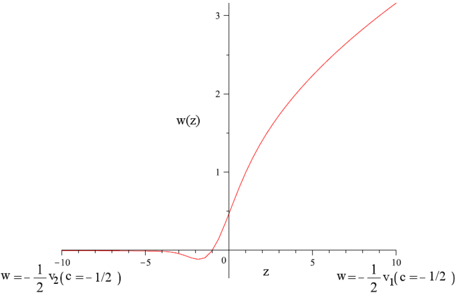
The solutions for various $k$ for $z>0$ can be numerically and analytically shown to match onto the solution for $z<0$, providing a unique[6, 7, 8] non–perturbative completion of the theory. (See figure (1) for an example of a solution found using numerical methods.)

In the $\mu\rightarrow+\infty$ regime, $\Gamma$ represents[8, 11] the number of background ZZ D–branes [29] in the model, while in the $\mu\rightarrow-\infty$ regime, $\Gamma$ represents the number of units of R–R flux in the background[11].

Type 0B string theory coupled to the $(2,4k)$ superconformal minimal models [11] is described by the following string equations[9, 10]:

$\displaystyle\sum_{l=0}^{\infty}t_{l}(l+1)R_{l}=0\ ,\qquad\sum_{l=0}^{\infty}t_{l}(l+1)H_{l}+\nu q=0\ ,$

(9)

where the $R_{l}$ and $H_{l}$ are polynomials of functions $r(x)$ and $\omega(x)$ (and their derivatives), and $\nu$ and $q$ are real constants.

The function ${\widetilde{w}}(x)={r^{2}}/{4}$ defines the partition function of the theory $via$

$${\widetilde{w}}(x)=\frac{r^{2}}{4}=\nu^{2}\frac{d^{2}F}{dx^{2}}\Big|_{\mu=x}\quad.$$

(10)

where $\mu$ is the coefficient of the lowest dimension operator in the world–sheet theory. The $n$th model is chosen by setting all $t_{l}$ to zero except $t_{0}\sim x$ and $t_{n}$. These models have an interpretation as type 0B strings coupled to the $(2,2n)$ superconformal minimal models only for even $n=2k$. The flows between various models are captured by the integrable Zakharov–Shabat (ZS) hierarchy[30].

The asymptotic expansions of the string equations (9) for the first two even $n=2k$ are:

In the $\mu\rightarrow-\infty$ regime, $q$ represents the number of background ZZ D–branes in the model, while in the $\mu\rightarrow\infty$ regime it counts the number of units of R–R flux in the background[11]. The structure of solutions with increasing $n$ is particularly rich [11]; the $n=4$ expansion for $\mu\rightarrow-\infty$ shown above breaks a $\IZ_{2}$ symmetry due to the presence of R–R fields in the dual string theory.

Unlike the 0A case, the solutions for $x>0$ have not been shown numerically to match onto those for $x<0$ so far. The highly non-linear nature of the string equations makes it difficult to numerically obtain smooth solutions connecting the two regimes for the 0B case. Nevertheless, as argued in ref. [11] and reviewed in section 4, these theories can be argued to be non-perturbatively complete in a particular (’t Hooft) limit.

For the $n=2$ ($k=1$) model³³ 3 The central charge of the $\mathcal{N}=1$ $(p,q)$ super–conformal minimal models is given by $\hat{c}=1-\frac{2(p-q)^{2}}{pq}$. For $n=2$, the central charge of the $(2,4)$ superconformal minimal model is thus zero and we simply have the pure world–sheet supergravity sector., the full non–perturbative solution is known since it can be mapped directly to the solution known for the $k=1$ type 0A case $via$ the Morris map [4, 31]. The string equation for the 0A theory becomes the string equation for the 0B theory once one identifies $\Gamma$ with $q$, but with the sign of $x$ reversed. Analogues of the Morris map for higher $n$ are not known.

It is interesting to work out the ’t Hooft limit of the type 0A theories (with string equations (1)). Since, as already discussed, solutions of the full equations have been obtained numerically, it is instructive to compare the ’t Hooft limit (i.e., algebraic) results to the numerical results. (Note that while the last section’s type 0B results were a review, the type 0A analysis is presented here for the first time.)

A modification of the above limit (one that does not affect the physics) will allow us to apply it to the Painlevé IV hierarchy of string equations. The need for such a modification will be explained in the next section.

Instead of rescaling variables in the 0B (0A) theory to eliminate $q$ ($\Gamma$), one can remove the derivatives by first rescaling

$$q\rightarrow\frac{q}{\nu}\quad,$$

(36)

and then taking the limit

$$\nu\rightarrow 0\quad,$$

(37)

in that order, without affecting the physics. Note that the rescaled $q$ is large, so this is still a large $q$ limit. The limit $\nu\rightarrow 0$ amounts to taking $g_{s}\rightarrow 0$, as is clear from the definition of $g_{s}$ ($g_{s}=\frac{\nu}{\mu^{3/2}}$ for $n=2$ and $g_{s}=\frac{\nu}{\mu^{5/4}}$ for $n=4$). This modified limit therefore extracts the physics same as the ’t Hooft limit of the previous subsections.

In this modified limit, the following equations are obtained for the type 0B theories for $n=2$,

$$r^{6}-xr^{4}=2q^{2}\quad,$$

(38)

and for $n=4$,

	$\displaystyle\frac{3}{8}r^{5}-3r^{3}\omega^{2}+r\omega^{4}-\frac{3}{8}xr$	$\displaystyle=$	$\displaystyle 0,$
	$\displaystyle\frac{3}{2}r^{4}\omega-2r^{2}\omega^{3}$	$\displaystyle=$	$\displaystyle-q\quad.$		(39)

These are the same as equations (23) and (27) with $r^{2}\sim f$, $\omega\sim h$ and $x\sim t$, but with the rescaled parameter $q$ explicitly present.

For the 0A theory, after rescaling $\Gamma\rightarrow\frac{\Gamma}{\nu}$, the following equations are obtained for $k=1$ and $k=2$, respectively,

$$w(w-z)^{2}=\Gamma^{2},\qquad w(w^{2}-z)^{2}=\Gamma^{2}\quad.$$

(40)

In fact, for general $k$, the type 0A string equation (1) effectively reduces to

$$w\widetilde{\cal{R}}^{2}=\Gamma^{2}\quad,$$

(41)

where $\widetilde{\cal{R}}=w^{k}-z$ is obtained from $\cal{R}$ after dropping all the derivatives of $w(z)$.

The string equations of the DWW hierarchy (reviewed in section 3) are quite general, encoding the string equations of type 0A and of type 0B as special cases. This generality, however, comes at a price: all but the simplest cases are too complicated to be solved using standard numerical methods. This complicates our task of performing a non–perturbative analysis of the string theories proposed in ref. [20], which were based on strictly perturbative considerations. To facilitate this analysis, we examine the DWW string equations in a (modified) ’t Hooft limit. The result of this study is considerable evidence that the conjectured type II theories possess smooth solutions connecting the perturbative expansions. This analysis also uncovers new non-perturbative solutions, absent from the earlier perturbative analysis, which we suspect may encode new unidentified string theories.

In section 4 we described how to take the ’t Hooft limit of the type 0A and type 0B theories. Implicit in these methods was the fact that the type 0 theories each depend on a single parameter, which counts branes or fluxes. The full DWW equations, in contrast, have two free parameters, so it is not immediately clear how to implement the ’t Hooft limit in this more general case.

The perturbative analysis of ref. [20] suggests that, in addition to the type 0 theories, the full DWW string equations also describe type II theories whose branes and fluxes are counted by a single parameter. This motivates our assumption that new theories are described by a one–dimensional subspace of the parameters $c$ and $\Gamma$. We further restrict our study to subspaces defined by linear combinations of $c$ and $\Gamma$. This is the simplest possibility and although there could be interesting one-dimensional subspaces corresponding to non-trivial curves in $(c,\Gamma)$ parameter space, we will not consider them here.

Given this assumption and the scaling prescription described in section 4.3, we can utilize the ’t Hooft limit to analyze the string equations (13) and (14). For given $\eta$ and $\xi$, let $c+\eta\Gamma=\xi$ be the constraint defining the one-dimensional parameter subspace of a new theory under consideration. Since the constraint is (by assumption) satisfied by the solutions of interest, we can impose the constraint on the DWW equations themselves. We are left with a single free parameter which we can recale as in section 4.3 to take the ’t Hooft limit. In this way we obtain algebraic equations which are simple to analyze.

Unfortunately, in the search for new theories, we do not a priori know the values of $\eta$ and $\xi$, so the above method is not directly applicable. Nevertheless, we can proceed by adopting a slightly different perspective. Note that the constraint $c+\eta\Gamma=\xi$ implies that the free parameter can be taken to be $c$ or $\Gamma$, or any linear combination of them (as long as it is independent of the constraint). Rescaling the free parameter by $1/\nu$ is therefore equivalent to rescaling $c\rightarrow c/\nu$ and $\Gamma\rightarrow\Gamma/\nu$. This procedure is independent of the details of the original constraint, so it can be implemented without actually knowing the values of $\eta$ and $\xi$. The result is a set of algebraic equations which depends on $c$ and $\Gamma$.

Moreover, the solutions to these equations can be used to deduce information about the original constraint. To see this, note that since $\xi$ is a constant, after taking the limit the constraint takes the form $c+\eta\Gamma=0$. Therefore, the original constraint is satisfied by any solution of the algebraic equations which satisfies $c+\eta\Gamma=0$. Turning this around, if a particular solution to the algebraic equations only exists when $c+\eta\Gamma=0$, then this is a strong indication that it descends from the special solution to the full equations subject to $c+\eta\Gamma=\xi$. That is to say, it is an algebraic approximation to the full solutions of some new string theory. Note that $\xi$ is not determined from this approach, but $\eta$ is.

To obtain the algebraic equations, we begin with the DWW string equations (13) and (14),

	$\displaystyle-\frac{1}{2}\mathcal{L}_{x}+\frac{1}{2}u\mathcal{L}+\mathcal{K}$	$\displaystyle=$	$\displaystyle\nu c\quad\quad\quad\quad\quad$
	$\displaystyle\left(-v+\frac{1}{4}u^{2}+\frac{1}{2}u_{x}\right)\mathcal{L}^{2}-\frac{1}{2}\mathcal{L}\mathcal{L}_{xx}+\frac{1}{4}\mathcal{L}_{x}^{2}$	$\displaystyle=$	$\displaystyle\nu^{2}\Gamma^{2}\quad.\quad\quad\quad\quad\quad$

In the modified ’t Hooft limit discussed above,

$\displaystyle\Gamma\rightarrow\frac{\Gamma}{\nu}\quad,\quad c\rightarrow\frac{c}{\nu}\quad,\quad\nu\rightarrow 0\quad,$

(42)

the string equations simplify to

$\displaystyle\frac{1}{2}u\tilde{\mathcal{L}}+\tilde{\mathcal{K}}=c\ ,\qquad{\rm and}\qquad\left(-v+\frac{1}{4}u^{2}\right)\tilde{\mathcal{L}}^{2}=\Gamma^{2}\ ,$

(43)

where $\tilde{\cal{L}}$ and $\tilde{\cal{K}}$ are the polynomials in $u$ and $v$ obtained from $\cal{L}$ and $\cal{K}$ after dropping all the derivative terms. Before analyzing these equations in full generality, let us discuss a few special cases to illustrate our methods.

1. 1.

   $u=0$ (type 0A)
   The restriction to type 0A requires $n$ to be even, in which case $\widetilde{\cal{K}}\propto u$. Thus, setting $u=0$ in first equation of (43) implies $c=0$. This constraint can be written as $c+\eta\Gamma=0$ with $\eta=0$. As described above, this constraint lifts to $c+\eta\Gamma=c=\xi$ at the level of the full equations. If we hadn’t known the parameter constraint of the 0A theory ($c=-\frac{1}{2}$), the algebraic equations alone would indicate that $c=\xi$, a constant.

   Alternatively one could start by looking for solutions to the equations (43) with $c=0$. A subset of smooth solutions, identified by their boundary behavior, will correspond to asymptotic expansions in Classes 1 and 2 with $c$ fixed (recall that these correspond to 0A). The boundary behavior of the smooth solutions is matched with the behavior of expansions in Classes 1 and 2, which are the asymptotic expansions of the type 0A theory.

2. 2.

   $\widetilde{\cal{L}}=0$ (type 0B)
   Setting $\widetilde{\cal{L}}=0$ forces $\Gamma=0$ and the first equation gives $\widetilde{\cal{K}}=c$. For even $n$, these reduce to the 0B algebraic equations after redefining the variables appropriately. The constraint $\Gamma=0$ can be rewritten as $c+\eta\Gamma=0$ with $\eta=\infty$ and lifts to a constraint on the full equations which takes the form $\Gamma=\xi$, a constant. The true parameter constraint for the full $0B$ theory is $\Gamma=0$; the algebraic equations alone do not determine the precise value of $\xi$.

   As in the 0A case above, one could look for smooth solutions to the algebraic equations subject to $\Gamma=0$. If they obey the correct boundary conditions (expansion Classes 1 and 3 (or 5)) one could identify these as 0B solutions.

Our strategy to demonstrate the existence of smooth non–perturbative solutions to the type 0 and type II theories and identify potentially new theories can be summarized as follows. Take the limit (42) of the full DWW equations to obtain a set of algebraic equations. Search for solutions to these equations subject to one of three constraints¹¹¹¹ 11 It turns out that more general linear combinations are relevant only for $n\geq 4$, and for simplicity we exclude such cases from the present analysis.:

$$c=0\ ,\quad\Gamma=0\ ,\quad{\rm or}\quad c\pm\Gamma=0\ .$$

(44)

By matching the asymptotic behavior of these solutions onto the various expansions, we identify the type 0 and type II string theories. We also find new solutions with asymptotics different from those of the type 0 or type II theories. We speculate that these solutions correspond to some new unknown string theories. As emphasized above, the precise parameter constraints of these new theories cannot be fully determined from the algebraic equations.

The string equations for $n=2$ reduce in the algebraic limit (42) to

	$\displaystyle u\left(v+\frac{1}{2}u^{2}+x\right)+2uv$	$\displaystyle=$	$\displaystyle 2c\quad,$
	$\displaystyle\left(uv-c\right)^{2}-v\left(v+\frac{1}{2}u^{2}+x\right)^{2}$	$\displaystyle=$	$\displaystyle\Gamma^{2}\quad.$		(45)

They produce a total of nine asymptotic expansions which fall into 4 classes (see Appendix A). As the expansions within each class are related by various $\mathbb{Z}_{2}$ symmetries [20], we label each expansion only by a subscript specifying its class. The solutions corresponding to the three constraints in parameter space are described below.

1. 1.

   $c=0$
   A plot of solutions to the algebraic equations (45) with $c=0$ and $\Gamma=2$ is shown in figure (7). The plot on the right shows two smooth solutions that connect regions¹²¹² 12 The algebraic solutions are represented by the solid black curves, while the asymptotic expansions are represented by the dashed curves. We adopt this convention in the rest of the paper. of large $-x$ and $+x$. In our conventions, these are $v_{2}|v_{1}$ and $v_{3}|v_{4}$ solutions¹³¹³ 13 We label a solution with $-x$ asymptotics $v_{L}$ and $+x$ asymptotics $v_{R}$ by $v_{L}|v_{R}$.. The plot on the left shows the solutions which do not join negative asymptotics to positive asymptotics, a feature we expect to find in any solutions describing new string theories. For this reason, these types of solutions will not be our primary interest.

   The $v_{2}|v_{1}$ solutions correspond to the 0A theory (with $k=1$) coupled to pure supergravity. It is unclear if the $v_{3}|v_{4}$ solutions correspond to a consistent new theory. Based on the square of theories in figure (2), it is tempting to conclude that this theory might be the type IIA string theory coupled to the $(4,2)$ $(A,D)$ superconformal minimal model. However, as mentioned in the discussion below figure (2), the $v_{4}$ expansion is complex as a $+x$ expansion for $n=2\mod 4$. For the particular case of $n=2$ and $c=0$, $v_{4}$ happens to be real, but this is an exception. We find it unlikely that the corresponding solution to the full equations exists and encodes a consistent theory, but we leave this question for future investigation.

2. 2.

   $\Gamma=0$
   Figure (8) shows the algebraic solutions for $\Gamma=0$ and $c=1.5$. The right figure shows two smooth solutions, $v_{3}|v_{1}$ and $v_{4}|v_{2}$, connecting the negative and positive regions.

   The $v_{3}|v_{1}$ solutions are algebraic approximations to the full solutions of the 0B theory (with $n=2$) coupled to pure supergravity. Analogous to the previous case with $c=0$, it is unclear if the $v_{4}|v_{2}$ solutions descend from a consistent new theory. It is tempting to conclude that these are type IIB string theories coupled to the $(4,2)$ $(A,D)$ superminimal model, but this is likely incorrect because $v_{4}$ is complex as a $+x$ expansion for $n=2\mod 4$.

3. 3.

   $c=\pm\Gamma$
   We consider $c=\Gamma$. The case of $c=-\Gamma$ is completely analogous. Figure (9) shows solutions for $c=2$ and $\Gamma=2$. The solutions in the right figure are $v_{4}|v_{1}$ and $v_{3}|v_{1}$ and connect the negative region smoothly to the positive region.

   The fixed value of $c\mp\Gamma$ cannot be deduced from the algebraic solutions.

References

- [1] C. M. Hull and P. K. Townsend, “Unity of superstring dualities,” Nucl. Phys. B438 (1995) 109–137, arXiv:hep-th/9410167.
- [2] P. K. Townsend, “The eleven-dimensional supermembrane revisited,” Phys. Lett. B350 (1995) 184–187, arXiv:hep-th/9501068.
- [3] E. Witten, “String theory dynamics in various dimensions,” Nucl. Phys. B443 (1995) 85–126, arXiv:hep-th/9503124.
- [4] T. R. Morris, “2-D quantum gravity, multicritical matter and complex matrices,”. FERMILAB-PUB-90-136-T.
- [5] S. Dalley, C. V. Johnson, and T. R. Morris, “Multicritical complex matrix models and nonperturbative 2- D quantum gravity,” Nucl. Phys. B368 (1992) 625–654.
- [6] S. Dalley, C. V. Johnson, and T. R. Morris, “Nonperturbative two-dimensional quantum gravity,” Nucl. Phys. B368 (1992) 655–670.
- [7] C. V. Johnson, T. R. Morris, and A. Watterstam, “Global KdV flows and stable 2-D quantum gravity,” Phys. Lett. B291 (1992) 11–18, arXiv:hep-th/9205056.
- [8] S. Dalley, C. V. Johnson, T. R. Morris, and A. Watterstam, “Unitary matrix models and 2-D quantum gravity,” Mod. Phys. Lett. A7 (1992) 2753–2762, arXiv:hep-th/9206060.
- [9] C. Crnkovic, M. R. Douglas, and G. W. Moore, “Physical solutions for unitary matrix models,” Nucl. Phys. B360 (1991) 507–523.
- [10] T. J. Hollowood, L. Miramontes, A. Pasquinucci, and C. Nappi, “Hermitian vs. Anti-Hermitian 1-matrix models and their hierarchies,” Nucl. Phys. B373 (1992) 247–280, arXiv:hep-th/9109046.
- [11] I. R. Klebanov, J. M. Maldacena, and N. Seiberg, “Unitary and complex matrix models as 1-d type 0 strings,” Commun. Math. Phys. 252 (2004) 275–323, arXiv:hep-th/0309168.
- [12] D. J. Gross and A. A. Migdal, “Nonperturbative Two-Dimensional Quantum Gravity,” Phys. Rev. Lett. 64 (1990) 127.
- [13] E. Brezin and V. A. Kazakov, “Exactly solvable field theories of closed strings,” Phys. Lett. B236 (1990) 144–150.
- [14] M. R. Douglas and S. H. Shenker, “Strings in less than one-dimension,” Nucl. Phys. B335 (1990) 635.
- [15] J. E. Carlisle, C. V. Johnson, and J. S. Pennington, “Baecklund transformations, D-branes, and fluxes in minimal type 0 strings,” J. Phys. A40 (2007) 12451–12462, arXiv:hep-th/0501006.
- [16] J. E. Carlisle, C. V. Johnson, and J. S. Pennington, “D-branes and fluxes in supersymmetric quantum mechanics,” arXiv:hep-th/0511002.
- [17] J. M. Maldacena, “The large N limit of superconformal field theories and supergravity,” Adv. Theor. Math. Phys. 2 (1998) 231–252, arXiv:hep-th/9711200.
- [18] S. S. Gubser, I. R. Klebanov, and A. M. Polyakov, “Gauge theory correlators from non-critical string theory,” Phys. Lett. B428 (1998) 105–114, arXiv:hep-th/9802109.
- [19] E. Witten, “Anti-de Sitter space and holography,” Adv. Theor. Math. Phys. 2 (1998) 253–291, arXiv:hep-th/9802150.
- [20] R. Iyer, C. V. Johnson, and J. S. Pennington, “String Theory and Water Waves,” arXiv:1002.1120 [hep-th].
- [21] D. Kaup, “Finding eigenvalue problems for solving nonlinear evolution equations,” Prog. Theor. Phys. 54 (1975) 72–78.
- [22] D. Kaup, “A higher-order water-wave equation and the method for solving it,” Prog. Theor. Phys. 54 (1975) 396–408.
- [23] L. Broer, “Approximate equations for long water waves,” Appl. Sci. Res. 31 (1975) 377–395.
- [24] B. Kuperschmidt, “Mathematics of dispersive water waves,” Comm. Math. Phys. 99 (1985) 51–73.
- [25] P. R. Gordoa, N. Joshi, and A. Pickering, “On a generalized dispersive water wave hierarchy,” Publ. Res. Inst. Math. Sci. 37 (2001) no. 3, 327–347.
- [26] I. M. Gelfand and L. A. Dikii, “Asymptotic behavior of the resolvent of Sturm-Liouville equations and the algebra of the Korteweg-De Vries equations,” Russ. Math. Surveys 30 (1975) 77–113.
- [27] M. R. Douglas, “Strings in less than one dimension and the generalized KdV hierarchies,” Phys. Lett. B238 (1990) 176.
- [28] T. Banks, M. R. Douglas, N. Seiberg, and S. H. Shenker, “Microscopic and macroscopic loops in non-perturbative two- dimensional gravity,” Phys. Lett. B238 (1990) 279.
- [29] A. B. Zamolodchikov and A. B. Zamolodchikov, “Liouville field theory on a pseudosphere,” arXiv:hep-th/0101152.
- [30] V. E. Zakharov and A. B. Shabat, “Integration of nonlinear equations of mathematical physics by the method of inverse scattering. II,” Funct. Anal. Appl. 13 (1979) 166–174.
- [31] T. R. Morris, “Multicritical matter from complex matrices,” Class. Quant. Grav. 9 (1992) 1873–1881.
- [32] C. V. Johnson, “String theory without branes,” arXiv:hep-th/0610223.