1Introduction

SFB/CPP-10-122

TTP10-48

MZ-TH/10-44

November 2010

$\bar{B}_{s}\rightarrow\phi\rho^{0}$ and $\bar{B}_{s}\rightarrow\phi\pi^{0}$ as a handle on
isospin-violating New Physics

Lars Hofer^a,b, Dominik Scherer^a and Leonardo Vernazza^c^*^* * Alexander-von-Humboldt Fellow

^a Institut für Theoretische Teilchenphysik,
Karlsruhe Institute of Technology, D–76128 Karlsruhe, Germany
^b Institut für Theoretische Physik und Astrophysik,
Universität Würzburg, D–97074 Würzburg, Germany
^c Institut für Physik (THEP),
Johannes Gutenberg-Universität, D–55099 Mainz, Germany

The $2.5\sigma$ discrepancy between theory and experiment observed in the difference $A_{\rm CP}(B^{-}\to\pi^{0}K^{-})-A_{\rm CP}(\bar{B}^{0}\to\pi^{+}K^{-})$ can be explained by a new electroweak penguin amplitude. Motivated by this result, we analyse the purely isospin-violating decays $\bar{B}_{s}\to\phi\rho^{0}$ and $\bar{B}_{s}\to\phi\pi^{0}$ , which are dominated by electroweak penguins, and show that in presence of a new electroweak penguin amplitude their branching ratio can be enhanced by up to an order of magnitude, without violating any constraints from other hadronic $B$ decays. This makes them very interesting modes for LHCb and future $B$ factories. We perform both a model-independent analysis and a study within realistic New Physics models such as a modified- $Z^{0}$ -penguin scenario, a model with an additional $Z^{\prime}$ boson and the MSSM. In the latter cases the new amplitude can be correlated with other flavour phenomena, such as semileptonic $B$ decays and $B_{s}$ - $\bar{B}_{s}$ mixing, which impose stringent constraints on the enhancement of the two $B_{s}$ decays. In particular we find that, contrary to claims in the literature, electroweak penguins in the MSSM can reduce the discrepancy in the $B\to\pi K$ modes only marginally. As byproducts we update the SM predictions to ${\rm Br}(\bar{B}_{s}\to\phi\pi^{0})=1.6^{+1.1}_{-0.3}\cdot 10^{-7}$ and ${\rm Br}(\bar{B}_{s}\to\phi\rho^{0})=4.4^{+2.7}_{-0.7}\cdot 10^{-7}$ and perform a state-of-the-art analysis of $B\rightarrow\pi K$ amplitudes in QCD factorisation.

1 Introduction

At present flavour physics has entered a new exciting era. The new experiment LHCb and the planned super-B-factories will bring the precision of Standard Model (SM) tests and the scope of searches for New Physics (NP) to unseen heights. Particularly important thereby are flavour-changing neutral current (FCNC) decays, which in the SM are highly-suppressed electroweak loop processes. In this work we present a phenomenological analysis of two hadronic FCNC decays, namely $\bar{B}_{s}\rightarrow\phi\rho^{0}$ and $\bar{B}_{s}\rightarrow\phi\pi^{0}$ . We argue that within the next years these decays will become very interesting objects for experimental analyses of the electroweak penguin sector. Up to now, this sector has been tested in hadronic decays only in $B\to\pi K$ modes, and the discrepancies found between the SM prediction and experimental measurements is the main motivation for our work.

The four $B\to\pi K$ decay channels, first observed by the CLEO experiment in the late 1990s [1, 2], have become by now a classic in flavour physics thanks to the precise measurements by BABAR and BELLE. This is also reflected in the large number of theoretical studies of these decays in the SM and various extensions of it. Charged and neutral $B$ mesons can decay to a $\pi K$ final state due to a weak process at the partonic level, $b\rightarrow s\bar{q}q$ with $q=u,d$ . This process is dominated by an FCNC loop governed by the CKM factor $V_{ts}^{*}V_{tb}$ and receives, in the $q=u$ case, also a small tree-level contribution involving the smaller CKM factor $V_{us}^{*}V_{ub}$ . The $B\to\pi K$ branching fractions are therefore small, of order $\mathcal{O}(10^{-6})$ , and sensitive to new FCNCs arising in extensions of the SM. For this reason they are, together with the corresponding CP asymmetries, important observables for tests of the SM flavour structure and for NP searches.

With the data of the $B$ factories having become more and more precise, some discrepancies between $B\to\pi K$ measurements and SM predictions have occurred, provoking speculations on a “ $B\to\pi K$ puzzle”. To date, the measurements of the branching fractions have fluctuated towards the SM predictions, the latter still suffering from large hadronic uncertainties, and only the CP asymmetries show an unexpected behavior [3, 4, 5] manifesting itself in the quantity

\Delta A_{\rm CP}\equiv A_{\rm CP}(B^{-}\to\pi^{0}K^{-})-A_{\rm CP}(\bar{B}^{0}\to\pi^{+}K^{-}).

(1)

For this observable we find in the framework of QCD factorisation (QCDF)

\Delta A_{\rm CP}\stackrel{{\scriptstyle\text{SM}}}{{=}}1.9^{+5.8}_{-4.8}\,\%

(2)

as the SM prediction, which differs significantly from the experimental value

\Delta A_{\rm CP}\stackrel{{\scriptstyle\text{exp.}}}{{=}}(14.8\pm 2.8),\%.

(3)

[6]. Adopting a frequentist approach where we consider a theoretical “error bar” as a range of values definitely containing the true theory result but without assigning any statistical meaning to it [7], this amounts to a $2.5\sigma$ discrepancy.

A point which has received much attention in the literature (see e.g. [8] and references therein) is the fact that the formerly observed discrepancies as well as the currently existing anomaly in $\Delta A_{\rm CP}$ suggest a violation of the strong isospin symmetry beyond the amount expected in the SM. This has often been interpreted as a hint for enhanced electroweak penguins (EW penguins) [9, 10, 11]. We will give a brief overview and discuss the current status of this topic in section 2.1. Whether the $2.5\sigma$ discrepancy in $\Delta A_{\rm CP}$ is a hint for NP in EW penguins or a non-perturbative hadronic effect or simply a statistical fluctuation is controversial. The point that we want to make is that, in order to assess this question, it is highly desirable to obtain further information from other hadronic decays which are sensitive to EW penguin contributions. For this reason we study the purely isospin-violating decays $\bar{B}_{s}\rightarrow\phi\rho^{0}$ and $\bar{B}_{s}\rightarrow\phi\pi^{0}$ , which are dominated by EW penguins, extending and updating our analysis presented in ref. [12]. If NP in this sector exists at a level where it can explain the $\Delta A_{\rm CP}$ puzzle, it could be clearly visible in these purely isospin-violating decays. The upcoming new generation of flavour experiments will have the opportunity to detect these modes for the first time and to measure their branching fractions. The aim of our work is to provide a detailed analysis from the theory side, both in the SM and beyond.

Since the decays $\bar{B}_{s}\rightarrow\phi\rho^{0}$ and $\bar{B}_{s}\rightarrow\phi\pi^{0}$ are not related to other decay modes via flavour symmetries, the non-perturbative part of their decay amplitudes has to be determined from first principles. This can be achieved using the framework of QCDF [13, 14, 15, 16, 17]. This method amounts to a calculation of the hadronic matrix elements up to corrections of order $\Lambda_{\text{QCD}}/m_{B}$ , where $\Lambda_{\text{QCD}}\sim\mathcal{O}(200\,\text{MeV})$ is a typical non-perturbative energy scale of strong interactions. We will use this method throughout the paper in all analyses of $B$ decays to light mesons.

The plan of the paper is as follows: In Chapter 2, we discuss the issue of isospin-violation in $B\to\pi K$ decays and the phenomenology of $\bar{B}_{s}\rightarrow\phi\rho^{0}$ and $\bar{B}_{s}\rightarrow\phi\pi^{0}$ . As a byproduct we provide simple formulas which allow for an easy calculation of various observables concerning these decay modes, taking into account NP effects in EW penguins. Chapter 3 contains a detailed quantitative analysis of $\bar{B}_{s}\rightarrow\phi\rho^{0}$ and $\bar{B}_{s}\rightarrow\phi\pi^{0}$ in different scenarios of a model-independent parameterisation of NP in EW penguins. This analysis is performed in light of our present knowledge on EW penguins from other $B$ decays, in particular $B\to\pi K$ . It is complemented in Chapter 4 with studies of particular extensions of the SM which feature enhanced EW penguins. We conclude in Chapter 5. We keep the main body of the paper free of technicalities and refer the reader interested in technical details to the appendices.

2 Isospin-violation in hadronic $B$ decays

2.1 The $B\to\pi K$ modes

The $B\to\pi K$ decays are dominated by the isospin-conserving QCD penguin amplitude. Nevertheless, they receive small contributions from the tree and the EW penguin amplitude, which are isospin-violating. Combining measurements of the four different decay modes $B^{-}\to\pi^{-}\bar{K}^{0}$ , $B^{-}\to\pi^{0}K^{-}$ , $\bar{B}^{0}\to\pi^{+}K^{-}$ and $\bar{B}^{0}\to\pi^{0}\bar{K}^{0}$ , it is possible to construct observables in which the leading contribution from the QCD penguin drops out, so that they are sensitive to isospin violation.

The mesons participating in $B\to\pi K$ decays transform under isospin rotations as

(\bar{B}^{0},-B^{-})_{1/2}\,,\hskip 28.45274pt(\bar{K}^{0},-K^{-})_{1/2}\,,\hskip 28.45274pt(\pi^{+},-\pi^{0},-\pi^{-})_{1}\,.

(4)

Furthermore we can assign isospin to the operators appearing in the effective Hamiltonian

{\cal H}_{\rm eff}=\frac{G_{F}}{\sqrt{2}}\sum_{p=u,c}\lambda_{p}^{(s)}\left(C_{1}Q_{1}^{p}+C_{2}Q_{2}^{p}+\sum_{i=3}^{10}C_{i}Q_{i}+C_{7\gamma}Q_{7\gamma}+C_{8g}Q_{8g}\right)+\mbox{h.c.},

(5)

which mediates the $B\to\pi K$ transitions. Here $\lambda_{p}^{(s)}=V_{pb}V_{ps}^{*}$ represents a product of elements of the quark mixing (CKM) matrix, $Q_{1,2}^{p}$ are the so-called current-current operators, $Q_{3,\ldots,6}$ are QCD penguin operators, $Q_{7\gamma}$ and $Q_{8g}$ represent the electromagnetic and chromomagnetic operators and

	$\displaystyle Q_{7}=(\bar{s}_{\alpha}b_{\alpha})_{V-A}\textstyle{\sum_{q}\frac{3}{2}}e_{q}(\bar{q}_{\beta}q_{\beta})_{V+A},\hskip 22.99988pt$		$\displaystyle Q_{8}$	$\displaystyle=(\bar{s}_{\alpha}b_{\beta})_{V-A}\textstyle{\sum_{q}\frac{3}{2}}e_{q}(\bar{q}_{\beta}q_{\alpha})_{V+A},$		(6)
	$\displaystyle Q_{9}=(\bar{s}_{\alpha}b_{\alpha})_{V-A}\textstyle{\sum_{q}\frac{3}{2}}e_{q}(\bar{q}_{\beta}q_{\beta})_{V-A},\hskip 22.99988pt$		$\displaystyle Q_{10}$	$\displaystyle=(\bar{s}_{\alpha}b_{\beta})_{V-A}\textstyle{\sum_{q}\frac{3}{2}}e_{q}(\bar{q}_{\beta}q_{\alpha})_{V-A},$		(7)

are the EW penguin operators ( $\alpha,\beta$ denote colours). The latter are of great importance for our work. We define the operators as in [15] so that $C_{1}(M_{W})=1$ at leading order. Containing $\bar{u}u$ - and $\bar{d}d$ -bilinears, the operators $Q_{1}$ ,…, $Q_{10}$ can be distributed among

\mathcal{H}_{\textrm{eff}}\,=\,\mathcal{H}_{\textrm{eff}}^{\Delta I=1}\,+\,\mathcal{H}_{\textrm{eff}}^{\Delta I=0}

(8)

according to the decomposition $1/2\otimes 1/2=1\oplus 0$ [18]. Since the QCD penguin operators $Q_{3,\ldots,6}$ involve the isosinglet combination $(\bar{u}u+\bar{d}d)$ , they contribute solely to $\mathcal{H}_{\textrm{eff}}^{\Delta I=0}$ whereas the other operators give contributions to both parts of $\mathcal{H}_{\textrm{eff}}$ . The $B\to\pi K$ decays thus follow the isospin pattern

1/2\,\stackrel{{\scriptstyle\Delta I=1,0}}{{\longrightarrow}}\,1\otimes 1/2\,=\,3/2\oplus 1/2,

(9)

implying that all four decay amplitudes can be decomposed into three independent isospin amplitudes, $\mathcal{A}^{\Delta I=0}_{1/2}$ , $\mathcal{A}^{\Delta I=1}_{1/2}$ and $\mathcal{A}^{\Delta I=1}_{3/2}$ with the lower index denoting the total isospin of the final state.

One finds that $B\to\pi K$ is dominated by the QCD penguin contribution and thus $|\mathcal{A}^{\Delta I=0}_{1/2}|\gg|\mathcal{A}^{\Delta I=1}_{3/2,\,1/2}|$ . To a first approximation, all the decay modes can be described by the amplitude $\mathcal{A}^{\Delta I=0}_{1/2}$ only, dictating the relative size of the branching fractions to be $1:2:1:2$ (in the same order as in tab. 1).

Refer to caption — Figure 1: Diagrams representing the topological parameterisation in eq. (10) for $B^{-}\to\pi^{0}K^{-}$ . First line from left to right: QCD penguin ( $P$ ), colour-allowed EW penguin ( $r_{\textrm{EW}}$ ), colour-suppressed EW penguin ( $r_{\textrm{EW}}^{\textrm{C}}$ ). Second line from left to right: colour-allowed tree ( $r_{\textrm{T}}$ ), colour-suppressed tree ( $r_{\textrm{C}}$ ), EW penguin annihilation ( $r_{\textrm{EW}}^{\textrm{A}}$ ).

The isospin-invariant amplitudes receive contributions from various SM quark diagrams. It is only at the level of these diagrams that the pattern of CP violation can be correctly implemented, i.e. that the amplitudes $\mathcal{A}^{\Delta I=0}_{1/2}$ , $\mathcal{A}^{\Delta I=1}_{3/2,\,1/2}$ can be related to their CP-conjugated counterparts $\overline{\mathcal{A}}^{\Delta I=0}_{1/2}$ , $\overline{\mathcal{A}}^{\Delta I=1}_{3/2,\,1/2}$ . This suggests an alternative parameterisation of the amplitudes in terms of the topologies of the underlying quark-level transitions [19, 20]:

$\displaystyle{\cal A}(B^{-}\to\pi^{-}\bar{K}^{0})$	$\displaystyle\simeq$	$\displaystyle P\left(1-\frac{1}{3}r^{C}_{\rm EW}+\frac{2}{3}r^{\rm A}_{\rm EW}\right),$
$\displaystyle\sqrt{2}\,{\cal A}(B^{-}\to\pi^{0}K^{-})$	$\displaystyle\simeq$	$\displaystyle P\left(1+r_{\rm EW}+\frac{2}{3}r^{C}_{\rm EW}+\frac{2}{3}r^{\rm A}_{\rm EW}-(r_{\rm T}+r_{\rm C})e^{-i\gamma}\right),$
$\displaystyle{\cal A}(\bar{B}^{0}\to\pi^{+}K^{-})$	$\displaystyle\simeq$	$\displaystyle P\left(1+\frac{2}{3}r^{C}_{\rm EW}-\frac{1}{3}r^{\rm A}_{\rm EW}-r_{\rm T}e^{-i\gamma}\right),$
$\displaystyle\sqrt{2}\,{\cal A}(\bar{B}^{0}\to\pi^{0}\bar{K}^{0})$	$\displaystyle\simeq$	$\displaystyle-\,P\left(1-r_{\rm EW}-\frac{1}{3}r^{C}_{\rm EW}-\frac{1}{3}r^{\rm A}_{\rm EW}+r_{\rm C}e^{-i\gamma}\right).$	(10)

This topological parameterisation is illustrated by the corresponding Feynman diagrams for $B^{-}\to\pi^{0}K^{-}$ in fig. 1. In eq. (10) we have factored out the dominant QCD penguin amplitude $P$ and neglected penguin amplitudes suppressed by $|V_{us}^{*}V_{ub}|/|V_{cs}^{*}V_{cb}|$ . The dependence on the weak CKM phase $\gamma$ has been made explicit, while strong phases are contained in the ratios $r_{i}$ which fulfill $|r_{i}|<1$ . These quantities denote corrections from different types of Feynman diagrams: $r_{\textrm{T}}$ and $r_{\textrm{C}}$ stem from colour-allowed and colour-suppressed tree diagrams, $r_{\textrm{EW}}$ and $r_{\textrm{EW}}^{\textrm{C}}$ from colour-allowed and colour-suppressed EW penguins, respectively. Annihilation via QCD penguin diagrams is absorbed into $P$ whereas weak annihilation via EW penguin diagrams is parameterised by $r_{\textrm{EW}}^{\textrm{A}}$ and colour-suppressed tree annihilation is neglected. With our QCDF setup explained in Appendix A and the expressions for the ratios given in Appendix B we obtain

$\displaystyle r_{\textrm{T}}$	$\displaystyle=$	$\displaystyle 0.17^{+0.07}_{-0.06}\,+\,0.03^{+0.03}_{-0.10}\,i\,,$
$\displaystyle r_{\textrm{C}}$	$\displaystyle=$	$\displaystyle 0.07^{+0.04}_{-0.06}\,+\,(-0.01)^{+0.03}_{-0.05}\,i\,,$
$\displaystyle r_{\textrm{EW}}$	$\displaystyle=$	$\displaystyle\,0.13^{+0.05}_{-0.05}\,+\,0.02^{+0.02}_{-0.07}\,i\,,$
$\displaystyle r_{\textrm{EW}}^{\textrm{C}}$	$\displaystyle=$	$\displaystyle 0.04_{-0.03}^{+0.02}\,+\,(-0.01)_{-0.03}^{+0.02}\,i\,,$
$\displaystyle r_{\textrm{EW}}^{\textrm{A}}$	$\displaystyle=$	$\displaystyle 0.007_{-0.010}^{+0.002}\,+\,(-0.004)_{-0.003}^{+0.011}\,i\,.$	(11)

The result displays the typical features of QCDF predictions, namely small strong phases and large uncertainties of colour-suppressed topologies. The smallness of the $r_{i}$ reflects the domination of the isospin-conserving QCD penguin and justifies the expansion of physical observables in the $r_{i}$ . Among the isospin-violating contributions the colour-allowed tree gives the largest corrections followed by the EW penguin which dominates over the colour-suppressed tree. The colour-suppressed EW penguin ratio $r_{\textrm{EW}}^{\textrm{C}}$ and especially the EW penguin annihilation ratio $r_{\textrm{EW}}^{\textrm{A}}$ are quite small and consequently they have been omitted in most analyses of $B\to\pi K$ decays. In particular, the possibility of having NP in the EW penguin annihilation amplitude $r_{\textrm{EW}}^{\textrm{A}}$ has to our knowledge not been considered so far. However, we want to point out that such an approximation is not valid in the analysis of CP asymmetries: non-vanishing direct CP asymmetries are caused by the interference of parts of the decay amplitude with different weak and strong phases. Consequently direct CP asymmetries in $B\to\pi K$ cannot be generated by the QCD penguin amplitude alone and are automatically sensitive to subleading contributions, encoded in the imaginary parts of the $r_{i}$ coefficients. These, in turn, are generated in QCDF either perturbatively at $\mathcal{O}(\alpha_{s})$ or non-perturbatively at $\mathcal{O}(\Lambda_{\textrm{QCD}}/m_{B})$ . At $\mathcal{O}(\alpha_{s})$ the colour-suppression of $r_{\textrm{EW}}^{\textrm{C}}$ is not present anymore and the $\Lambda_{\textrm{QCD}}/m_{B}$ - suppressed $r_{\textrm{EW}}^{\textrm{A}}$ can compete as well. Therefore we keep $r_{\textrm{EW}}^{\textrm{C}}$ and $r_{\textrm{EW}}^{\textrm{A}}$ in our calculation and we will see in later chapters that we can indeed have a large NP contribution in these amplitudes.

Observable	Theory	Experiment
Br $(\bar{B}^{0}\to\pi^{0}\bar{K}^{0})\cdot 10^{6}$	$5.8^{+5.7}_{-3.6}$	$9.5^{+0.5}_{-0.5}$
Br $(\bar{B}^{0}\to\pi^{+}K^{-})\cdot 10^{6}$	$14.0^{+12.1}_{-7.8}$	$19.4^{+0.6}_{-0.6}$
Br $(B^{-}\to\pi^{0}K^{-})\cdot 10^{6}$	$9.6^{+7.3}_{-4.9}$	$12.9^{+0.6}_{-0.6}$
Br $(B^{-}\to\pi^{-}\bar{K}^{0})\cdot 10^{6}$	$15.7^{+13.7}_{-8.9}$	$23.1^{+1.0}_{-1.0}$
$R_{c}^{B}(\pi K)$	$1.22^{+0.17}_{-0.15}$	$1.12^{+0.07}_{-0.07}$
$R_{n}^{B}(\pi K)$	$1.22^{+0.18}_{-0.16}$	$1.02^{+0.06}_{-0.06}$
$R_{c}^{K}(\pi K)$	$1.27^{+0.12}_{-0.11}$	$1.24^{+0.07}_{-0.07}$
$R_{n}^{K}(\pi K)$	$1.27^{+0.13}_{-0.15}$	$1.13^{+0.08}_{-0.07}$
$R_{c}^{\pi}(\pi K)$	$1.04^{+0.10}_{-0.08}$	$1.11^{+0.06}_{-0.06}$
$R_{n}^{\pi}(\pi K)$	$1.55^{+0.38}_{-0.31}$	$1.26^{+0.09}_{-0.09}$
$R(\pi K)$	$1.02^{+0.02}_{-0.02}$	$1.05^{+0.05}_{-0.05}$
$A_{\rm CP}(\bar{B}^{0}\to\pi^{0}\bar{K}^{0})$	$-0.003^{+0.057}_{-0.108}$	$-0.01^{+0.10}_{-0.10}$
$A_{\rm CP}(\bar{B}^{0}\to\pi^{+}K^{-})$	$-0.047^{+0.187}_{-0.047}$	$-0.098^{+0.012}_{-0.011}$
$A_{\rm CP}(B^{-}\to\pi^{0}K^{-})$	$-0.028^{+0.221}_{-0.059}$	$0.050^{+0.025}_{-0.025}$
$A_{\rm CP}(B^{-}\to\pi^{-}\bar{K}^{0})$	$0.003^{+0.012}_{-0.003}$	$0.009^{+0.025}_{-0.025}$
$\Delta A_{\rm CP}=\Delta A_{\rm CP}^{-}$	$0.019^{+0.058}_{-0.048}$	$0.148^{+0.027}_{-0.028}$
$\Delta A_{\rm CP}^{0}$	$0.006^{+0.118}_{-0.057}$	$0.019^{+0.103}_{-0.103}$
$S_{\rm CP}(\bar{B}^{0}\to\pi^{0}\bar{K}^{0})$	$0.80^{+0.06}_{-0.08}$	$0.57^{+0.17}_{-0.17}$

Table 1: Theoretical vs. experimental results for

\bar{B}\to\pi\bar{K}

decays. The experimental data is taken from [6]. The original results can be found in [21, 22, 23, 24, 25, 26, 27, 28, 29, 30, 31, 32, 33, 34, 35].

One can easily see from eqs. (10,11) that the two amplitudes involved in $\Delta A_{\text{CP}}$ differ only by the subdominant contributions $r_{\textrm{C}}$ , $r_{\textrm{EW}}$ and $r_{\textrm{EW}}^{\textrm{A}}$ , all of which are isospin-violating. Turning to the CP asymmetries, one finds in the SM

	$\displaystyle A_{\rm CP}(B^{-}\to\pi^{0}K^{-})$	$\displaystyle\simeq$	$\displaystyle-2\,{\rm Im}\left(r_{\rm T}+r_{\rm C}\right)\sin\gamma,$
	$\displaystyle A_{\rm CP}(\bar{B}^{0}\to\pi^{+}K^{-})$	$\displaystyle\simeq$	$\displaystyle-2\,{\rm Im}(r_{\rm T})\sin\gamma,$		(12)

with terms quadratic in the $r_{i}$ being neglected. Thus the only possible explanation for a large $\Delta A_{\rm CP}$ in the SM seems to be a large imaginary part of $r_{\textrm{C}}$ , i.e. a large absolute value and large strong phase of the colour-suppressed tree amplitude, generated by some hadronic effects at the low scale $\Lambda_{\text{QCD}}$ which can hardly be calculated perturbatively. However, QCDF predicts only a small $\textrm{Im}(r_{\textrm{C}})$ , insufficient to explain the data, even when all the theory uncertainties are included. Therefore one is tempted to conclude that the discrepancy in $\Delta A_{\rm CP}$ is not due to our lack of understanding of strong interactions but due to isospin-violating NP.

For this reason, $\Delta A_{\rm CP}$ has been studied in various NP models in recent publications [5, 36, 37, 38, 39, 40, 41, 42, 43, 44]. The main ingredient of these analyses is usually an enhancement of the EW penguin topologies by effects of virtual heavy particles. Such contributions can be included into the amplitudes (10) by the replacements

r_{\text{EW}}\rightarrow r_{\text{EW}}+\tilde{r}_{\text{EW}}e^{-i\delta},\hskip 28.45274ptr_{\text{EW}}^{\textrm{C}}\rightarrow r_{\text{EW}}^{\rm C}+\tilde{r}_{\text{EW}}^{\rm C}e^{-i\delta},\hskip 28.45274ptr_{\text{EW}}^{\textrm{A}}\rightarrow r_{\text{EW}}^{\rm A}+\tilde{r}_{\text{EW}}^{\rm A}e^{-i\delta},

(13)

where $\delta$ is a new weak phase and $\tilde{r}_{\text{EW}}^{(i)}$ are complex numbers including a strong phase. The CP asymmetries then become

	$\displaystyle A_{\rm CP}(B^{-}\to\pi^{0}K^{-})$	$\displaystyle\simeq$	$\displaystyle-2\,{\rm Im}\left(r_{\rm T}+r_{\rm C}\right)\sin\gamma+2\,{\rm Im}\left(\tilde{r}_{\text{EW}}+\frac{2}{3}\tilde{r}_{\text{EW}}^{\textrm{C}}+\frac{2}{3}\tilde{r}_{\text{EW}}^{\textrm{A}}\right)\sin\delta,$
	$\displaystyle A_{\rm CP}(\bar{B}^{0}\to\pi^{+}K^{-})$	$\displaystyle\simeq$	$\displaystyle-2\,{\rm Im}(r_{\rm T})\sin\gamma+2\,{\rm Im}\left(\frac{2}{3}\tilde{r}_{\textrm{EW}}^{\textrm{C}}-\frac{1}{3}\tilde{r}_{\textrm{EW}}^{\textrm{A}}\right)\sin\delta,$		(14)

such that

\Delta A_{\rm CP}\,\simeq\,-2\,{\rm Im}\left(r_{\rm C}\right)\sin\gamma+2\,{\rm Im}\left(\tilde{r}_{\text{EW}}+\tilde{r}_{\text{EW}}^{\textrm{A}}\right)\sin\delta

(15)

can turn out to be much larger than in the SM. The observed discrepancy can be solved by a $\tilde{r}_{\text{EW}}$ or a $\tilde{r}_{\text{EW}}^{A}$ term comparable in size to the corresponding SM term $r_{\text{EW}}$ .

Apart from $\Delta A_{\rm{CP}}$ one can also construct other observables from the $B\to\pi K$ data which are sensitive to isospin violation, for example certain ratios of branching fractions. Even though tensions with experimental data in these observables raised the formulation of a ” $B\to\pi K$ puzzle” in the first place [8, 9, 11, 45, 46, 47, 48], in the meantime these quantities are in reasonable agreement with the SM predictions. However, they serve as important constraints for NP in EW penguins and we define and discuss them in Appendix B. Note in particular that the quantity $\Delta A_{\text{CP}}^{0}$ defined there, which is the difference of the two remaining CP asymmetries not appearing in $\Delta A_{\textrm{CP}}$ , probes the same combination of ${\rm Im}(\tilde{r}_{\textrm{EW}})$ and ${\rm Im}(\tilde{r}_{\textrm{EW}}^{\textrm{A}})$ as $\Delta A_{\text{CP}}$ . Unfortunately, data on $A_{\rm CP}(B^{-}\to\pi^{-}\bar{K}^{0})$ and especially on $A_{\rm CP}(\bar{B}^{0}\to\pi^{0}\bar{K}^{0})$ are not good enough yet to gain any information from these observables. Experimental results and SM predictions for the $B\to\pi K$ observables are given in tab. 1.

The main problem which makes it difficult to single out a possible NP contribution in $B\to\pi K$ decays is evident from (10): the colour-allowed EW penguin contributions and colour-suppressed tree contributions enter the amplitudes in (10) exclusively in the combination

r_{\textrm{EW}}\,-\,r_{\textrm{C}}\,e^{-i\gamma}.

(16)

This implies that colour-allowed EW penguins and colour-suppressed trees are inextricably linked with each other, reflecting the fact that the topological parameterisation contains some redundancy. Physical effects found in any experiment cannot unambiguously be attributed to one or the other partner of this topology pair. A new EW penguin contribution $\tilde{r}_{\textrm{EW}}e^{-i\delta}$ can be probed only in one of the four physical combinations

	$\displaystyle{\rm Re}(\tilde{r}_{\textrm{EW}})\cos\delta\,-\,{\rm Re}(r_{\textrm{C}})\cos\gamma\,+\,{\rm Re}(r_{\textrm{EW}})\,,$
	$\displaystyle{\rm Im}(\tilde{r}_{\textrm{EW}})\sin\delta\,-\,{\rm Im}(r_{\textrm{C}})\sin\gamma\,,$
	$\displaystyle{\rm Im}(\tilde{r}_{\textrm{EW}})\cos\delta\,-\,{\rm Im}(r_{\textrm{C}})\cos\gamma\,+\,{\rm Im}(r_{\textrm{EW}})\,,$
	$\displaystyle{\rm Re}(\tilde{r}_{\textrm{EW}})\sin\delta\,-\,{\rm Re}(r_{\textrm{C}})\sin\gamma\,.$		(17)

Therefore, probing $\tilde{r}_{\text{EW}}e^{-i\delta}$ is challenged by the large hadronic uncertainties in the QCDF prediction for $r_{\textrm{C}}$ , which can mimic or hide such a NP signal. One possible way to constrain $r_{C}$ is the approximate $SU(3)$ flavour symmetry which relates it to a corresponding $B\to\pi\pi$ topology. Using this symmetry it has been found that current data on $CP$ violation in $\bar{B}^{0}\to\pi^{0}K_{S}$ is also in disagreement with the SM, independently of $\Delta A_{CP}$ , and can be explained by adding $\tilde{r}_{\text{EW}}$ to the amplitude [42].

The perspective of our work is the following: In order to find out whether the $\Delta A_{\rm CP}$ discrepancy really is a manifestation of isospin-violating physics beyond the SM, one should also study other observables on which such a kind of NP could have a large impact and see whether similar effects appear in measurements of these observables. Our proposal in this work is to test the hypothesis of isospin-violating NP by looking at processes which are highly sensitive to it, namely purely isospin-violating $B_{s}$ decays.

2.2 Purely isospin-violating $B_{s}$ decays

EW penguin contributions to hadronic $B$ decays are usually overshadowed by the larger QCD penguins. This problem can be avoided if one succeeds in probing exclusively the $\Delta I=1$ part of the effective Hamiltonian which is orthogonal to the QCD penguin operators. To achieve this for $B\to\pi K$ , we had to single out the $\Delta I=1$ part of the transition in eq. (9) by combining different isospin-related decay modes, for example by considering the observable $\Delta A_{\textrm{CP}}$ . Our proposal now is to consider decays to which QCD penguins do not contribute at all, i.e. pure $\Delta I=1$ decays, where no such procedure is needed.

There are no two-body decays of the $B^{0}$ or $B^{\pm}$ meson with this property. In these cases the final state would have to be a pure $|3/2,\pm 1/2\rangle$ isospin state which cannot be constructed out of two mesons. The $B_{s}$ meson, on the other hand, is an isosinglet and it can decay as

0\,\stackrel{{\scriptstyle\Delta I=1}}{{\longrightarrow}}\,0\otimes 1\,=\,1\,.

(18)

The final state must consist of an isospin triplet, i.e. $\pi^{0}$ or $\rho^{0}$ , and an isosinglet, i.e. a meson with the flavour structure $s\bar{s}$ . In order to avoid complications stemming from $\eta-\eta^{\prime}$ -mixing, we restrict ourselves to the vector-meson $\phi$ which is to a good approximation a pure $s\bar{s}$ state. This leaves us with the two $\Delta I=1$ channels

$\bar{B}_{s}\to\phi\rho^{0}\hskip 22.99988pt\text{and}\hskip 22.99988pt\bar{B}_{s}\to\phi\pi^{0}$ .

So far only an upper limit ${\rm Br}(\bar{B}_{s}\to\phi\rho^{0})\leq 6.17\cdot 10^{-4}$ exists [49] and no detailed theory analysis of $\bar{B}_{s}\to\phi\rho^{0},\phi\pi^{0}$ has been published. Only the SM branching fractions and CP asymmetries have been calculated in general surveys on $B$ decays to light mesons [16, 17]. In addition, $\bar{B}_{s}\to\phi\pi^{0}$ has been suggested as a tool to measure $\gamma$ via the mixing-induced CP asymmetry [50]. Since in the era of LHCb and super B-factories these two processes will become interesting objects for tests of isospin-violation and potential NP we will in the following study their phenomenology in full detail, in the SM and beyond.

In the SM only three basic topologies are present in these decays, depicted in fig. 2:

•

EW penguins
•

CKM- and colour-suppressed tree diagrams
•

Singlet-annihilation diagrams.

Since the flavour-structure of $\pi^{0}$ and $\rho^{0}$ excludes their production via gluon-exchange, annihilation can only contribute if the $\phi$ meson (the flavour singlet) in the final state is produced from gluons and the second meson comes from weak (as depicted in fig. 2) or electromagnetic interactions. Since the $\phi$ is colour-neutral and it is odd under charge-conjugation, at least three gluons are needed, so that the singlet-annihilation amplitude is formally of higher-order in $\alpha_{s}$ and does not appear in QCDF at the next-to-leading order $\mathcal{O}(\alpha_{s}^{1})$ [16]. However, annihilation topologies in general do not factorise and cannot be calculated perturbatively, because the exchanged gluons may be soft. This means that we can, from a theoretical point of view, only rely on the suppression of these contributions by $\Lambda/m_{B}$ , where $\Lambda$ is a non-perturbative scale, and by $1/N_{c}$ . This leads to the expectation that both the tree and the EW penguin amplitudes can receive corrections of $10\%-20\%$ from singlet-annihilation. However, we can also argue from a phenomenological point of view that $\phi$ -production from three gluons is suppressed by the OZI rule [51, 52, 53, 54] and should thus be only a small effect, even though this rule is theoretically not well understood. In short, our reasoning leads us to the conclusion that in order to test NP in $\bar{B}_{s}\to\phi\rho^{0},\phi\pi^{0}$ , we have to look for new effects which are much larger than this intrinsic uncertainty.

In all our calculations of $\bar{B}_{s}\to\phi\rho^{0},\phi\pi^{0}$ we use the full QCDF decay amplitudes, see refs. [16, 17]. However, since these are quite involved, we now quote simple approximative formulas which can be used as building blocks for an easy calculation of various observables such as branching fractions, CP asymmetries and polarisation fractions. Neglecting singlet-annihilation we can parameterise the amplitudes in analogy to eq. (10) as

\sqrt{2}\mathcal{A}(\bar{B}_{s}\to\phi M_{2})\,=\,P_{\rm EW}^{M_{2}}\left(1-r_{\textrm{C}}^{M_{2}}e^{-i\gamma}\right),

(19)

with $M_{2}$ representing a $\pi^{0}$ , a longitudinal $\rho^{0}$ or a $\rho^{0}$ with negative helicity. The positive helicity amplitude can be neglected in the SM because of its $\Lambda_{\textrm{QCD}}^{2}/m_{B}^{2}$ – suppression. We have factored out the EW penguin amplitude $P_{\rm EW}^{M_{2}}$ anticipating its dominance over the colour-suppressed tree represented by the tree-to-penguin ratio $r_{\textrm{C}}^{M_{2}}$ . A new contribution to the $B\to\pi K$ amplitudes of the form (13) would also enter the $\bar{B}_{s}\to\phi\pi^{0},\phi\rho^{0}$ amplitude (19) modifying it as

\sqrt{2}\,A(\bar{B}_{s}\to\phi M_{2})\,=\,P_{\textrm{EW}}^{M_{2}}\,\left(1\,-\,r^{M_{2}}_{\textrm{C}}\,e^{-i\gamma}\,+\,\tilde{r}_{\textrm{EW}}^{M_{2}}\,e^{-i\delta}\right)\,

(20)

where $\tilde{r}_{\textrm{EW}}^{M_{2}}$ contains a strong phase and $\delta$ is the weak phase introduced in (13). If we assume the new contribution to be of the order of the SM EW penguin, as required by a solution of the “ $\Delta A_{\textrm{CP}}$ -puzzle”, we have $|\tilde{r}_{\textrm{EW}}^{M_{2}}|\sim\mathcal{O}(1)$ and expect a large enhancement of the $\bar{B}_{s}\to\phi\pi^{0},\phi\rho^{0}$ branching fractions, up to an order of magnitude. In order to obtain the same effect within the SM one would have to assume an even larger enhancement of the soft non-perturbative physics entering the colour-suppressed tree topology in $r_{\textrm{C}}^{M_{2}}$ .

Choosing a phase convention such that $P^{M_{2}}_{\textrm{EW}}$ is real, we find

P_{\textrm{EW}}^{\pi}\,=\,6.45^{+1.87}_{-0.54}\cdot 10^{-9},\hskip 28.45274ptP_{\textrm{EW}}^{\rho,0}\,=\,9.95^{+2.83}_{-0.79}\cdot 10^{-9},\hskip 28.45274ptP_{\textrm{EW}}^{\rho,-}\,=\,4.27^{+1.34}_{-0.81}\cdot 10^{-9},

(21)

for the isotriplet meson being $\pi^{0}$ , longitudinal $\rho^{0}$ and $\rho^{0}$ with negative helicity, respectively. We further have

$\displaystyle r^{\pi}_{\textrm{C}}$	$\displaystyle=$	$\displaystyle 0.41_{-0.41}^{+0.37}\,-\,0.13_{-0.30}^{+0.30}\,i\,,$
$\displaystyle r^{\rho,0}_{\textrm{C}}$	$\displaystyle=$	$\displaystyle 0.39_{-0.39}^{+0.35}\,-\,0.13_{-0.29}^{+0.28}\,i\,,$
$\displaystyle r^{\rho,-}_{\textrm{C}}$	$\displaystyle=$	$\displaystyle 0.21_{-0.46}^{+0.49}\,+\,0.15_{-0.45}^{+0.45}\,i\,.$	(22)

Inserting these numbers into eq. (19) we obtain a good approximation of the SM amplitudes for the $\bar{B}_{s}$ decays. Replacing $\gamma\rightarrow-\gamma$ in eq. (19) yields the corresponding CP-conjugated amplitudes ( $B_{s}$ decays). Subsequently one can use the formulas in Appendix A.4 to convert the amplitudes into physical observables. In section 3.1 we extend these prescriptions to physics beyond the SM.

One should keep in mind that the numbers above are calculated using state-of-the-art values for the non-perturbative input parameters, summarised in Appendix A.3. They are based on lattice QCD, QCD sum rules and experimental data. Since our knowledge on these parameters is hopefully going to improve in the future it is desirable to have an additional parameterisation of the decay amplitudes where the non-perturbative input can be changed. We find the dominant sources of theory uncertainties to be (ordered by importance)

•

the form factors $A_{0}^{B_{s}\rightarrow\phi}(0)$ and $F_{\pm}^{B_{s}\rightarrow\phi}(0)$ ,
•

the CKM angle $\gamma$ ,
•

the non-factorisable spectator-scattering amplitudes, parameterised by the complex number $X_{H}$ and the first inverse moment $\lambda_{B_{s}}$ of the $B_{s}$ -meson light-cone distribution amplitude.

The remaining uncertainties, stemming from decay constants, Gegenbauer moments, quark masses and CKM parameters, are much less important so we do not need to display them explicitly. Setting the less important theory parameters to their default values we arrive at the following approximate expressions for the quantities in eqs. (21,22):

$\displaystyle P_{\textrm{EW}}^{\pi}$	$\displaystyle\,=\,$	$\displaystyle 17.0\,A_{0}^{B_{s}\rightarrow\phi}(0)\cdot 10^{-9},\hskip 22.99988ptr^{\pi}_{\textrm{C}}$	$\displaystyle\,=\,$	$\displaystyle-0.12i-0.02+\frac{0.01\text{GeV}(1+X_{H})}{A_{0}^{B_{s}\rightarrow\phi}(0)\lambda_{B_{s}}}$
$\displaystyle P_{\textrm{EW}}^{\rho,0}$	$\displaystyle\,=\,$	$\displaystyle 26.2\,A_{0}^{B_{s}\rightarrow\phi}(0)\cdot 10^{-9},\hskip 22.99988ptr^{\rho,0}_{\textrm{C}}$	$\displaystyle\,=\,$	$\displaystyle-0.13i-0.02+\frac{0.01\text{GeV}(1+X_{H})}{A_{0}^{B_{s}\rightarrow\phi}(0)\lambda_{B_{s}}}$
$\displaystyle P_{\textrm{EW}}^{\rho,-}$	$\displaystyle\,=\,$	$\displaystyle 6.6\,F_{-}^{B_{s}\rightarrow\phi}(0)\cdot 10^{-9},\hskip 22.99988ptr^{\rho,-}_{\textrm{C}}$	$\displaystyle\,=\,$	$\displaystyle 0.14i-0.06-\frac{0.02\text{GeV}(1-X_{H})}{F_{-}^{B_{s}\rightarrow\phi}(0)\lambda_{B_{s}}}.$	(23)

The tree topologies $r^{M_{2}}_{\textrm{C}}$ suffer from the large spectator-scattering uncertainties due to a strong cancellation between the leading order and QCD vertex corrections. Again one can insert these formulas into eq. (19), this time with arbitrary values and uncertainties for the form factors and spectator-scattering parameters, and use the definitions in Appendix A.4 to calculate physical observables. CP conjugation again amounts to replacement $\gamma\rightarrow-\gamma$ .

We conclude this section quoting our QCDF results for the SM values of the $\bar{B}_{s}\to\phi\pi^{0},\phi\rho^{0}$ observables. As for the CP-averaged branching fractions we obtain

{\rm Br}(\bar{B}_{s}\to\phi\pi^{0})\,=\,1.6^{+1.1}_{-0.3}\cdot 10^{-7},\hskip 42.67912pt{\rm Br}(\bar{B}_{s}\to\phi\rho^{0})\,=\,4.4^{+2.7}_{-0.7}\cdot 10^{-7}.

(24)

For comparison we also quote the approximate result according to (23):

{\rm Br}(\bar{B}_{s}\to\phi\pi^{0})\,=\,1.6^{+1.0}_{-0.3}\cdot 10^{-7},\hskip 42.67912pt{\rm Br}(\bar{B}_{s}\to\phi\rho^{0})\,=\,4.4^{+2.4}_{-0.7}\cdot 10^{-7}.

(25)

The smallness of the SM branching ratios compared to other hadronic $B$ decays is due to the absence of QCD penguins and non-suppressed tree-level contributions. The measurement of these branching fractions is thus challenging and has not been achieved yet. However, we will show in later chapters that NP in EW penguins has the chance to enhance the BRs by up to an order of magnitude, such that this measurement is a very interesting project. We expect that LHCb will be able to measure ${\rm Br}(\bar{B}_{s}\rightarrow\phi\rho^{0})$ while the $\bar{B}_{s}\rightarrow\phi\pi^{0}$ mode is more suitable for a super B-factory where a full reconstruction can cure the notorious difficulties with the identification of neutral pions. In case of a strong enhancement $\bar{B}_{s}\rightarrow\phi\rho^{0}$ should also be visible in the Tevatron data [55]. The branching ratio ${\rm Br}(\bar{B}_{s}\to\phi\rho^{0})$ is dominated by the longitudinal polarisation state as can be seen in

{\rm Br}(\bar{B}_{s}\to\phi_{L}\rho^{0}_{L})\,=\,3.7^{+2.5}_{-0.7}\cdot 10^{-7}\,

(26)

and the longitudinal polarisation fraction

f_{\textrm{L}}\,=\,0.84^{+0.08}_{-0.11}\,.

(27)

As stated above, one of the main sources of uncertainty in the QCDF predictions is the form factor $A_{0}^{B_{s}\to\phi}$ . It can in principle be eliminated by considering the ratios

\frac{{\rm Br}(\bar{B}_{s}\rightarrow\phi\rho^{0})}{{\rm Br}(\bar{B}_{s}\rightarrow\phi\pi^{0})}=2.83^{+0.35}_{-0.23},\hskip 22.99988pt\hskip 22.99988pt\frac{{\rm Br}(\bar{B}_{s}\rightarrow\phi_{L}\rho^{0}_{L})}{{\rm Br}(\bar{B}_{s}\rightarrow\phi\pi^{0})}=2.38^{+0.10}_{-0.08}\,.

(28)

NP could still be visible in these ratios because in many scenarios it enters $\bar{B}_{s}\rightarrow\phi\rho^{0}$ and $\bar{B}_{s}\rightarrow\phi\pi^{0}$ in different ways. The cancellation of $A_{0}^{B_{s}\to\phi}$ also occurs in the ratios

	$\displaystyle\frac{{\rm Br}(\bar{B}_{s}\rightarrow\phi\pi^{0})}{{\rm Br}(\bar{B}_{s}\rightarrow\phi\phi)}$	$\displaystyle=$	$\displaystyle 0.007^{+0.008}_{-0.004},$
	$\displaystyle\frac{{\rm Br}(\bar{B}_{s}\rightarrow\phi\rho^{0})}{{\rm Br}(\bar{B}_{s}\rightarrow\phi\phi)}$	$\displaystyle=$	$\displaystyle 0.020^{+0.023}_{-0.010},\hskip 11.49994pt\frac{{\rm Br}(\bar{B}_{s}\rightarrow\phi_{L}\rho^{0}_{L})}{{\rm Br}(\bar{B}_{s}\rightarrow\phi\phi)}=0.017^{+0.019}_{-0.009}.$		(29)

There however this gain is compensated by additional uncertainties arising from the QCD-penguin-dominated decay $\bar{B}_{s}\rightarrow\phi\phi$ . The experimental benefit in these last ratios is that at LHCb absolute branching ratios cannot be measured because the absolute number of $B_{s}$ mesons is unknown. Finally, we find the direct CP asymmetries to be very uncertain:

A_{\rm CP}^{\text{dir}}(\bar{B}_{s}\rightarrow\phi\rho^{0})=0.19^{+0.53}_{-0.61},\hskip 22.99988pt\hskip 22.99988ptA_{\rm CP}^{\text{dir}}(\bar{B}_{s}\rightarrow\phi\pi^{0})=0.27^{+0.50}_{-0.62}.

(30)

Due to the smallness of the branching ratios, these CP asymmetries are also difficult to access experimentally, therefore we will not consider them any further.

3 Model-independent analysis

In the previous chapter we proposed to test the hypothesis of NP in the EW penguin sector, as suggested by the discrepancy in the $B\to\pi K$ observable $\Delta A_{\textrm{CP}}$ , by a measurement of the decays $\bar{B}_{s}\to\phi\pi^{0},\phi\rho^{0}$ . In this chapter we support our proposal by a quantitative analysis pursuing the following strategy: We parameterise NP in EW penguins in a model-independent way by adding corresponding terms to the Wilson coefficients $C_{7}^{(\prime)},...,C_{10}^{(\prime)}$ . By performing a $\chi^{2}$ -fit we determine the NP parameters in such a way that they describe well the $B\to\pi K$ data. In particular they should allow for a solution of the $\Delta A_{\textrm{CP}}$ discrepancy. Further hadronic decays like $B\to\rho K,\pi K^{*},\rho K^{*}$ are used to impose additional constraints at the $2\,\sigma$ level. With respect to the resulting fit we study the decays $\bar{B}_{s}\to\phi\pi^{0},\phi\rho^{0}$ and quantify a potential enhancement of their branching fractions. Note that such an exhaustive analysis, correlating different hadronic decay modes with sensitivity to isospin violation, is only possible if hadronic matrix elements are calculated from first principles like in the framework of QCDF. A method based on flavour symmetries, as it has been used in most studies of $B\to\pi K$ decays so far, could not achieve this. In particular, the decays $\bar{B}_{s}\to\phi\pi^{0},\phi\rho^{0}$ , which are our main interest, are not related to any other decay via $SU(3)_{F}$ so their branching fractions cannot be predicted in this way.

3.1 Modified EW penguin coefficients

In the SM the Wilson coefficients $C_{7},...,C_{10}$ obey the hierarchy $|C_{9}|\gg|C_{7}|\gg|C_{8}|,|C_{10}|$ at the electroweak scale. This is because $C_{9}$ receives $1/\sin^{2}\theta_{W}$ -enhanced contributions from $Z$ -penguin and box diagrams in contrast to $C_{7}$ , while $C_{8,10}$ are generated for the first time at two-loop level due to their colour structure. For our model-independent analysis we consider arbitrary NP contributions to the coefficients $C_{7}$ and $C_{9}$ as well as to their mirror counterparts $C_{7}^{\prime}$ and $C_{9}^{\prime}$ . Normalizing the new coefficients to the SM value $C_{9}^{\rm LO}$ defined in eq. (59) in the appendix, we have

C_{7,9}^{(\prime)\rm NP}(M_{W})=C_{9}^{\rm LO}(M_{W})\,q_{7,9}^{(\prime)},\hskip 22.99988pt\hskip 22.99988ptq_{7,9}^{(\prime)}=|q_{7,9}^{(\prime)}|e^{i\phi_{7,9}^{(\prime)}},

(31)

where $\phi_{7,9}^{(\prime)}$ are new weak phases. The coefficient $C_{9}^{\rm LO}$ contains the parts of $C_{9}^{\textrm{SM}}$ enhanced by $m_{t}^{2}/M_{W}^{2}$ and $1/\sin^{2}\theta_{W}$ , as explained in Appendix A.1. There we also describe the scheme which we use for the renormalisation-group evolution. Applying it to the NP coefficients leads to the low-scale values displayed in tab. 2. They can be compared to the dominant SM coefficient $C^{\text{SM}}_{9}(m_{b})/\alpha=-1.203$ .

	$C^{\rm NP}_{i}(m_{b})/\alpha$	$C_{i}^{\rm{NP}\,\prime}(m_{b})/\alpha$
$C_{7}$	$-0.966\,q_{7}+0.009\,q_{9}$	$-0.966\,q_{7}^{\prime}+0.009\,q_{9}^{\prime}$
$C_{8}$	$-0.387\,q_{7}+0.002\,q_{9}$	$-0.387\,q_{7}^{\prime}+0.002\,q_{9}^{\prime}$
$C_{9}$	$0.010\,q_{7}-1.167\,q_{9}$	$0.010\,q_{7}^{\prime}-1.167\,q_{9}^{\prime}$
$C_{10}$	$-0.001\,q_{7}+0.268\,q_{9}$	$-0.001\,q_{7}^{\prime}+0.268\,q_{9}^{\prime}$

Table 2: NLO short-distance coefficients of the EW penguin operators at the scale

m_{b}

. Modifications to other short-distance coefficients are negligible.

In our analysis we will study several different scenarios. First, we consider the cases where only one of the coefficients $q_{7}$ , $q_{9}$ , $q_{7}^{\prime}$ , $q_{9}^{\prime}$ is different from zero. This means we assume the dominance of an individual NP operator as it has also been done for example in ref. [41]. Second, we consider the possibilities of having $q_{7}=q_{9}$ , $q_{7}^{\prime}=q_{9}^{\prime}$ , $q_{7}=q_{9}^{\prime}$ and $q_{7}^{\prime}=q_{9}$ . Finally, we study parity-symmetric new contributions corresponding to the three cases $q_{7}=q_{7}^{\prime}$ , $q_{9}=q_{9}^{\prime}$ and $q_{7}=q_{7}^{\prime}=q_{9}=q_{9}^{\prime}$ . Each of these scenarios can be described by means of two real parameters, the absolute value $|q|$ and phase $\phi$ of the NP contribution under consideration. This reduced number of free parameters allows us to perform a fit to $B\to\pi K$ data and to draw meaningful conclusions on the $\bar{B}_{s}\to\phi\pi^{0},\phi\rho^{0}$ decays. The study of this large set of well-motivated simplified scenarios is assumed to represent all relevant features of the general framework with unrelated $q_{7}$ , $q_{9}$ , $q_{7}^{\prime}$ , $q_{9}^{\prime}$ .

Our main motivation for adding NP to the coefficients $C_{7}^{(\prime)},C_{9}^{(\prime)}$ was the claim that the $\Delta A_{\textrm{CP}}$ discrepancy can be solved in this way, namely by generating the terms $\tilde{r}_{\textrm{EW}}$ , $\tilde{r}_{\textrm{EW}}^{\textrm{C}}$ , $\tilde{r}_{\textrm{EW}}^{\textrm{A}}$ introduced in eq. (13). Introducing individual terms for each of the four relevant Wilson coefficients, we obtain

$\displaystyle\sum\limits_{i=7,9,7^{\prime},9^{\prime}}\tilde{r}_{\textrm{EW},\,i}\,e^{-i\delta_{i}}$	$\displaystyle=$	$\displaystyle(q_{7}-q_{7}^{\prime})\,\left[\,(-0.12)^{+0.04}_{-0.05}\,+\,(-0.02)^{+0.07}_{-0.02}\,i\,\right]\,+$
		$\displaystyle(q_{9}-q_{9}^{\prime})\,\left[\,0.12^{+0.05}_{-0.04}\,+\,0.02^{+0.02}_{-0.07}\,i\,\right]\,,$
$\displaystyle\sum\limits_{i=7,9,7^{\prime},9^{\prime}}\tilde{r}_{\textrm{EW},\,i}^{\textrm{C}}\,e^{-i\delta_{i}}$	$\displaystyle=$	$\displaystyle(q_{7}-q_{7}^{\prime})\,\left[\,0.10^{+0.03}_{-0.02}\,+\,0.01^{+0.01}_{-0.06}\,i\,\right]\,+$
		$\displaystyle(q_{9}-q_{9}^{\prime})\,\left[\,0.04^{+0.02}_{-0.03}\,+\,(-0.005)^{+0.016}_{-0.026}\,i\,\right]\,,$

	$\displaystyle\sum\limits_{i=7,9,7^{\prime},9^{\prime}}\tilde{r}_{\textrm{EW},\,i}^{\textrm{A}}\,e^{-i\delta_{i}}$	$\displaystyle=$	$\displaystyle(q_{7}-q_{7}^{\prime})\,\left[\,0.03^{+0.04}_{-0.07}\,+\,(-0.06)^{+0.12}_{-0.01}\,i\,\right]\,+$		(32)
			$\displaystyle(q_{9}-q_{9}^{\prime})\,\left[\,0.007^{+0.003}_{-0.010}\,+\,(-0.006)^{+0.012}_{-0.003}\,i\,\right]\,.$		(32)

Let us briefly discuss the main characteristics of these coefficients:

•

First of all, note that parity-symmetric models obviously do not contribute to $B\to\pi K$ at all. This general feature of $B$ decays into two pseudoscalar mesons ( $PP$ decays) follows from eq. (74). Therefore such a scenario cannot solve the $\Delta A_{\textrm{CP}}$ discrepancy.
•

The contributions $\tilde{r}_{\textrm{EW},\,7^{(\prime)}}$ and $\tilde{r}_{\textrm{EW},\,9^{(\prime)}}$ tend to cancel each other. Hence in the scenarios with $q_{7}=q_{9}$ and $q_{7}^{\prime}=q_{9}^{\prime}$ only a negligible new colour-allowed EW penguin contribution is generated.
•

Whereas ${\rm Re}(\tilde{r}_{\textrm{EW},\,9^{(\prime)}}^{\textrm{C}})$ features the typical colour-suppression with respect to ${\rm Re}(\tilde{r}_{\textrm{EW},\,9^{(\prime)}})$ , this pattern is not obeyed by the $q_{7}^{(\prime)}$ terms. This is due to a conspirative interplay of the large mixing of $C_{7}^{(\prime)}$ into $C_{8}^{(\prime)}$ (compare tab. 2), constructive interference of the new $C_{7}^{(\prime)}$ and $C_{8}^{(\prime)}$ contributions in the QCDF coefficient $a_{8}^{(\prime)}$ and a chiral enhancement factor $r_{\chi}^{\pi,K}\approx 1.5$ multiplying $a_{8}^{(\prime)}$ in eq. (A.2) for the topological amplitude. None of these three effects is present in the $q_{9}^{(\prime)}$ case.
•

The annihilation coefficient $\tilde{r}_{\textrm{EW},\,7^{(\prime)}}^{\textrm{A}}$ develops a large imaginary part. In scenarios with non-vanishing $q_{7}^{(\prime)}$ this term gives the dominant contribution to $\Delta A_{\textrm{CP}}$ .

From eq. (15) we see that the $\Delta A_{\textrm{CP}}$ discrepancy can be solved either through $\tilde{r}_{\textrm{EW}}$ or through $\tilde{r}_{\textrm{EW}}^{\textrm{A}}$ . Except for the parity-symmetric models, all the scenarios mentioned above can achieve such a solution. In fig. 3 this is illustrated for the cases with a single $q_{7}$ or $q_{9}$ and for the $q_{7}=q_{9}$ scenario. Graphs for the respective mirror scenarios are obtained by a $180^{\circ}$ rotation. The yellow region contains those points of the $({\rm Re}(q_{i}),{\rm Im}(q_{i}))$ - plane for which the theory error band overlaps with the experimental $1\,\sigma$ region, whereas the blue region represents those points for which also the experimental central value lies within the theory error interval. The red circle illustrates the minimal $|q|$ - value needed to reduce the $\Delta A_{\textrm{CP}}$ tension below the $1\,\sigma$ level. For the three scenarios in fig. 3 we read off $|q_{7}|\gtrsim 0.3$ , $|q_{9}|\gtrsim 0.8$ and $|q_{7}|=|q_{9}|\gtrsim 0.4$ . The fact that in the $q_{7}=q_{9}$ case only a small NP contribution is needed, in spite of the absence of $\tilde{r}_{\textrm{EW}}$ , demonstrates the importance of the annihilation term $\tilde{r}_{\textrm{EW}}^{\textrm{A}}$ . Finally, we like to stress that the solution of the $\Delta A_{\textrm{CP}}$ discrepancy via a minimal $|q|$ - value requires the adjustment of the phase $\phi$ to a certain value. Realistic scenarios avoiding such a fine-tuning have larger $|q|$ - values, typically $|q|\sim 1$ .

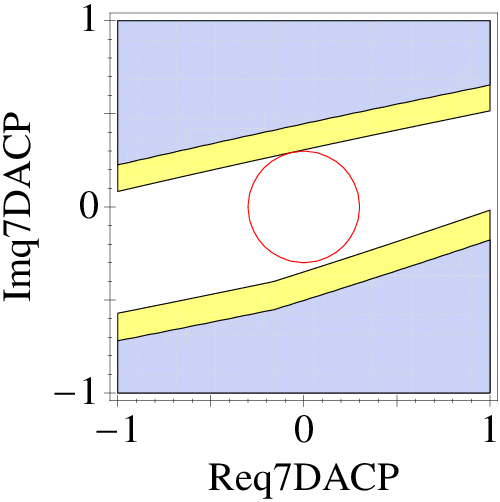
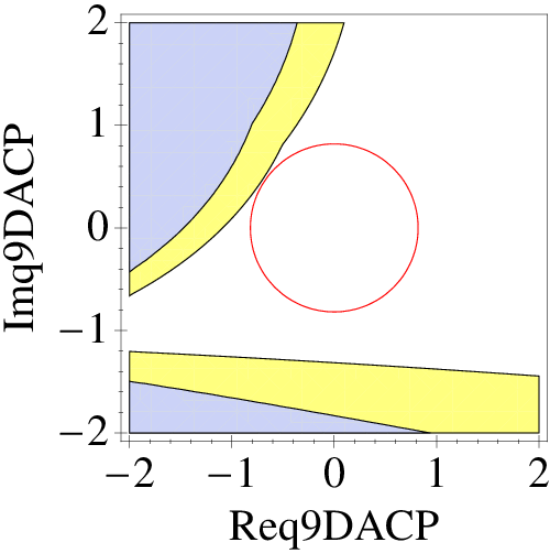
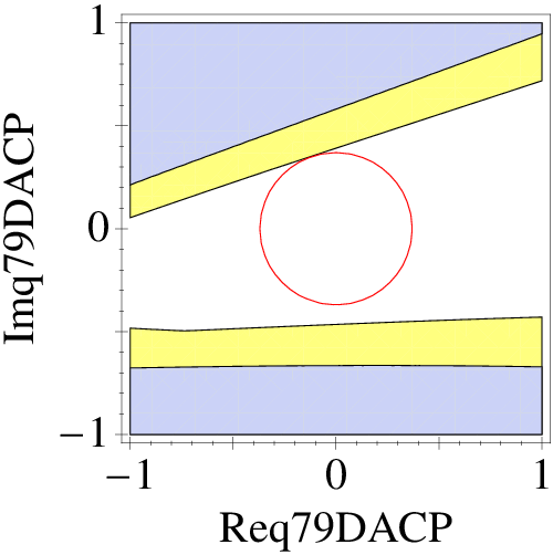
Our main goal is to study the impact of such a NP scenario on the decays $\bar{B}_{s}\to\phi\pi^{0},\phi\rho^{0}$ . The NP contributions to $C_{7}^{(\prime)},...,C_{10}^{(\prime)}$ generate the $\tilde{r}_{\textrm{EW}}^{M_{2}}$ - terms introduced in eq. (20). Introducing again individual terms for contributions from the various Wilson coefficients, they read for the four different amplitudes

$\displaystyle\sum\limits_{i=7,9,7^{\prime},9^{\prime}}\tilde{r}_{\textrm{EW},\,i}^{\pi}\,e^{-i\delta_{i}}$	$\displaystyle=$	$\displaystyle-0.9\,\left(q_{7}\,+\,q_{7}^{\prime}\,-\,q_{9}\,-\,q_{9}^{\prime}\right),$
$\displaystyle\sum\limits_{i=7,9,7^{\prime},9^{\prime}}\tilde{r}_{\textrm{EW},\,i}^{\rho,0}\,e^{-i\delta_{i}}$	$\displaystyle=$	$\displaystyle\phantom{-}0.9\,\left(q_{7}\,-\,q_{7}^{\prime}\,+\,q_{9}\,-\,q_{9}^{\prime}\right),$
$\displaystyle\sum\limits_{i=7,9,7^{\prime},9^{\prime}}\tilde{r}_{\textrm{EW},\,i}^{\rho,-}\,e^{-i\delta_{i}}$	$\displaystyle=$	$\displaystyle-0.6\,\left(q_{7}\,+\,q_{9}\right),$
$\displaystyle\sum\limits_{i=7,9,7^{\prime},9^{\prime}}\tilde{r}_{\textrm{EW},\,i}^{\rho,+}\,e^{-i\delta_{i}}$	$\displaystyle=$	$\displaystyle\phantom{-}0.6\,\left(q_{7}^{\prime}\,+\,q_{9}^{\prime}\right)\times P_{\textrm{EW}}^{\rho,-}/P_{\textrm{EW}}^{\rho,+}\,,$	(33)

where we have neglected $q_{7,9}$ -contributions to $\tilde{r}_{\textrm{EW}}^{\rho,+}$ and $q_{7,9}^{\prime}$ -contributions to $\tilde{r}_{\textrm{EW}}^{\rho,-}$ according to their $\Lambda_{\textrm{QCD}}^{2}/m_{B}^{2}$ suppression. The SM EW penguin amplitude $P_{\textrm{EW}}^{\rho,+}$ drops out of the total expression (20) of the amplitude, $P_{\textrm{EW}}^{\rho,-}$ is given in eq. (21). The parameters $\tilde{r}_{\textrm{EW}}^{M_{2}}$ develop only very small strong phases and uncertainties not indicated in (33). This is because they are ratios of equal topologies such that uncertainties and strong phases approximately cancel.

We have stated the expressions in eq. (33) for two reasons: Firstly we want to show the main consequences of non-vanishing $q_{7,9}^{(\prime)}$ for the $\bar{B}_{s}\to\phi\pi^{0},\phi\rho^{0}$ decays. We see that for $|q_{i}|=\mathcal{O}(1)$ indeed new contributions with the magnitude of the leading SM EW penguin are generated. While parity-symmetric NP was invisible in $B\to\pi K$ , it could be detected in $\bar{B}_{s}\to\phi\pi^{0}$ and in principle also in $\bar{B}_{s}\to\phi\rho^{0}$ due to the different interference patterns of $\tilde{r}_{\textrm{EW}}^{\rho,-}$ and $\tilde{r}_{\textrm{EW}}^{\rho,+}$ with the corresponding SM contributions. Furthermore, left- and right-handed NP could be distinguished by a polarisation measurement of $\bar{B}_{s}\to\phi\rho^{0}$ . This general feature of decays to vector-vector final states has been pointed out by Kagan [56]. Note that the question of left- vs. right-handed NP cannot be answered from $B\to\pi K$ alone since, as we have seen, the two scenarios differ only by a rotation in the NP parameter space.

The second benefit of eq. (33) is that it allows for a simple calculation of $\bar{B}_{s}\to\phi\pi,\phi\rho$ observables to a very good accuracy. In this way it permits a study of these decays without the extensive implementation of QCDF. One simply evaluates the amplitude eq. (20) inserting eqs. (21,22) - or alternatively eq. (23) - and the NP part from eq. (33). The CP-conjugated amplitude is obtained by flipping the sign of $\gamma$ and replacing the $q_{i}$ by their complex conjugates. Subsequently one can use the formulas in Appendix A.4 to calculate observables.

3.2 Fit to $B\to\pi K$ data and constraints from other decays

The four $B\to\pi K$ channels are the most precisely measured hadronic $b\rightarrow s$ decays. For this reason, we use experimental information from these channels as input for our quantitative NP analysis by performing a fit of $q_{7}^{(\prime)}$ and $q_{9}^{(\prime)}$ to $B\to\pi K$ data. This fit will be an indication for values of the $q_{i}^{(\prime)}$ that are realistic to expect and consequently will enable us to find an expected size of enhancement of the branching ratios of $\bar{B}_{s}\to\phi\rho^{0}$ and $\bar{B}_{s}\to\phi\pi^{0}$ . In the treatment of theoretical and experimental uncertainties in the fit we follow the Rfit scheme [7]. More details on this issue are given in Appendix C.

Since $B\to\pi K$ decays are greatly dominated by QCD penguins and since they suffer from large theoretical uncertainties, it is obvious that NP effects residing in EW penguins are difficult to find in branching ratios and direct CP asymmetries. It is more useful to consider instead particular combinations of these basic observables which highlight the isospin-violating contributions and can be predicted with a better precision. For example, it is difficult to see a need for isospin-violating NP by looking at the two CP asymmetries entering in $\Delta A_{\rm CP}$ (see tab. 1) since both of them have more than $100\%$ theoretical uncertainty, reflecting the difficulty of predicting strong phases in QCDF. In the difference $\Delta A_{\rm CP}$ , the theory uncertainties cancel to a large extent such that the discrepancy with experimental data becomes clearer. Moreover, in realistic models a new contribution in the EW penguin sector usually comes in combination with NP of comparable size in the QCD penguins since the new contribution in general matches onto a linear combination of the QCD and EW penguin operators. By considering mainly isospin-violating observables, one reduces the sensitivity to additional effects from new contributions to $C_{3},...,C_{6}$ which we did not include in our parameterisation (31).

For our $B\to\pi K$ fit, we use suitable ratios of branching fractions and differences of CP asymmetries as well as the mixing-induced CP asymmetry in $\bar{B}^{0}\to\pi^{0}\bar{K}^{0}$ as input. The definitions of these quantities are summarised in Appendix B. Many of these quantities have also been considered in the past in the context of flavour symmetry analyses of $B\to\pi K$ decays. A summary of theoretical predictions vs. experimental results for all these observables as well as for the $B\to\pi K$ branching fractions and CP asymmetries is provided in tab. 1. At present none of these quantities deviates from the SM prediction by more than $~1\sigma$ apart from $\Delta A_{\rm CP}$ . We thus expect $\Delta A_{\rm CP}$ (and to a lower degree also $S_{\textrm{CP}}$ ) to pull the fit towards non-zero values of the $q_{i}^{(\prime)}$ whereas the other observables will favour values close to the origin of the complex plane.

In addition to the fit we consider constraints on the NP parameters arising from a large number of hadronic B decays. To this end we compare the theoretical prediction of an observable as a function of the $q_{i}^{(\prime)}$ to its measured value and extract a $2\sigma$ -constraint as follows:

{\rm Point[q_{7,9}^{(\prime)}\,\,space]}=\left\{\begin{array}[]{cl}{\rm allowed}&\mbox{ if }\left\{\begin{array}[]{l}(x_{\rm theo}+\sigma_{\rm theo,\,sup})>(x_{\rm exp}-2\sigma_{\rm exp,\,inf})\\ \textrm{ and }(x_{\rm theo}-\sigma_{\rm theo,\,inf})<(x_{\rm exp}+2\sigma_{\rm exp,\,sup}),\end{array}\right.\\ {\rm excluded}&\mbox{ otherwise}.\\ \end{array}\right.

(34)

Here $(x_{\rm theo})^{+\sigma_{\rm theo,\,sup}}_{-\sigma_{\rm theo,\,inf}}$ represents the theoretical prediction for the respective physical observable. The uncertainty does not imply a particular probability distribution but the true value is supposed to lie within the error interval. For the experimental value $x_{\rm exp}\pm\sigma_{\rm exp}$ a Gaussian error is assumed.

This procedure is applied to data from $B\to\pi K$ as well as to data from the $B\to\rho K$ , $B\to\pi K^{*}$ and $B\to\rho K^{(*)}$ decay channels, which are simply the pseudoscalar-vector ( $PV$ ) and vector-vector ( $VV$ ) modes corresponding to $B\to\pi K$ . The $PV$ and $VV$ modes turn out to be more sensitive to isospin-violating flavour topologies than their $PP$ counterparts because the leading QCD penguin amplitude is smaller. Experimental information on these decays, however, is not (yet) as precise as the available data for the $\pi K$ modes. Therefore we do not include the $PV$ , $VV$ modes into the fit but prefer to consider them as constraints at the $2\sigma$ level only. Nonetheless, the constraints from $B\to\rho K$ and $B\to\pi K^{\star}$ give some information complementary to the one from $B\to\pi K$ because they test different chirality structures than $B\to\pi K$ and are therefore sensitive to other linear combinations of the $q_{7,9}^{(\prime)}$ . Moreover, we apply eq. (34) also to data from $B\to K^{(*)}\phi$ , $\bar{B}_{s}\to\phi\phi$ and $\bar{B}_{s}\to\bar{K}K$ decays even if they only carry a small sensitivity to EW penguins.

3.3 Results of the model-independent analysis

We now discuss the results of the analysis outlined in the previous section. The aim is to make predictions for the $B_{s}$ decays in combination with the regions of the $q_{7,9}^{(\prime)}$ parameter space which are preferred, or not yet excluded, by experimental data from $B\to\pi K$ and related decays.

Scenario	$\frac{{\rm Br}(\bar{B}_{s}\rightarrow\phi\pi^{0})}{{\rm Br}^{\rm SM}(\bar{B}_{s}\rightarrow\phi\pi^{0})}$	$\frac{{\rm Br}(\bar{B}_{s}\rightarrow\phi_{L}\rho^{0}_{L})}{{\rm Br}^{\rm SM}(\bar{B}_{s}\rightarrow\phi_{L}\rho^{0}_{L})}$	$\frac{{\rm Br}(\bar{B}_{s}\rightarrow\phi\rho^{0})}{{\rm Br}^{\rm SM}(\bar{B}_{s}\rightarrow\phi\rho^{0})}$
$q_{7}\neq 0$	11.0 (18.7)	6.0 0(9.9)	5.3 0(8.4)
$q_{9}\neq 0$	8.8 (16.4)	9.3 (17.0)	8.7 (15.1)
$q_{7}=q_{9}\neq 0$	1.0 0(1.7)	11.5 (21.1)	10.8 (18.7)
$q_{7}^{\prime}\neq 0$	8.3 (15.6)	8.8 (16.4)	8.4 (14.7)
$q_{9}^{\prime}\neq 0$	6.2 0(9.8)	2.8 0(5.6)	2.7 0(5.0)
$q_{7}^{\prime}=q_{9}^{\prime}\neq 0$	1.0 0(1.7)	5.7 0(8.9)	5.2 0(7.9)
$q_{7}=q_{9}^{\prime}\neq 0$	1.0 0(1.7)	1.0 0(1.7)	1.6 0(2.3)
$q_{7}^{\prime}=q_{9}\neq 0$	1.0 0(1.7)	1.0 0(1.7)	1.1 0(1.8)
$q_{7}=q_{7}^{\prime}\neq 0$	29.5 (48.1)	1.0 0(1.7)	2.1 0(3.0)
$q_{9}=q_{9}^{\prime}\neq 0$	11.1 (20.5)	1.0 0(1.7)	1.5 0(2.2)
$q_{7}=q_{7}^{\prime}=q_{9}=q_{9}^{\prime}\neq 0$	1.0 0(1.8)	1.0 0(1.7)	2.3 0(3.4)

Table 3: Maximal possible enhancement of branching ratios compatible with the constraints from

B\to\pi K,\rho K,\pi K^{*},\rho K^{*},\phi K,\phi K^{*}

and

\bar{B}_{s}\to\phi\phi,\bar{K}K

decays at the 2

\sigma

- level as well as the

1\sigma

confidence level from

B\to\pi K

decays (method a)). We use the default SM value and the default (the maximal theoretical) total value of each branching ratio for an optimally chosen

q_{i}

value. Numbers in the second part of the table are obtained ignoring

\Delta A_{\rm CP}

Scenario	$\frac{{\rm Br}(\bar{B}_{s}\rightarrow\phi\pi^{0})}{{\rm Br}^{\rm SM}(\bar{B}_{s}\rightarrow\phi\pi^{0})}$	$\frac{{\rm Br}(\bar{B}_{s}\rightarrow\phi_{L}\rho^{0}_{L})}{{\rm Br}^{\rm SM}(\bar{B}_{s}\rightarrow\phi_{L}\rho^{0}_{L})}$	$\frac{{\rm Br}(\bar{B}_{s}\rightarrow\phi\rho^{0})}{{\rm Br}^{\rm SM}(\bar{B}_{s}\rightarrow\phi\rho^{0})}$
$q_{7}\neq 0$	77.4 (134.1)	72.5 (117.6)	66.9 (104.7)
$q_{9}\neq 0$	12.0 0(21.9)	12.6 0(22.8)	11.8 0(20.3)
$q_{7}=q_{9}\neq 0$	1.0 00(1.7)	52.9 0(90.9)	49.4 0(81.0)
$q_{7}^{\prime}\neq 0$	56.6 (99.2)	59.5 (103.2)	54.0 (90.5)
$q_{9}^{\prime}\neq 0$	13.0 0(20.6)	13.0 0(20.5)	11.7 0(18.1)
$q_{7}^{\prime}=q_{9}^{\prime}\neq 0$	1.0 00(1.8)	36.3 0(58.2)	32.8 0(51.2)
$q_{7}=q_{9}^{\prime}\neq 0$	1.0 00(1.7)	1.0 00(1.7)	2.5 00(3.8)
$q_{7}^{\prime}=q_{9}\neq 0$	1.0 00(0.0)	1.1 00(1.8)	2.5 00(3.8)
$q_{7}=q_{7}^{\prime}\neq 0$	76.0 (131.9)	1.0 00(1.7)	3.8 00(5.5)
$q_{9}=q_{9}^{\prime}\neq 0$	13.0 0(20.6)	1.0 00(1.7)	1.5 00(2.2)
$q_{7}=q_{7}^{\prime}=q_{9}=q_{9}^{\prime}\neq 0$	1.0 00(1.8)	1.0 00(1.7)	4.0 00(5.9)

Table 4: Maximal possible enhancement of branching ratios compatible with the constraints from isospin sensitive observables in

B\to\pi K,\rho K,\pi K^{*}

decays at the 2

\sigma

- level as well as the 1-

\sigma

confidence level from

B\to\pi K

decays, without including

S_{CP}(\bar{B}^{0}\to\pi\bar{K}^{0})

(method b)). We use the default SM value and the default (the maximal theoretical) total value of each branching ratio for an optimally chosen

q_{i}

value. Numbers in the second part of the table are obtained ignoring

\Delta A_{\rm CP}

In figs. 4 and 5 we present graphs showing the enhancement ${\rm Br}^{\textrm{SM}+\textrm{NP}}/{\rm Br}^{\textrm{SM}}$ of the $\bar{B_{s}}\rightarrow~\phi\rho^{0},\phi\pi^{0}$ branching ratios as a function of the parameters $q_{i}^{(\prime)}$ in some representative scenarios. The displayed numbers are obtained with our default hadronic input. In order to be distinguishable from the SM, a particular scenario must at least provide a value for ${\rm Br}^{\textrm{SM}+\textrm{NP}}/{\rm Br}^{\textrm{SM}}$ which exceeds a potential enhancement factor faked by hadronic uncertainties in the SM prediction. Parameter points for which the enhancement factor lies within the theory error band of the SM prediction are represented by the red-striped ring. The SM itself corresponds, of course, to the origin of the plots and is highlighted by a black dot.

In our sample models we introduced NP exclusively in the EW penguin operators. In realistic models, however, a new contribution in the EW penguin sector usually comes in combination with NP of comparable size in the QCD penguins since the new contribution in general matches onto a linear combination of the QCD and EW penguin operators. In order to account for this fact, we use the experimental data in two different ways:

a)

We present a fit using isospin-sensitive quantities in the $B\to\pi K$ decays, such as ratios of branching fractions and the differences of CP asymmetries as discussed in Appendix B and C, plus the time dependent CP asymmetry $S_{CP}(\bar{B}^{0}\to\pi\bar{K}^{0})$ . In figs. 4,5 we individuate the 1 $\sigma$ region by a solid black line. At the same time we consider the constraints one obtains from all non-leptonic $B\to\pi K,\rho K,\pi K^{*},\rho K^{*},\phi K,\phi K^{*}$ and $\bar{B}_{s}\to\phi\phi,\bar{K}K$ decays at the 2 $\sigma$ - level and mark the allowed region by a (dark-)green area.
b)

We exclude the time dependent CP asymmetry $S_{CP}(\bar{B}^{0}\to\pi\bar{K}^{0})$ from the fit and we restrict the constraints to the subset of observables which are particularly sensitive to isospin violation, see Appendix B. This procedure enlarges the 1 $\sigma$ confidence-level of the $B\to\pi K$ fit (indicated by the grey line) as well as the region of $2\sigma$ -allowed parameter points by the areas depicted by lighter colours in the figures.

Whereas the results from a) are valid only if NP is strictly limited to the electroweak penguin operators, the results from b) are expected to remain approximately valid also in presence of NP in QCD penguins, since such a kind of NP has only a minor impact on the quantities considered in b).

We find that the $B\to\pi K$ and related decays set quite strong constraints on the parameter space, especially in scenarios where $q_{9}\neq 0$ or $q_{9}^{\prime}\neq 0$ . This basically rules out the possibility of having $|q_{i}|\gtrsim 5$ , i.e. NP corrections cannot be much larger than the EW penguins of the SM. The fact that the SM point is always excluded at the $2\,\sigma$ level is a direct consequence of the $\Delta A_{CP}$ data. According to the sign pattern in eq. (32), the $B\to\pi K$ fits of the primed and unprimed scenarios in figs. 4,5 are related to each other through rotation by $180^{\circ}$ . The fit works best in the $q_{9}^{(\prime)}$ scenario where (using method a)) the best fit point is given by

|\hat{q}_{9}^{(\prime)}|\,=\,1.9\hskip 56.9055pt\hat{\varphi}_{9}^{(\prime)}\,=\,-100^{\circ}\,(+180^{\circ}).

(35)

This parameter point yields a full agreement of all the $B\to\pi K$ observables with the experimental mean values (for $S_{\textrm{CP}}$ the nearly exact value $S_{\textrm{CP}}=0.55$ is obtained). In the $q_{7}^{(\prime)}=q_{9}^{(\prime)}$ case a plateau of $\chi^{2}=0$ points arises due to the large theoretical errors. It turns out that the $B\to\pi K$ observables are not very sensitive to the $q_{7}^{(\prime)}$ -only scenarios and so the fit does not work well here. Hence within the $q_{7}^{(\prime)}$ -only setting one can mainly rely on the $2\,\sigma$ constraints. The total sets of constraints of the primed and unprimed scenarios are not anymore related to each other in a simple way since they involve $PP$ decays subject to a $180^{\circ}$ rotation together with $PV$ decays which are unaffected by a $q_{7,9}\leftrightarrow q_{7,9}^{\prime}$ exchange. It turns out that the constraints are stronger in the $q_{9}^{\prime}$ -only and in the $q_{7}^{\prime}=q_{9}^{\prime}$ scenarios than in their unprimed counterparts and that the best fit regions are cut away in these cases.

From figs. 4,5 the enhancement ${\rm Br}^{\textrm{SM}+\textrm{NP}}/{\rm Br}^{\textrm{SM}}$ of the $B_{s}$ branching fractions can be read off with respect to the different constraint- and fit-regions. A large enhancement of the $\bar{B_{s}}\rightarrow~\phi\rho^{0},\phi\pi^{0}$ branching ratio can be expected in many scenarios, especially in those involving $q_{7}^{(\prime)}\neq 0$ . The fact that large parts of the allowed regions do not overlap with the SM uncertainty regions is encouraging. It means that, if such NP is realised in nature, it could be possible to probe it easily. In tabs. 3 and 4 we quote the maximal enhancement factors that can be obtained considering all points in parameter space which lie within the $1\,\sigma$ region of the $B\to\pi K$ fit and fulfill the additional $2\,\sigma$ constraints. The numbers in tab. 3 refer to input a) while the numbers in tab. 4 refer to input b). The first number in each cell represents ${\rm Br}_{\rm med}^{\textrm{SM}+\textrm{NP}}/{\rm Br}^{\rm SM}_{\rm med}$ while the number in brackets represents ${\rm Br}_{\rm max}^{\textrm{SM}+\textrm{NP}}/{\rm Br}^{\rm SM}_{\rm med}$ , both evaluated for the $q_{i}$ value which gives the largest enhancement. Here “max” and “med” refer to the upper limit of the theoretical uncertainty range and to our default value, respectively, according to our input given in Appendix A.3. Exploiting the theory error in favour of an enhancement, the number in brackets gives the absolutely maximal enhancement possible for each scenario whereas the first number gives a typical enhancement factor, but still for the most enhancing parameter point. Concerning the parity-symmetric scenarios one should have in mind that like the SM they violate $\Delta A_{\textrm{CP}}$ at the $>2\,\sigma$ level since they have no impact on $B\to\pi K$ decays. The corresponding enhancement factors shown in tabs. 3 and 4 are obtained ignoring $\Delta A_{\textrm{CP}}$ but taking into account all other constraints.

In most scenarios an enhancement of more than an order of magnitude is possible. Exceptions are $\bar{B}_{s}\to\phi\pi$ for $q_{7}^{(\prime)}=q_{9}^{(\prime)}$ and $\bar{B}_{s}\to\phi_{L}\rho_{L}$ for parity-symmetric models and have their origin in the pattern of eq. (33). Furthermore, effects in the $q_{9}^{\prime}$ and the $q_{7}^{\prime}=q_{9}^{\prime}$ scenarios are limited by the small allowed region resulting from the $B\to\pi K$ fit. Largest effects occur as expected in the scenarios which are least constrained by $B\to\pi K$ , i.e. the single $q_{7}^{(\prime)}$ and the parity-symmetric models. Especially in these cases a $\bar{B}_{s}\to\phi\pi$ measurement would complement $B\to\pi K$ data and, while the parity-symmetric models lack the motivation via the $\Delta A_{\textrm{CP}}$ discrepancy, the $q_{7}^{\prime}$ setting resolves it with ease (see Fig. 3). Moreover, we like to stress that $B\to\pi K$ data alone cannot distinguish among opposite-parity scenarios because such scenarios generate equal results for the $B\to\pi K$ observables (for $180^{\circ}$ -rotated parameter points). Therefore an analysis of $B\to\pi K$ should for example be supported by the analysis of a $PV$ decay, suggesting $\bar{B}_{s}\to\phi\pi^{0}$ as an ideal candidate.

We have seen that NP in the EW penguin coefficients allows for an enhancement of ${\rm Br}(\bar{B}_{s}\to\phi\pi,\phi\rho)$ of more than an order of magnitude. According to the simple topological structure of these decays, the observation of such an effect would be a clear and unambiguous signal for such a scenario. It is interesting to raise also the reversed question, i.e. whether the absence of such an effect would rule out a NP solution of the $\Delta A_{\textrm{CP}}$ discrepancy, at least for a specific scenario. This is, however, not compulsory. In nearly all the considered settings there are points within the $1\,\sigma$ region of the $B\to\pi K$ fit which do not generate an enhancement of ${\rm Br}(\bar{B}_{s}\to\phi\pi,\phi\rho)$ . The only exception is the $q_{9}^{\prime}$ -only case: Here an enhancement factor of at least 2.1 would occur in $\bar{B}_{s}\to\phi\pi$ . This time we have exploited the theoretical error in disfavour of an enhancement (for the default value the factor is 2.7). Finally we provide in tab. 5 the $\bar{B}_{s}\to\phi\pi,\phi\rho$ branching ratios for the best fit point in the $q_{9}$ -only scenario.

Observable	$\|q_{9}\|=1.9$ ,
	$\phi_{9}=-100^{\circ}$ ,
${\rm Br}(\bar{B}_{s}\rightarrow\phi\pi^{0})\cdot 10^{6}$	$0.35^{+0.41}_{-0.19}$
${\rm Br}_{L}(\bar{B}_{s}\rightarrow\phi\rho^{0})\cdot 10^{6}$	$0.90^{+0.98}_{-0.46}$
${\rm Br}(\bar{B}_{s}\rightarrow\phi\rho^{0})\cdot 10^{6}$	$1.13^{+0.95}_{-0.38}$

Table 5: Values of various observables at our best fit point in the scenario

q_{9}\neq 0

4 Analysis of viable New-Physics models

In view of the results in chapter 3, the question arises which concrete models for NP can provide a large new EW penguin amplitude without being excluded by present data. In this section we consider a number of well-motivated NP models. The main difference with respect to the model-independent analysis is the possibility of adding constraints from other flavour processes beyond the hadronic $B$ modes, e.g. the semileptonic decay $\bar{B}\to X_{s}e^{+}e^{-}$ , the radiative decay $\bar{B}\to X_{s}\gamma$ and $B_{s}$ - $\bar{B}_{s}$ mixing. These processes usually yield tight constraints on new flavour structures and it has to be investigated if the effects in $B\to\pi K$ and $\bar{B}_{s}\to\phi\rho^{0},\phi\pi^{0}$ survive these constraints.

4.1 Constraints from semileptonic decays and $B_{s}-\bar{B}_{s}$ mixing

Before turning to the models we summarise here how we implement constraints from semileptonic $B$ decays and $B_{s}$ - $\bar{B}_{s}$ mixing. The inclusive semileptonic decay $\bar{B}\to X_{s}e^{+}e^{-}$ is generated by electroweak interactions and therefore correlated to the hadronic EW penguins in many models. We describe it by the effective Hamiltonian (5), adding the operators

Q_{9V}\,=\,(\bar{s}_{\alpha}b_{\alpha})_{V-A}\,(\bar{l}l)_{V}\hskip 28.45274pt{\rm{and}}\hskip 28.45274ptQ_{10A}\,=\,(\bar{s}_{\alpha}b_{\alpha})_{V-A}\,(\bar{l}l)_{A}

(36)

and the corresponding mirror copies $Q_{9V}^{\prime}$ , $Q_{10A}^{\prime}$ . The SM expressions for the Wilson coefficients can be found e.g. in refs. [57, 58]. Following [57] and extending the formulae therein to include effects of the mirror operators, we use the effective Hamiltonian to calculate the ratio

R_{e^{+}e^{-}}(q^{2})\equiv\frac{\frac{d}{dq^{2}}\Gamma(b\to s\,e^{+}e^{-})}{\Gamma(b\to c\,e\bar{\nu})},

(37)

where $q^{2}=(p_{e^{+}}+p_{e^{-}})^{2}$ is the squared invariant mass of the lepton pair. This ratio has the advantage that its theoretical uncertainty is considerably reduced with respect to the simple branching fraction. We integrate over a continuum region below the $\psi$ resonances to find the integrated ratio

R_{e^{+}e^{-}}|_{[1,6]}\equiv\int_{1\rm GeV^{2}}^{6\rm GeV^{2}}R_{e^{+}e^{-}}(q^{2})dq^{2},

(38)

which we can finally compare to the experimental result [59, 60, 61, 62]

{\rm Br}_{e^{+}e^{-}}|_{[1,6]}=(1.60\pm 0.51)\cdot 10^{-6},

(39)

also normalized to the semileptonic decay. We require $R_{e^{+}e^{-}}|_{[1,6]}$ to be compatible with experimental data according to (34).

Besides the inclusive $\bar{B}\to X_{s}e^{+}e^{-}$ , also the exclusive mode $\bar{B}\to K^{*}l^{+}l^{-}$ has been found to be a useful constraint for NP [63, 64, 65]. Here we focus only on the forward-backward asymmetry $A_{\rm FB}$ of this process [63], which gives a constraint complementary to that of $R_{e^{+}e^{-}}|_{[1,6]}$ . In the light of present experimental data we require the sign of $A_{\rm FB}(q^{2})$ integrated over $q^{2}>14$ GeV² to be negative.

For completeness we note that we use a renormalisation-group evolution analogous to the one of the EW penguin operators, treating the parts of $C_{9V}$ and $C_{10A}$ enhanced by $x_{tW}=m_{t}^{2}/M_{W}^{2}$ and/or $1/\sin^{2}\theta_{W}$ as leading order. This results in the following SM initial conditions at the scale $\mu\sim\mathcal{O}(M_{W})$ :

$\displaystyle C^{(0)}_{9V}$	$\displaystyle=$	$\displaystyle\frac{\alpha}{2\pi}\,\left(\frac{Y_{0}(x_{tW})}{\sin^{2}\theta_{W}}-\frac{x_{tW}}{2}\right),$
$\displaystyle C^{(1)}_{9V}$	$\displaystyle=$	$\displaystyle\frac{\alpha}{2\pi}\,\left(-4Z_{0}(x_{tW})+\frac{x_{tW}}{2}+\frac{4}{9}\right)\,+\,\frac{\alpha}{2\pi}\,\frac{\alpha_{s}}{4\pi}\,\left(\frac{Y_{1}(x_{tW})}{\sin^{2}\theta_{W}}-4x_{tW}\,\left(\frac{4}{3}-\frac{\pi^{2}}{6}\right)\right),$
$\displaystyle C^{(0)}_{10A}$	$\displaystyle=$	$\displaystyle-\frac{\alpha}{2\pi}\,\frac{Y_{0}(x_{tW})}{\sin^{2}\theta_{W}},\hskip 56.9055ptC^{(1)}_{10A}=-\frac{\alpha}{2\pi}\,\frac{\alpha_{s}}{4\pi}\,\frac{Y_{1}(x_{tW})}{\sin^{2}\theta_{W}}.$	(40)

The functions $Y_{0,1}$ and $Z_{0}$ can be found e.g. in [66].

Finally, we consider constraints coming from $B_{s}$ - $\bar{B}_{s}$ mixing, which is described by the effective weak Hamiltonian

{\cal H}_{\rm eff}^{(2)}\,=\,\frac{G_{F}^{2}M_{W}^{2}}{4\pi^{2}}\,(\lambda_{t}^{(s)})^{2}\,\sum_{i}\,C_{i}\,Q_{i}\,,

(41)

with the operators [67]

$\displaystyle Q^{\textrm{VLL}}$	$\displaystyle=$	$\displaystyle(\bar{s}_{\alpha}\gamma^{\mu}P_{L}b_{\alpha})\,(\bar{s}_{\beta}\gamma_{\mu}P_{L}b_{\beta}),$
$\displaystyle Q_{1}^{\textrm{SLL}}$	$\displaystyle=$	$\displaystyle(\bar{s}_{\alpha}P_{L}b_{\alpha})\,(\bar{s}_{\beta}P_{L}b_{\beta}),\hskip 51.21504ptQ_{2}^{\textrm{SLL}}\,=\,(\bar{s}_{\alpha}\sigma^{\mu\nu}P_{L}b_{\alpha})\,(\bar{s}_{\beta}\sigma_{\mu\nu}P_{L}b_{\beta}),\hskip 28.45274pt$
$\displaystyle Q_{1}^{\textrm{LR}}$	$\displaystyle=$	$\displaystyle(\bar{s}_{\alpha}\gamma^{\mu}P_{L}b_{\alpha})\,(\bar{s}_{\beta}\gamma_{\mu}P_{R}b_{\beta}),\hskip 28.45274ptQ_{2}^{\textrm{LR}}\,\,\,=\,(\bar{s}_{\alpha}P_{L}b_{\alpha})\,(\bar{s}_{\beta}P_{R}b_{\beta})$	(42)

and the mirror copies $Q^{\textrm{VRR}}$ , $Q_{1}^{\textrm{SRR}}$ and $Q_{2}^{\textrm{SRR}}$ . In the SM only $C^{\textrm{VLL}}\neq 0$ , while in extensions of the SM all operators can receive contributions. The matrix element relevant for $B_{s}$ - $\bar{B}_{s}$ mixing,

M_{12}^{B_{s}}=\frac{1}{2m_{B_{s}}}\langle B_{s}^{0}|{\cal H}_{\rm eff}^{(2)}|\bar{B}_{s}^{0}\rangle,

(43)

is evaluated using lattice results from ref. [68]. Besides the $B_{s}$ - $\bar{B}_{s}$ mass difference

\Delta M_{s}=2|M_{12}^{B_{s}}|\,\stackrel{{\scriptstyle\text{exp.}}}{{=}}\,(17.77\pm 0.12)\,{\rm ps}^{-1}\,,

(44)

[69], we use the quantity [70]

\Delta_{s}\equiv\frac{M_{12}^{B_{s}}}{M_{12}^{B_{s},\rm SM}}=|\Delta_{s}|e^{i\phi_{s}},

(45)

as additional constraint. This observable has been analysed in ref. [71] in different generic NP scenarios and evidence for a NP contribution with a large new weak phase has been found. A fit of $\Delta_{s}$ and the analogous quantity $\Delta_{d}$ to data shows a $3.6\,\sigma$ discrepancy for the SM value $\Delta_{s}=1$ . In our study of the $Z^{\prime}$ models we take those points of the NP parameter space as excluded which give a $\Delta_{s}$ outside the $2\,\sigma$ region drawn in fig. 9 of ref. [71].

4.2 The modified- $Z^{0}$ -penguin scenario

The simplest class of models with large new contributions to EW penguins comprises models with a modified $Z\bar{s}b$ coupling. Such a FCNC coupling can either be generated by integrating out new heavy particles, e.g. in supersymmetric models or fourth-generation models, or it can exist at tree-level in more exotic scenarios like models with non-sequential quarks, see e.g. ref. [72]. Consequences for hadronic $B$ decays have been considered for example in [73], more detailed analyses of the motivation and the effects in flavour physics have been performed in [45, 74].

4.2.1 Effective Theory

Our parameterisation of the $Z\bar{s}b$ coupling follows ref. [73]. At the electroweak scale we have an effective theory with the Lagrangian

{\cal L}^{eff}_{Z}=-\frac{g}{4\cos\theta_{W}}\sum_{I\neq J}\bar{d}_{I}\left[\kappa_{L}^{IJ}\gamma^{\mu}(1-\gamma_{5})+\kappa_{R}^{IJ}\gamma^{\mu}(1+\gamma_{5})\right]d_{J}Z_{\mu},

(46)

where $I,J$ are generation indices. Since the flavour-violating couplings are expected to be small, the flavour-diagonal couplings of the $Z$ bosons are to a first approximation the same as in the SM. Matching tree-level diagrams with $Z$ exchange onto the $\Delta B=\Delta S=1$ effective Hamiltonian adds new contributions $\delta C_{i}$ to the SM Wilson coefficients $C_{i}$ and generates coefficients $C_{i}^{\prime}$ of the mirror operators. The resulting contributions at the electroweak scale read

$\displaystyle\delta C_{3}$	$\displaystyle=$	$\displaystyle\phantom{-}\,\frac{1}{6}\,\frac{\kappa_{L}^{sb}}{\lambda_{t}^{(s)}}\,,\hskip 122.34692ptC^{\prime}_{5}\,=\,\phantom{-}\,\frac{1}{6}\,\frac{\kappa_{R}^{sb}}{\lambda_{t}^{(s)}}\,,$
$\displaystyle\delta C_{7}$	$\displaystyle=$	$\displaystyle\phantom{-}\,\frac{2}{3}\,\frac{\kappa_{L}^{sb}}{\lambda_{t}^{(s)}}\,\sin^{2}\theta_{W}\,,\hskip 85.35826ptC^{\prime}_{7}\,=\,-\,\frac{2}{3}\,\frac{\kappa_{R}^{sb}}{\lambda_{t}^{(s)}}\,\cos^{2}\theta_{W}\,,$
$\displaystyle\delta C_{9}$	$\displaystyle=$	$\displaystyle-\,\frac{2}{3}\,\frac{\kappa_{L}^{sb}}{\lambda_{t}^{(s)}}\,\cos^{2}\theta_{W}\,,\hskip 85.35826ptC^{\prime}_{9}\,=\,\phantom{-}\,\frac{2}{3}\,\frac{\kappa_{R}^{sb}}{\lambda_{t}^{(s)}}\,\sin^{2}\theta_{W}\,.$	(47)

They reach the size of the dominant SM Wilson coefficient $C_{9}(\mu_{W})$ if

|\kappa^{sb}_{L,R}|\,\sim\,|\kappa_{\textrm{SM}}|\,\equiv\,\frac{\alpha}{\pi\sin^{2}\theta_{W}}\,\lambda_{t}^{(s)}\,C_{0}(x_{tW})\,\sim\,0.00035\,,

(48)

where $C_{0}(x)$ is a loop function, see e.g. ref. [66]. Such a scenario corresponds to $q_{i}\sim\mathcal{O}(1)$ in our model-independent analysis, thus we expect significant effects in hadronic $B$ decays for such values of $\kappa^{sb}_{L,R}$ .

From the Lagrangian (46) and the SM coupling of the $Z$ to leptons we also obtain corrections to the short-distance coefficients of the semileptonic operators (36), namely

	$\displaystyle\delta C_{9V}$	$\displaystyle=$	$\displaystyle-\,\frac{\kappa_{L}^{sb}}{\lambda_{t}^{(s)}}\left(2\sin^{2}\theta_{W}-\frac{1}{2}\right),\hskip 28.45274ptC^{\prime}_{9V}\,=\,-\,\frac{\kappa_{R}^{sb}}{\lambda_{t}^{(s)}}\left(2\sin^{2}\theta_{W}-\frac{1}{2}\right),$
	$\displaystyle\delta C_{10A}$	$\displaystyle=$	$\displaystyle-\,\frac{\kappa_{L}^{sb}}{\lambda_{t}^{(s)}}\left(\frac{1}{2}\right),\hskip 48.36958pt\hskip 36.98866ptC^{\prime}_{10A}\,=\,-\,\frac{\kappa_{R}^{sb}}{\lambda_{t}^{(s)}}\left(\frac{1}{2}\right).\hskip 14.22636pt$		(49)

This enables us to study constraints on $\kappa^{sb}_{L,R}$ from semileptonic $B$ decays as indicated in the previous section.

Diagrams with $Z$ -exchange contribute also to $B_{s}$ - $\bar{B}_{s}$ mixing via the Wilson coefficients

	$\displaystyle\delta C_{1}^{\rm VLL}$	$\displaystyle=$	$\displaystyle\frac{4\pi^{2}}{\sqrt{2}\,G_{F}M_{W}^{2}}\,\left(\frac{\kappa_{L}^{sb}}{\lambda_{t}^{(s)}}\right)^{2},\hskip 28.45274ptC_{1}^{\rm VRR}\,=\,\frac{4\pi^{2}}{\sqrt{2}\,G_{F}M_{W}^{2}}\,\left(\frac{\kappa_{R}^{sb}}{\lambda_{t}^{(s)}}\right)^{2},$
	$\displaystyle C_{1}^{\rm LR}$	$\displaystyle=$	$\displaystyle\frac{8\pi^{2}}{\sqrt{2}\,G_{F}M_{W}^{2}}\,\frac{\kappa_{L}^{sb}}{\lambda_{t}^{(s)}}\frac{\kappa_{R}^{sb}}{\lambda_{t}^{(s)}}\,.$		(50)

Explaining the discrepancy in $\Delta_{s}$ defined in eq. (45) with the help of these new contributions would push the couplings $\kappa_{L,R}^{sb}$ to large values. Note, however, that in most realistic cases the couplings $\kappa_{L,R}^{sb}$ are loop-induced with the consequence of eq. (50) actually representing two-loop effects. Usually such scenarios provide also one-loop contributions from box diagrams which then are more likely to account for the $\Delta_{s}$ discrepancy. Therefore we prefer not to include $\Delta_{s}$ as a constraint into our analysis and regard a potential relaxation of the $\Delta_{s}$ discrepancy only as a bonus feature.

4.2.2 Results

In our study of the modified $Z$ coupling we consider the three special cases of non-vanishing $\kappa_{L}^{sb}$ only, $\kappa_{R}^{sb}$ only and $\kappa_{L}^{sb}=\kappa_{R}^{sb}$ , similarly to the model-independent analysis. Since $\cos^{2}\theta_{W}\gg\sin^{2}\theta_{W}$ , the $\kappa_{L}^{sb}$ scenario shares its most important features with the $q_{9}$ setup of the model-independent study and the same holds for $\kappa_{R}^{sb}$ and $q_{7}^{\prime}$ . This expectation is confirmed by the graphs in fig. 6, we only note that we get a $180^{\circ}$ rotation due to the signs of $\delta C_{9}$ and $C^{\prime}_{7}$ . We have again marked the $1\sigma$ - region of the $B\to\pi K$ fit by a black line (as well as the additional $3\sigma$ - black dotted line) and the region allowed by the $2\,\sigma$ constraints from all hadronic decay observables by a green area. The displayed regions refer to input a), as defined in section 3.3, while we have refrained from showing the corresponding regions for input b).

The main difference to the more general model-independent approach is that we now face additional constraints from semileptonic decays and $B_{s}$ - $\bar{B}_{s}$ mixing. The allowed region for the former is given by the interior of the blue dashed curve, the allowed region for the latter by the orange areas outside the zone preferred by the $B\to\pi K$ fit. We see that the $\Delta_{s}$ anomaly of $B_{s}$ - $\bar{B}_{s}$ mixing cannot be resolved in a modified $Z$ scenario when fulfilling at the same time the semileptonic constraints. This has already been noted in Ref. [75]. Here we recognise that also $B\to\pi K,\rho K,\pi K^{*}$ data are not compatible with a solution of $\Delta_{s}$ in this way. In the previous section we remarked that it is plausible to assign the explanation of $\Delta_{s}$ to other effects not directly related to the modified $Z$ coupling. Pursuing this strategy, we are left with the semileptonic decays which are compatible with the $1\,\sigma$ region of the $B\to\pi K$ fit for all three cases but constrain the FCNC couplings $\kappa_{L,R}^{sb}$ to very small values as can be seen from fig. 6 where the coupling $\kappa_{L,R}^{sb}$ is normalised to $|\kappa_{\textrm{SM}}|$ in Eq. (48).

As a consequence we expect no significant effects in $\bar{B}_{s}\to\phi\pi^{0},\phi\rho^{0}$ . This expectation is confirmed by fig. 6 and by the maximum enhancement factors given in tab. 6, which are determined in analogy to the ones in tab. 3. In the $\kappa_{L}^{sb}=\kappa_{R}^{sb}$ case no enhancement occurs at all because of the pattern in eq. (33): Equal contributions to $C_{7}$ and $C_{9}^{\prime}$ and to $C_{9}$ and $C_{7}^{\prime}$ cancel pairwise. The largest effect which one could gain in the other scenarios is a factor of $\sim 4$ in the case where only $\kappa_{R}^{sb}\neq 0$ . Therefore an enhancement of $\bar{B}_{s}\to\phi\pi^{0},\phi\rho^{0}$ due to a new modified $Z$ contribution in practice becomes indistinguishable from the potential enhancement caused by a large non-factorisable SM effect. In fig. 6 this is reflected by the fact that the red-striped ring representing parameter points which reproduce the SM result for the $B_{s}$ decays nearly fills the whole allowed region of the parameter space.

Our results can be summarised as follows: The constraints from semileptonic decays still allow for a solution of $\Delta A_{\textrm{CP}}$ via a modified $Z$ coupling. This possibility would be excluded if an enhancement of $\bar{B}_{s}\to\phi\pi^{0}$ or $\bar{B}_{s}\to\phi\rho^{0}$ by an order of magnitude was found.

With additional semileptonic $B$ decay constraints
Scenario	$\frac{{\rm Br}(\bar{B}_{s}\rightarrow\phi\pi^{0})}{{\rm Br}^{\rm SM}(\bar{B}_{s}\rightarrow\phi\pi^{0})}$	$\frac{{\rm Br}_{L}(\bar{B}_{s}\rightarrow\phi\rho^{0})}{{\rm Br}_{L}^{\rm SM}(\bar{B}_{s}\rightarrow\phi\rho^{0})}$	$\frac{{\rm Br}(\bar{B}_{s}\rightarrow\phi\rho^{0})}{{\rm Br}^{\rm SM}(\bar{B}_{s}\rightarrow\phi\rho^{0})}$
$\kappa_{L}^{sb}\neq 0$	10.3 (19.0)	3.60(7.0)	3.40(6.3)
$\kappa_{R}^{sb}\neq 0$	48.3 (84.6)	15.5 (28.2)	14.2 (24.8)
$\kappa_{L}^{sb}=\kappa_{R}^{sb}$	1.00(1.7)	1.00(1.7)	1.20(1.8)
$\kappa_{L}^{sb}\neq 0$	1.6 (3.0)	1.1 (2.2)	1.1 (2.0)
$\kappa_{R}^{sb}\neq 0$	4.0 (6.5)	2.4 (3.9)	2.2 (3.5)
$\kappa_{L}^{sb}=\kappa_{R}^{sb}$	1.0 (1.7)	1.0 (1.7)	1.1 (1.7)

Table 6: Maximal possible enhancement of the

B_{s}

branching ratios in the modified-

Z^{0}

-penguin model. The upper part has been calculated with the method a) of the model-independent analysis, the lower part includes the

2\sigma

constraints from semileptonic decays.

4.3 Models with an additional $U(1)^{\prime}$ gauge symmetry

The presence of a heavy $Z^{\prime}$ boson associated with an additional $U(1)^{\prime}$ gauge symmetry is a well-motivated extension of the SM. This additional symmetry has not been invented to solve a particular problem of the SM, but rather occurs as a byproduct in many models like e.g. Grand Unified Theories, various models of dynamical symmetry breaking and Little-Higgs models. In many scenarios the $Z^{\prime}$ boson is expected to have a mass at the TeV scale. It also appears in the form of a Kaluza-Klein excitation of the SM $Z^{0}$ boson in theories with extra dimensions. An extensive review about the physics of $Z^{\prime}$ gauge-bosons can be found in [76]. Here we are interested in implications for flavour physics as discussed in [73, 77, 78, 79].

4.3.1 Effective Theory

We consider a model with an additional $Z^{\prime}$ gauge-boson, neglecting $Z$ - $Z^{\prime}$ mixing and assuming the absence of exotic fermions which could mix with the SM fermions through non-universal $Z^{\prime}$ couplings. We write the general quark-antiquark- $Z^{\prime}$ coupling as [73, 79]

{\cal L}^{eff}_{Z^{\prime}}=-\frac{g_{U(1)^{\prime}}}{2\sqrt{2}}\sum_{IJ}\bar{d}_{I}\left[\zeta_{L}^{IJ}\gamma^{\mu}(1-\gamma_{5})+\zeta_{R}^{IJ}\gamma^{\mu}(1+\gamma_{5})\right]d_{J}Z^{\prime}_{\mu}.

(51)

and similarly for the up-type quarks. The couplings of interest are the flavour-changing $\zeta_{L,R}^{sb}$ as well as the flavour-conserving charges $\zeta_{L,R}^{u}\equiv\zeta_{L,R}^{uu}$ and $\zeta_{L,R}^{d}\equiv\zeta_{L,R}^{dd}$ . Note that $SU(2)_{L}$ invariance implies $\zeta_{L}^{u}=\zeta_{L}^{d}\equiv\zeta_{L}^{q}$ whereas no restrictions hold in case of $\zeta_{R}^{u}$ , $\zeta_{R}^{d}$ . Following ref. [73] we introduce the parameter

\xi\,\equiv\,\frac{g_{U(1)^{\prime}}^{2}}{g^{2}}\,\frac{M_{W}^{2}}{M_{Z^{\prime}}^{2}}

(52)

with $g_{U(1)^{\prime}}$ denoting the gauge coupling of the additional $U(1)^{\prime}$ gauge group and $M_{Z^{\prime}}$ being the mass of the $Z^{\prime}$ -boson. We then find the following additional contributions to the short-distance coefficients at the electroweak scale:

$\displaystyle\delta C_{3}\,=\,-\,\frac{\zeta_{L}^{sb}}{\lambda_{t}^{(s)}}\,\zeta_{L}^{q}\,\xi\,,\hskip 108.12054pt$	$\displaystyle C^{\prime}_{3}\,=\,-\,\frac{1}{3}\,\frac{\zeta_{R}^{sb}}{\lambda_{t}^{(s)}}\,\left(\zeta_{R}^{u}+2\zeta_{R}^{d}\right)\,\xi\,,$
$\displaystyle\delta C_{5}\,=\,-\,\frac{1}{3}\,\frac{\zeta_{L}^{sb}}{\lambda_{t}^{(s)}}\,\left(\zeta_{R}^{u}+2\zeta_{L}^{d}\right)\,\xi\,,\hskip 28.45274pt\hskip 22.99988pt$	$\displaystyle C^{\prime}_{5}\,=\,-\,\frac{\zeta_{R}^{sb}}{\lambda_{t}^{(s)}}\,\zeta_{L}^{q}\,\xi\,,$
$\displaystyle\delta C_{7}\,=\,-\,\frac{2}{3}\,\frac{\zeta_{L}^{sb}}{\lambda_{t}^{(s)}}\,\left(\zeta_{R}^{u}-\zeta_{R}^{d}\right)\,\xi\,,\hskip 31.2982pt\hskip 22.99988pt$	$\displaystyle C^{\prime}_{7}\,=\,\phantom{-}\,0\,,$
$\displaystyle\delta C_{9}\,=\,\phantom{-}\,0\,,\hskip 145.10922pt$	$\displaystyle C^{\prime}_{9}\,=\,-\,\frac{2}{3}\,\frac{\zeta_{R}^{sb}}{\lambda_{t}^{(s)}}\,\left(\zeta_{R}^{u}-\zeta_{R}^{d}\right)\,\xi\,.$	(53)

Apart from $\xi$ , FCNC transitions are controlled by the free parameters $\zeta_{L,R}^{IJ}$ . Depending on them, the flavour-changing transitions contribute in general to both QCD and EW penguin operators, as well as to their mirror copies. Here we follow the approach of refs. [45, 77, 78, 79] in which the main contribution is supposed to reside in the EW penguins, i.e. $|\delta C_{3,5}(\mu_{W})|\ll|\delta C_{7}(\mu_{W})|$ , $|C_{3,5}^{\prime}(\mu_{W})|\ll|C_{7}^{\prime}(\mu_{W})|$ . We implement this assumption by setting $\zeta_{R}^{u}+2\zeta_{R}^{d}=\zeta_{L}^{q}=0$ . The constant $\zeta_{R}^{u}-\zeta_{R}^{d}$ can then be absorbed into a redefinition of $g_{U(1)^{\prime}}$ . After these simplifications we are left with only two non-zero coefficients

\delta C_{7}\,=\,-\,\frac{2}{3}\,\frac{\widetilde{\zeta}_{L}^{sb}}{\lambda_{t}^{(s)}}\,,\hskip 59.75095pt\hskip 22.99988ptC^{\prime}_{9}\,=\,-\,\frac{2}{3}\,\frac{\widetilde{\zeta}_{R}^{sb}}{\lambda_{t}^{(s)}}\,,

(54)

where we have defined $\widetilde{\zeta}_{L,R}^{sb}\equiv\xi\zeta_{L,R}^{sb}$ .

The coupling of the $Z^{\prime}$ boson to quarks is not related to its coupling to leptons. Therefore tight constraints from semileptonic decays, as we encountered in the case of a modified $Z$ coupling, can be avoided here by simply switching off the $Z^{\prime}$ coupling to leptons. Such “leptophobic” $Z^{\prime}$ bosons can for example appear in models with an $E_{6}$ gauge symmetry (see e.g. ref. [80]). Since leptophobic $Z^{\prime}$ bosons avoid detection via traditional Drell-Yan processes, their mass is much less constrained allowing for larger values of the parameter $\xi$ .

Besides constraints from hadronic $B$ decays we have to face constraints from $B_{s}$ - $\bar{B}_{s}$ mixing to which tree-level $Z^{\prime}$ exchange contributes. We find for the $\Delta B=2$ -Hamiltonian:

	$\displaystyle\delta C_{1}^{\rm VLL}$	$\displaystyle=$	$\displaystyle\frac{4\pi^{2}\sqrt{2}}{G_{F}M_{W}^{2}}\,\left(\frac{\widetilde{\zeta}_{L}^{sb}}{\lambda_{t}^{(s)}}\right)^{2}\,\frac{1}{\xi},\hskip 56.9055ptC_{1}^{\rm VRR}\,=\,\frac{4\pi^{2}\sqrt{2}}{G_{F}M_{W}^{2}}\,\left(\frac{\widetilde{\zeta}_{R}^{sb}}{\lambda_{t}^{(s)}}\right)^{2}\,\frac{1}{\xi},$
	$\displaystyle C_{1}^{\rm LR}$	$\displaystyle=$	$\displaystyle\frac{8\pi^{2}\sqrt{2}}{G_{F}M_{W}^{2}}\,\left(\frac{\widetilde{\zeta}_{L}^{sb}}{\lambda_{t}^{(s)}}\right)\,\left(\frac{\widetilde{\zeta}_{R}^{sb}}{\lambda_{t}^{(s)}}\right)\,\frac{1}{\xi}\,.$		(55)

In contrast to constraints from hadronic $B$ decays, the $B_{s}$ - $\bar{B}_{s}$ mixing constraint in the $({\rm Re}(\widetilde{\zeta}_{I}^{sb}),{\rm Im}(\widetilde{\zeta}_{I}^{sb}))$ - plane depends on the parameter $\xi$ determined by the coupling constant $g_{U(1)^{\prime}}$ and the $Z^{\prime}$ mass $M_{Z^{\prime}}$ . It gets stronger for smaller $\xi$ , i.e. for smaller $g_{U(1)^{\prime}}$ and larger $Z^{\prime}$ mass $M_{Z^{\prime}}$ . This behaviour, which might seem counter-intuitive at first sight, has its origin in the dependence of the hadronic decays on the parameter combinations $\widetilde{\zeta}_{I}^{sb}=\xi\,\zeta_{I}^{sb}$ . If one chooses smaller $\xi$ values, one needs larger values of the FCNC couplings $\zeta_{I}^{sb}$ in order to obtain the same effects in the hadronic decays. Since the $B_{s}$ - $\bar{B}_{s}$ mixing coefficients in (55) depend quadratically on the $\zeta_{I}^{sb}$ , this procedure sharpens their constraints.

4.3.2 Results

Considering eq. (54), one easily sees that the three scenarios $\tilde{\zeta}^{sb}_{L}\neq 0$ , $\tilde{\zeta}^{sb}_{R}\neq 0$ and $\tilde{\zeta}^{sb}_{L}=\tilde{\zeta}^{sb}_{R}\neq 0$ exactly correspond to the scenarios $q_{7}\neq 0$ , $q_{9}^{\prime}\neq 0$ and $q_{7}=q_{9}^{\prime}\neq 0$ in our model-independent analysis, except for a normalisation factor. In this way the exclusion regions from the $2\,\sigma$ constraints and the confidence levels from the fit can be immediately read off from figs. 4 and 5, provided one rescales the axes by an appropriate normalisation factor and rotates the pictures by $180^{\circ}$ to take into account the minus signs in eq. (53).

Scenario		$\frac{{\rm Br}(\bar{B}_{s}\rightarrow\phi\pi^{0})}{{\rm Br}^{\rm SM}(\bar{B}_{s}\rightarrow\phi\pi^{0})}$	$\frac{{\rm Br}_{L}(\bar{B}_{s}\rightarrow\phi\rho^{0})}{{\rm Br}_{L}^{\rm SM}(\bar{B}_{s}\rightarrow\phi\rho^{0})}$	$\frac{{\rm Br}(\bar{B}_{s}\rightarrow\phi\rho^{0})}{{\rm Br}^{\rm SM}(\bar{B}_{s}\rightarrow\phi\rho^{0})}$
	$\tilde{\zeta}_{L}^{sb}\neq 0$	2.5 (4.9)	3.6 (5.6)	3.3 (4.9)
$\xi=\frac{1}{25}$	$\tilde{\zeta}_{R}^{sb}\neq 0$	3.6 (5.7)	3.7 (5.7)	3.4 (5.1)
	$\tilde{\zeta}_{L}^{sb}=\tilde{\zeta}_{R}^{sb}$	1.0 (1.7)	1.0 (1.7 )	1.1 (1.8)
	$\tilde{\zeta}_{L}^{sb}\neq 0$	1.9 (3.7)	2.6 (4.0)	2.4 (3.6)
$\xi=\frac{1}{50}$	$\tilde{\zeta}_{R}^{sb}\neq 0$	2.6 (4.1)	2.6 (4.1)	2.4 (3.7)
	$\tilde{\zeta}_{L}^{sb}=\tilde{\zeta}_{R}^{sb}$	1.0 (1.7)	1.0 (1.7)	1.1 (1.8)

Table 7: Maximal possible enhancement of the

B_{s}

branching ratios compatible with the constraints from all other hadronic decays and

B_{s}

\bar{B}_{s}

mixing for the

Z^{\prime}

model.

In figs. 7 and 8 we present our results for the $\zeta_{L}^{sb}$ and the $\zeta_{R}^{sb}$ scenarios with the meanings of the green region and the red-hatched ring being the same as in the preceeding sections. In addition the $2\sigma$ region for $\Delta_{s}$ is shown for different values of $\xi$ . We recognise that there is very little overlap of the region allowed by hadronic constraints with the region preferred by $\Delta_{s}$ in the $\zeta_{R}^{sb}$ case. The same holds for the $\zeta_{L}^{sb}=\zeta_{R}^{sb}$ scenario not shown. This behaviour is easily understood: The observables $\Delta A_{\textrm{CP}}$ and $\Delta_{s}$ both call for NP with a large imaginary part. The branching ratios of hadronic $B$ decays depend linearly on the real part of $\zeta_{L,R}^{sb}$ at leading order, thus they pull the $\zeta_{L,R}^{sb}$ values towards the imaginary axis. The observable $\Delta_{s}$ , on the other hand, depends quadratically on $\zeta_{L,R}^{sb}$ and favours values on the diagonal ${\rm Re}(\tilde{\zeta}^{sb}_{L,R})=-{\rm Im}(\tilde{\zeta}^{sb}_{L,R})$ . For the $\zeta_{L}^{sb}$ setting this situation is relaxed due to the weak constraints from $B\to\pi K$ such that one can solve the two experimental discrepancies in $\Delta A_{\textrm{CP}}$ and in $\Delta_{s}$ at the same time.

From the diagrams we see further that the $B_{s}$ - $\bar{B}_{s}$ mixing constraint is very tight. It prohibits large effects in $\bar{B}_{s}\to\phi\pi^{0},\phi\rho^{0}$ for realistic values of the parameter $\xi\lesssim 1/25$ . For $\xi=1/25$ , which would correspond for example to $g_{U(1)^{\prime}}\sim g$ and $M_{Z^{\prime}}\sim 400\mbox{GeV}$ , and for $\xi=1/50$ we present the maximum enhancement factors in tab. 7. These numbers are obtained abandoning the $1\,\sigma$ region of the $B\to\pi K$ fit and requiring only agreement with the $2\,\sigma$ constraints. We find that enhancement of a factor $\sim 5$ is possible in the $\zeta_{L}^{sb}$ and $\zeta_{R}^{sb}$ scenarios whereas no effect can occur in the $\zeta_{L}^{sb}=\zeta_{R}^{sb}$ case because of eq. (33). For $\xi=1/100$ the constraints from $B_{s}$ - $\bar{B}_{s}$ mixing become so strong that no effect in $\bar{B}_{s}\to\phi\pi^{0},\phi\rho^{0}$ would be detectable. A measurement of a significant enhancement would therefore set a lower limit on $\xi$ , equivalent to an upper limit on the $Z^{\prime}$ mass.

4.4 MSSM

Supersymmetric effects in B decays have been studied in an enormous number of publications but most often hadronic decays have not been considered in such studies because of their large theoretical uncertainties. In the MSSM with conserved R-parity, all new flavour-changing interactions can be related to the squark mass matrices and enter all kinds of B decays via loops with virtual squarks and gauginos/higgsinos. Therefore one can expect supersymmetric contributions to be of roughly the same size in hadronic modes as they are in leptonic, semileptonic or radiative modes, so their effects will be most easily found where the uncertainties are smallest. However, once hints for supersymmetry are found in clean decay channels, one will also look for confirmations of these observations in other modes. Therefore we find it interesting to study the possible size of isospin-violation in the MSSM and whether large effects in the rare decays $\bar{B}_{s}\rightarrow\phi\rho^{0}$ and $\bar{B}_{s}\rightarrow\phi\pi^{0}$ can be expected or not, taking into account present experimental constraints on supersymmetric flavour-violation. Besides, we investigate whether the deviation of the $\Delta A_{\text{CP}}$ measurement from the SM prediction can be explained in the MSSM, as it has been claimed recently [81, 82].

Throughout this chapter, we use the MSSM conventions of the SUSY Les Houches Accords (SLHA) [83, 84] and diagonalise the sparticle mass matrices exactly. We do not make use of the mass-insertion approximation (MIA), which means that we are not limited to the case where off-diagonal elements in the mass matrices are small with respect to the diagonal elements.

4.4.1 Flavour-violation in the down-squark sector

First we consider the scenario where flavour-violation arises in the down-squark sector, i.e. where the $6\times 6$ down-squark mass matrix contains flavour-violating elements. In this case we expect the largest SUSY effects in $b\rightarrow s$ transitions to stem from gluino-(down-)squark loops since these loops come with the strong gauge coupling $\alpha_{s}$ . Neutralino-squark loops arise from exactly the same off-diagonal elements but are suppressed by weak couplings, so they can be neglected to a first approximation.

The authors of ref. [73] have analysed such a scenario and have found that a significant amount of isospin-violation can only occur via $b\rightarrow s\bar{q}q$ box diagrams with virtual gluinos and down squarks ( $q=u,d$ ) and not from photon- or Z-penguin diagrams. A necessary condition therein is that the SUSY-breaking masses of the right-handed first-generation squarks, $m_{\tilde{u}}^{2}$ and $m_{\tilde{d}}^{2}$ , are very different from each other. Recently, this idea has been seized in ref. [85] and studied in the light of new data, especially measurements of CP asymmetries in $B\rightarrow\pi K$ decays and of $B_{s}$ - $\bar{B}_{s}$ oscillations. It was found that the $B\rightarrow\pi K$ data can only be reproduced in a tiny region of the parameter space of the model.

In contrast to these findings the authors of ref. [81] have found a large impact of the gluino-mediated photon penguin in a mass-insertion calculation and state that sufficient isospin-violation is generated to explain the $\Delta A_{\text{CP}}$ data. However, we find that this results from a missing factor $-\alpha/6\pi$ in eq. (41) of ref. [81]. We have performed a scan over the MSSM parameter space without using the mass-insertion approximation. Our full results for the $\Delta B=1$ Wilson coefficients are written down in Appendix D. We find the gluino-mediated photon penguin to yield corrections below the 3% level to the SM coefficients of the EW penguin operators for all the points which allow for a diagonalisation of the squark mass-matrices with eigenvalues greater than $(100\,\text{GeV})^{2}$ and satisfy the experimental constraints from $b\rightarrow s\gamma$ . Such corrections are negligible for the prediction of $\Delta A_{\text{CP}}$ .

We conclude that we find no sizeable enhancement of EW penguins in the MSSM with flavour-violation in the down-sector. Neither can we explain the $\Delta A_{\text{CP}}$ discrepancy in this scenario nor can we expect large NP effects in the decays $\bar{B}_{s}\rightarrow\phi\pi^{0}$ and $\bar{B}_{s}\rightarrow\phi\rho^{0}$ .

4.4.2 Flavour-violation in the up-squark sector

Supersymmetric flavour-violation can also arise in the up-sector via off-diagonal elements in the hermitian $6\times 6$ up-squark mass matrix. In this scenario, penguin and box diagrams with virtual charginos and up-type squarks can provide sizeable contributions to B decays. We have calculated all of these diagrams, the results are given in Appendix D.

The small Yukawa couplings occuring in the quark-squark-chargino couplings and in the squark mass matrix strongly suppress the effect of certain off-diagonal elements of this matrix. The only relevant flavour-violating entries for $b\rightarrow s$ transitions are therefore those corresponding to $\tilde{c}_{L}-\tilde{t}_{L}$ and $\tilde{c}_{L}-\tilde{t}_{R}$ mixing. We define them via

\hat{m}_{\tilde{Q}}^{2}\equiv m_{\tilde{q}}^{2}\begin{pmatrix}1&0&0\\ 0&1&\delta_{32}^{uLL*}\\ 0&\delta_{32}^{uLL}&1\end{pmatrix}

(56)

and

(\mathcal{M}_{\tilde{u}}^{2})_{62}=\frac{v_{u}}{\sqrt{2}}(\hat{T}_{U})_{32}\equiv\delta_{32}^{uRL}m_{\tilde{q}}^{2}.

(57)

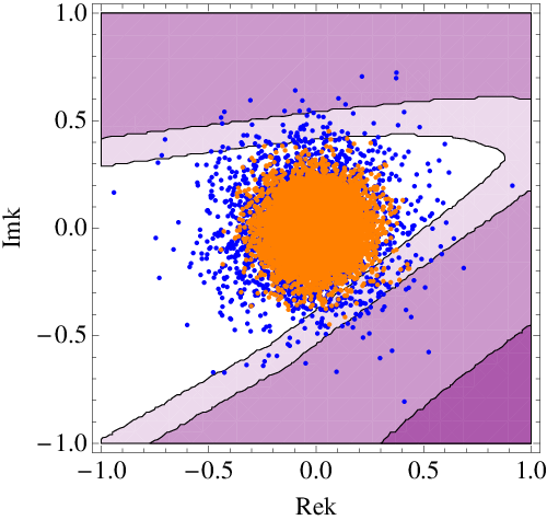
with a generic squark mass $m_{\tilde{q}}$ . The remaining flavour-conserving elements are specified by $\hat{m}_{\tilde{u}}^{2}=\text{Diag}(m_{\tilde{q}}^{2},m_{\tilde{q}}^{2},m_{\tilde{t}_{R}}^{2})$ , $(\hat{T}_{U})_{ii}=(\hat{T}_{U})_{33}\delta_{i3}$ and $\tan\beta=10$ .

We have performed a scan over the free parameters in the value ranges defined in the table in fig. 10 to identify possible sources of large isospin-violation. In fig. 9 we plot the Z-penguin contribution to $|q_{7}|$ and $|q_{9}|$ ( $q_{i}$ is defined in eq. (31)) over the sum of all contributions to $|q_{7}|$ and $|q_{9}|$ for 30000 random points. We see that considering the Z-penguin only is a very good approximation for all points yielding large isospin-violation. In this way our scenario is essentially equivalent to the one with a left-handed flavour-changing Z coupling $\kappa_{L}^{sb}$ discussed in sec. 4.2 and we will stay in this approximation in the following. Since a non-vanishing $\kappa_{L}^{sb}$ breaks electroweak symmetry [74] it must involve the vacuum expectation values $v_{u,d}$ . Therefore it is almost exclusively sensitive to $\delta_{32}^{uRL}$ and not to $\delta_{32}^{uLL}$ and we will neglect the latter in the following.

Having calculated the MSSM mass spectrum for a given parameter point we apply the following constraints:

•

physical squark and chargino masses $\geq 100$ GeV ,
•

${\rm Br}(\bar{B}\to X_{s}\gamma)$ compatible with data at the $2\sigma$ level,
•

chargino contribution $|C^{\chi}_{7\gamma}|\leq|C^{\text{SM}}_{7\gamma}|\approx 0.22$ .

The last constraint ensures that fine-tuned points passing the ${\rm Br}(\bar{B}\to X_{s}\gamma)$ constraint are not considered.

It has been suggested [82] that a non-vanishing $\delta_{32}^{uRL}$ can generate isospin-violating effects large enough to explain the $\Delta A_{\text{CP}}$ discrepancy within the QCDF framework. This would clearly be an interesting perspective for supersymmetric effects in purely isospin-violating decays. However, we cannot confirm this statement in our framework. In fig. 9 we find that $C_{9}$ can be enhanced by about 25% and $C_{7}$ by about 8% with respect to the SM in the presence of a non-vanishing $\delta_{32}^{uRL}$ ^†^† † Including the naturalness constraint $|\delta_{32}^{uRL}|<0.59$ [86] the effects become even smaller.. In section 3 we have seen that a 25% effect in $C_{9}$ or an 8% effect in $C_{7}$ are not enough to generate a large $\Delta A_{\text{CP}}$ and are also not sufficient to enhance the branching fractions of $\bar{B}_{s}\rightarrow\phi\pi^{0}$ and $\bar{B}_{s}\rightarrow\phi\rho^{0}$ sizeably. A NP effect of this size would be hidden in the theoretical uncertainty and thus be unobservable. These findings are illustrated in figs. 10 and 11, where we display on the one hand a figure similar to fig. 3 in the complex $\kappa_{L}^{sb}$ plane and on the other hand a zoomed version of the upper plots in fig. 6. To both figures we add the $\kappa_{L}^{sb}$ values resulting from chargino-induced flavour-violating Z couplings in a scan over 30000 points in the MSSM parameter space as defined in the table in fig. 10 to illustrate the statements of the last paragraph.

We note that there is an important difference between our calculation and the one of [82], namely the treatment of strong phases. We obtain all of these phases directly from QCDF, where they are suppressed by either $\alpha_{s}(m_{b})$ or $\Lambda_{\text{QCD}}/m_{B}$ . Thus we typically find small strong phases even though their prediction comes with a large uncertainty. In the framework of ref. [82] only absolute values of penguin-to-tree ratios are predicted from QCDF whereas the corresponding strong phases can assume arbitrary values between $0$ and $\pi$ [87]. In this way, large CP asymmetries can be generated even without a large NP contribution and also the fact that $A_{\rm CP}(B^{-}\to\pi^{0}K^{-})$ and $A_{\rm CP}(\bar{B}^{0}\to\pi^{+}K^{-})$ have opposite sign is no longer puzzling because the phases of the various tree and penguin topologies are uncorrelated. In contrast, our calculation reduces the $2.5\sigma$ SM discrepancy in $\Delta A_{\text{CP}}$ only marginally. From fig. 10 we can read off that the vast majority of the allowed points are outside the $2.2\sigma$ region. Only a few rather fine-tuned points are between $2.2\sigma$ and $2\sigma$ .

5 Conclusion

In this article we have studied the possibility of probing isospin-violating NP in hadronic $B$ decays. We have proposed to test the EW penguin sector of the effective weak Hamiltonian via the decays $\bar{B}_{s}\to\phi\pi^{0}$ and $\bar{B}_{s}\to\phi\rho^{0}$ and provided a detailed phenomenological analysis of these two modes in correlation to other hadronic $B$ decays.

Our analysis is motivated by discrepancies found in $B\to\pi K$ decays, which are to date the best-measured hadronic $b\rightarrow s$ decays. In particular, the $2.5\,\sigma$ discrepancy found in the observable $\Delta A_{\rm CP}$ can be interpreted as a sign of NP in the EW penguin sector of the theory. We have demonstrated in a model-independent analysis that this discrepancy can easily be resolved by an additional NP contribution to the EW penguin operators $Q_{7}^{(\prime)},...,Q_{10}^{(\prime)}$ if it is of the same order of magnitude as the leading SM coefficient $C_{9}^{\textrm{SM}}$ . An exception are parity-symmetric scenarios where the contributions to $PP$ decays cancel. Whereas the solution in the case of NP in $C_{9}^{(\prime)}$ is, as expected, due to a new contribution to the colour-allowed EW penguin amplitude, we have pointed out that, in the case of NP in $C_{7}^{(\prime)}$ , the solution mainly comes about via a weak annihilation contribution in the QCDF framework which has a surprisingly large imaginary part. In particular we have found for the case of equal new contributions to $C_{7}$ and $C_{9}$ that, even though these contributions tend to cancel in the EW penguin amplitude, the $\Delta A_{CP}$ discrepancy can still be solved via the EW penguin annihilation amplitude, a fact that had not been noticed before. For various scenarios we have performed frequentist fits to $B\to\pi K$ data. We have found the fit to work well for NP in $C_{9}^{(\prime)}$ while NP in $C_{7}^{(\prime)}$ is only poorly constrained from $B\to\pi K$ alone. Especially in this case, the $PV$ counterparts $B\to\rho K$ and $B\to\pi K^{*}$ , which carry a different interplay of chiralities, give valuable additional information. We have seen that present experimental data already set strong constraints: a new EW penguin amplitude can be at most $\sim 5$ times larger than the SM one; on the other hand a new amplitude of about the same size as the SM one is required to solve the $\Delta A_{CP}$ discrepancy.

Whether the discrepancy in $\Delta A_{\rm CP}$ really is a manifestation of NP, however, is not clear because the experimental data are still not conclusive due to the large uncertainties in the theory prediction and the still somewhat low statistics of the measurements. The long-standing problem of large theoretical hadronic uncertainties in hadronic decays can, however, be partially addressed exploiting the large variety of hadronic decay channels. In the case at hand, the best test is provided by the $\bar{B}_{s}\to\phi\pi^{0}$ and $\bar{B}_{s}\to\phi\rho^{0}$ modes, which are purely isospin-violating decays and are dominated by the EW penguin amplitude. Since these decays are not related to other hadronic $B$ decays via flavour symmetries, their analysis requires a determination of the hadronic matrix elements from first principles and we used the QCDF approach to this end. From the full QCDF results we have derived simple approximate expressions (eqs. (21)-(23), (33)) which reproduce the $\bar{B}_{s}\to\phi\pi^{0},\phi\rho^{0}$ amplitudes with high accuracy for arbitrary scenarios with NP in $C_{7}^{(\prime)},...,C_{10}^{(\prime)}$ . By quoting these formulae we facilitate the study of these decays without an extensive implementation of the QCDF framework.

In this work we have performed the first analysis of the impact of NP in EW penguins on $\bar{B}_{s}\to\phi\pi^{0},\phi\rho^{0}$ . A new EW penguin amplitude of the same size as the SM one can easily enhance the $\bar{B}_{s}\to\phi\pi^{0}$ and $\bar{B}_{s}\to\phi\rho^{0}$ branching ratios by an order of magnitude. We have performed a quantitative analysis parameterising NP in EW penguins in a model-independent way, at the level of Wilson coefficients, and studied the maximum enhancement of the $\bar{B}_{s}\to\phi\pi^{0},\phi\rho^{0}$ branching ratios for various scenarios, with respect to the result of our $B\to K\pi$ fits and with respect to constraints from other hadronic $B$ decays. The results displayed in tab. 3 show that in many cases a large enhancement is possible. Particular exceptions are parity-symmetric models which have no impact on the $VV$ decay $\bar{B}_{s}\to\phi\rho^{0}$ and scenarios with (approximately) equal contributions to $C_{7}^{(\prime)}$ and $C_{9}^{(\prime)}$ which cancel in $\bar{B}_{s}\to\phi\pi^{0}$ .

A survey of concrete NP models has been performed in section 4, where we have considered a modified $Z^{0}$ penguin, a model with an additional $U(1)^{\prime}$ gauge symmetry and the MSSM. In such models additional constraints arise from the semileptonic decays $\bar{B}\to X_{s}e^{+}e^{-}$ and $\bar{B}\to K^{*}l^{+}l^{-}$ and from $B_{s}$ - $\bar{B}_{s}$ mixing. In case of the modified- $Z^{0}$ -penguin scenario we have found that the semileptonic constraints still allow for NP to an extent which is sufficient to resolve the $\Delta A_{\textrm{CP}}$ discrepancy. On the other hand, they prevent the $\bar{B}_{s}\to\phi\pi^{0},\phi\rho^{0}$ decays from developing an enhancement which beats the hadronic uncertainties of the SM prediction. Therefore, a large effect measured in these decays would rule out the modified $Z$ coupling. The semileptonic constraints can for example be avoided in a model with an additional $Z^{\prime}$ boson whose couplings to leptons can be switched off. Our analysis has shown that in this scenario constraints from hadronic $B$ decays and $B_{s}$ - $\bar{B}_{s}$ mixing can be fulfilled simultaneously only at the $2\,\sigma$ level. The tight constraints from $B_{s}$ - $\bar{B}_{s}$ mixing limit a potential enhancement of $\bar{B}_{s}\to\phi\pi^{0},\phi\rho^{0}$ to a factor $\sim 5$ . Furthermore the occurrence of such a measurable enhancement requires a large $g_{U(1)^{\prime}}$ coupling and/or a light $Z^{\prime}$ boson. Finally our conclusion for the MSSM is that it is impossible to obtain a new contribution larger than about 25% in $C_{9}$ and about 8% in $C_{7}$ , which is clearly not enough to generate a large $\Delta A_{\text{CP}}$ or a significant enhancement of the $B_{s}$ decays. The $\Delta A_{\text{CP}}$ discrepancy can be reduced only marginally in this way. Only a few rather fine-tuned parameter points reduce it from $2.5\sigma$ to $2\sigma$ .

We stress again that the decays $\bar{B}_{s}\to\phi\pi^{0},\phi\rho^{0}$ are highly sensitive to isospin-violating NP. Their measurement would complement the analysis of $B\to K\pi$ decays and could shed light on the “ $\Delta A_{\textrm{CP}}$ puzzle”. For this reason we strongly encourage experimental efforts to measure these decays at LHCb and at future Super-B factories.

Acknowledgements

We would like to thank U. Nierste for initiating the project and for a careful reading of the manuscript. We are grateful to him and to M. Beneke for useful discussions and suggestions. Furthermore we thank A. Crivellin for helpful discussions on chirally enhanced corrections in SUSY, and S. Khalil for helpful communications on [81] and [82]. This work is supported by the DFG Sonderforschungsbereich/Transregio 9 “Computergestützte Theoretische Teilchenphysik” and by the EU contract No. MRTN-CT-2006-035482, “FLAVIAnet”. L.V. acknowledges the TTP Karlsruhe and the CERN Theory group for hospitality, and the Alexander-von-Humboldt Foundation for support. L.H. and D.S. acknowledge the support by Ev. Studienwerk Villigst and by Cusanuswerk, respectively, and by the DFG Graduate College High Energy Physics and Particle Astrophysics. L.H. is further supported by the Federal Ministry of Education and Research (BMBF) under constract No. 05H09WWE.

Appendix A General framework for the calculation of hadronic $B$ decays

Throughout this work, we study hadronic B decays into two light mesons using the framework of QCD factorisation [13, 14, 15, 16, 17]. This framework is based on the well-known effective weak Hamiltonian for $\Delta B=1$ transitions given in (5) and described in section A.1. Matrix elements of this Hamiltonian are calculated in an expansion in $\Lambda_{\text{QCD}}/m_{B}$ . We give a few details concerning the generalisation of QCDF to a Hamiltonian containing operators with flipped chiralities in section A.2 and specify our input parameters in section A.3. In section A.4 we collect expressions for obtaining various observables from the QCDF-calculated amplitudes.

A.1 The effective weak Hamiltonian

The starting point for the analysis of hadronic B decays is the parameterisation of high-energy transitions in terms of effective four-quark operators multiplied by short-distance coefficients. In the SM, this leads to the effective weak Hamiltonian in eq. (5). The short-distance coefficients $C_{i}$ are calculated in the $\overline{\text{MS}}$ renormalisation scheme at the scale $\mu_{\rm EW}\sim M_{W}$ . Their low-scale values at $\mu_{\rm EW}\sim m_{b}$ are obtained from renormalisation-group equations (RGE). In the SM, only $C_{1}$ is ${\cal O}(1)$ , while $C_{2}$ and the QCD penguin coefficients $C_{3,\ldots,6}$ arise at order $\mathcal{O}(\alpha_{s})$ and the electroweak penguin coefficients arise at order $\mathcal{O}(\alpha)$ , albeit partly enhanced by factors of $x_{tW}=m^{2}_{t}/m^{2}_{W}$ and/or $1/\sin^{2}\theta_{W}$ . The complete analytical expressions for these coefficients are written down e.g. in [66].

Besides the SM operators, we also consider the possibility that New Physics gives rise to the so-called “mirror” penguin operators $Q^{\prime}_{i}$ , obtained from $Q_{i}$ by a global exchange of left- and right-handed chiralities of the quark fields, $(V-A)\leftrightarrow(V+A)$ . We thus replace in eq. (5)

C_{i}Q_{i}\longrightarrow C_{i}Q_{i}+C^{\prime}_{i}Q^{\prime}_{i}.

(58)

Given the enhancement of $C_{7}(\mu_{\rm EW})$ and $C_{9}(\mu_{\rm EW})$ by $x_{tW}$ and/or $1/\sin^{2}\theta_{W}$ , we follow the modified RGE scheme presented in [15] for the SM coefficients and consider the enhanced terms as leading-order coefficients, i.e.

C_{7}^{\text{LO}}(M_{W})=\frac{\alpha}{4\pi}\frac{x_{tW}}{3}\hskip 11.49994pt,\hskip 11.49994ptC_{9}^{\text{LO}}(M_{W})=\frac{\alpha}{4\pi}\left[\frac{x_{tW}}{3}+\frac{2}{3\sin^{2}\theta_{W}}(10B_{0}(x_{tW})-4C_{0}(x_{tW}))\right]

(59)

with the loop functions $B_{0}(x)$ and $C_{0}(x)$ from [66]. To be consistent we neglect at the same time electromagnetic corrections to the QCD penguin coefficients as well as any mixing of $C_{7},\ldots,C_{10}$ into $C_{1},...,C_{6}$ . Since this treatment improves the RGE evolution for $C_{7},...,C_{10}$ and since it is exactly these coefficients we are interested in, it is well suited for our analysis. By contrast, for the NP contributions we use the standard treatment for the leading-order RGE.

A.2 Operator matrix elements in QCDF

From the effective Hamiltonian (5) the decay amplitude for the process $\bar{B}\rightarrow M_{1}M_{2}$ can be calculated as

\mathcal{A}^{(h)}_{\bar{B}\rightarrow M_{1}M_{2}}\,=\,\langle M_{1}^{(h)}M_{2}^{(h)}|{\cal{H}_{\rm eff}}|\bar{B}\rangle,

(60)

where $h$ refers to a helicity amplitude in case of a decay into two vector mesons, $\bar{B}\to V_{1}^{h}V_{2}^{h}$ with $h=0,+,-$ .

In QCDF the matrix elements of the effective Hamiltonian are organised in terms of flavour amplitudes $\alpha_{i}$ which are directly related to the topologies of the underlying weak transition, for example colour-allowed EW penguin, colour-suppressed tree etc. Analogous amplitudes $\beta_{i}$ represent the corresponding weak annihilation transitions. The topological amplitudes $\alpha_{i}$ in turn can be decomposed into coefficients $a_{i}$ which are in direct correspondence to the operators $Q_{i}$ in the effective Hamiltonian. At NLO these coefficients $a_{i}$ contain the perturbative non-factorisable vertex-, penguin- and spectator-scattering corrections governed by the factorisation formula. For a complete description we refer to [16]. The expressions given there can easily be generalised to account for the mirror operators by adding a topological amplitude $\alpha_{i}^{\prime}$ to each of the $\alpha_{i}$ [88]. A similar generalisation applies to the annihilation amplitudes $\beta_{i}$ . Here we only need to add the expressions for $\alpha_{3\rm EW,4EW}^{\prime}$ , which read

	$\displaystyle\alpha^{\prime\,p}_{\rm 3EW}(M_{1}M_{2})$	$\displaystyle=$	$\displaystyle\left\{\begin{array}[]{cl}-a^{\prime\,p}_{9}(M_{1}M_{2})+a^{\prime\,p}_{7}(M_{1}M_{2}),&\hskip 11.49994pt\mbox{if~}M_{1}M_{2}=PP,\\ a^{\prime\,p}_{9}(M_{1}M_{2})+a^{\prime\,p}_{7}(M_{1}M_{2}),&\hskip 11.49994pt\mbox{if~}M_{1}M_{2}=PV,\\ a^{\prime\,p}_{9}(M_{1}M_{2})-a^{\prime\,p}_{7}(M_{1}M_{2}),&\hskip 11.49994pt\mbox{if~}M_{1}M_{2}=VP,\\ -a^{\prime\,p}_{9}(M_{1}M_{2})-a^{\prime\,p}_{7}(M_{1}M_{2}),&\hskip 11.49994pt\mbox{if~}M_{1}M_{2}=V^{0}V^{0},\\ -f^{M_{1}}_{\pm}\left(a^{\prime\,p}_{9}(M_{1}M_{2})+a^{\prime\,p}_{7}(M_{1}M_{2})\right),&\hskip 11.49994pt\mbox{if~}M_{1}M_{2}=V^{\pm}V^{\pm},\end{array}\right.$
	$\displaystyle\alpha^{\prime\,p}_{\rm 4EW}(M_{1}M_{2})$	$\displaystyle=$	$\displaystyle\left\{\begin{array}[]{cl}-a^{\prime\,p}_{10}(M_{1}M_{2})-r_{\chi}^{M_{2}}\,a^{\prime\,p}_{8}(M_{1}M_{2}),&\hskip 11.49994pt\mbox{if~}M_{1}M_{2}=PP,\\ a^{\prime\,p}_{10}(M_{1}M_{2})+r_{\chi}^{M_{2}}\,a^{\prime\,p}_{8}(M_{1}M_{2}),&\hskip 11.49994pt\mbox{if~}M_{1}M_{2}=PV,\\ a^{\prime\,p}_{10}(M_{1}M_{2})-r_{\chi}^{M_{2}}\,a^{\prime\,p}_{8}(M_{1}M_{2}),&\hskip 11.49994pt\mbox{if~}M_{1}M_{2}=VP,\\ -a^{\prime\,p}_{10}(M_{1}M_{2})+r_{\chi}^{M_{2}}\,a^{\prime\,p}_{8}(M_{1}M_{2}),&\hskip 11.49994pt\mbox{if~}M_{1}M_{2}=V^{0}V^{0},\\ f^{M_{1}}_{\pm}\left(-a^{\prime\,p}_{10}(M_{1}M_{2})+r_{\chi}^{M_{2}}\,a^{\prime\,p}_{8}(M_{1}M_{2})\right),&\hskip 11.49994pt\mbox{if~}M_{1}M_{2}=V^{\pm}V^{\pm}\end{array}\right.$

with $f^{M_{1}}_{\pm}=F_{\mp}^{B\rightarrow M_{1}}(0)/F_{\pm}^{B\rightarrow M_{1}}(0)$ being a ratio of form factors, such that $f^{M_{1}}_{+}\sim m_{B}/\Lambda_{\rm QCD}$ and $f^{M_{1}}_{-}\sim\Lambda_{\rm QCD}/m_{B}$ in the heavy-quark limit [17]. The NLO expressions for the coefficients $a_{i}^{\prime}$ are equivalent to the ones for the coefficients $a_{i}$ from [16] up to the replacement $C_{i}\rightarrow C_{i}^{\prime}$ . Additionally in the transverse amplitudes of $B\to VV$ decays one has to flip the helicities, i.e. the expressions for $a_{i}^{+}$ are needed for ${a_{i}^{\prime}}^{-}$ and vice versa.

The pattern of signs appearing in eq. (A.2) is a consequence of the fact that matrix elements of the mirror operators are related to the SM ones by parity

\langle M_{1}M_{2}|Q_{i}|\bar{B}\rangle\,=\,-\eta_{M_{1}M_{2}}\,\langle M_{1}M_{2}|Q_{i}^{\prime}|\bar{B}\rangle,

(73)

which implies that the amplitudes involve the coefficients $a_{i}^{(\prime)}$ only in the combinations [56]

a^{p}_{i}(M_{1},M_{2})\,-\,\eta_{M_{1}M_{2}}\,a^{\prime\,p}_{i}(M_{1},M_{2}).

(74)

Here $\eta_{M_{1}M_{2}}=\pm 1$ is the parity of the final state. For $PP$ and longitudinal $VV$ final states, we have $\eta_{M_{1}M_{2}}=1$ whereas for $PV$ final states $\eta_{M_{1}M_{2}}=-1$ . In this manner left-handed and right-handed NP give rise to different signatures and correlations among $PP$ , $PV$ or $VV$ decays. Exploiting this feature can be very important in order to probe the chirality structure of a potential NP model.

A.3 Input parameters and tree to penguin ratios in $B\to\pi K$ , $B\to\pi\pi$

QCD scale and running quark masses [GeV]
$\Lambda_{\overline{\rm MS}}^{(5)}$	$m_{b}(m_{b})$	$m_{c}(m_{b})$	$m_{s}$	$m_{q}/m_{s}$
0.231	4.2	1.3 $\pm$ 0.2	0.090 $\pm$ 0.020	0.0413
CKM parameters
$\lambda$	$\|V_{cb}\|$	$\|V_{ub}/V_{cb}\|$	$\gamma$	$\sin(2\beta)$
$0.225$	$0.0415\pm 0.0010$	$0.085^{+0.025}_{-0.015}$	$(70\pm 10)^{\circ}$	$0.673\pm 0.23$
B meson parameters
		$B^{-}$	$\bar{B}^{0}$	$\bar{B}_{s}^{0}$
Lifetime	$\tau$ [ps]	$1.638$	$1.525$	$1.472$
Decay constant	$f_{B}$ [MeV]	$210\pm 20$		$240\pm 20$
	$\lambda_{B}$ [MeV]	$200^{+250}_{-0}$		$200^{+250}_{-0}$

Pseudoscalar-meson decay constants and Gegenbauer moments
	$\pi$	$K$
$f$ [MeV]	$131$	$160$
$\alpha_{1},\alpha_{1,\perp}$	$0$	$0.06\pm 0.06$
$\alpha_{2},\alpha_{2,\perp}$	$0.20\pm 0.15$	$0.20\pm 0.15$

Vector-meson decay constants and Gegenbauer moments
	$\rho$	$K^{*}$	$\phi$
$f$ [MeV]	$209\pm 1$	$218\pm 4$	$221\pm 3$
$f^{\perp}$ [MeV]	$165\pm 9$	$185\pm 10$	$186\pm 9$
$\alpha_{1},\alpha_{1,\perp}$	$0$	$0.06\pm 0.06$	$0$
$\alpha_{2},\alpha_{2,\perp}$	$0.1\pm 0.2$	$0.1\pm 0.2$	$0\pm 0.3$
Pseudoscalar-meson form factor at $q^{2}=0$
	$B\to\pi$	$B\to K$	$B_{s}\to\bar{K}$
$F_{0}$	$0.25\pm 0.05$	$0.34\pm 0.05$	$0.31\pm 0.05$
Vector-meson form factor at $q^{2}=0$
	$B\to\rho$	$B\to K^{*}$	$B_{s}\to\phi$
$A_{0}$	$0.30^{+0.07}_{-0.03}$	$0.39\pm 0.06$	$0.38^{+0.10}_{-0.02}$
$F_{+}$	$0.00\pm 0.06$	$0.00\pm 0.06$	$0.00\pm 0.06$
$F_{-}$	$0.55\pm 0.06$	$0.68\pm 0.07$	$0.65^{+0.14}_{-0.00}$

Table 8: Summary of the theoretical input parameters for hadronic

B

decays into two light mesons. All scale-dependent quantities refer to

\mu=2\,\mbox{GeV}

unless otherwise stated. The values represent the most up-to-date values taken from [16, 17, 89, 90, 91, 92, 93].

In the framework of QCDF the decay amplitudes depend on quite a few input parameters such as form factors, Gegenbauer moments of light-cone distribution amplitudes, etc. In tab. 8 we provide a list of up-to-date values. We use the updated value of $\Lambda_{\overline{\rm MS}}^{(5)}$ as obtained in [94]; as of $\lambda_{B}=\lambda_{B_{s}}$ we assume the lower value 200 MeV as suggested by exclusive hadronic decays, see [17, 90, 92, 95]. Particular attention deserves the choice of $X_{H,A}$ , i.e. the numbers which parameterise our ignorance of non-perturbative physics occurring in spectator scattering and weak annihilation due to the exchange of soft gluons. For $X_{H}$ we use the definition of [16],

X_{H}=(1+\rho_{H}e^{i\phi_{H}})\ln\frac{m_{B}}{\Lambda_{h}},

(75)

with a non-perturbative scale $\Lambda_{h}=500$ MeV. The default value is $\rho_{H}=0$ and we estimate the uncertainty setting $\rho_{H}=1$ and freely varying $\phi_{H}$ between $0$ and $2\pi$ . In the light of experimental data, $X_{A}$ requires more attention. The reasoning goes as follows.

A good test of the QCDF hypothesis is to look at the $\pi K$ -penguin to $\pi\pi$ -tree ratio [16], which can be directly related to experimental observables:

\left|\frac{\hat{\alpha}_{4}^{c}(\pi\bar{K})}{\alpha_{1}(\pi\pi)+\alpha_{2}(\pi\pi)}\right|\simeq\left|\frac{V_{ub}}{V_{cb}}\right|\frac{f_{\pi}}{f_{K}}\left[\frac{\Gamma(B^{-}\to\pi^{-}\bar{K}^{0})}{\Gamma(B^{-}\to\pi^{-}\pi^{0})}\right]^{1/2}\stackrel{{\scriptstyle\text{exp.}}}{{=}}0.100^{+0.030}_{-0.018}.

(76)

To a good approximation this ratio relates a pure QCD-penguin decay to a pure tree decay and allows to eliminate the uncertainty from the heavy-to-light form factor. Since the tree decay $B^{-}\to\pi^{-}\pi^{0}$ suffers from small uncertainties in QCDF and is expected to receive negligible contributions from NP, eq. (76) probes the accuracy of the QCDF prediction for the penguin amplitude $\hat{\alpha}_{4}^{c}(\pi\bar{K})$ . In absence of sizeable NP contributions to QCD penguins it constrains the uncalculable weak-annihilation contribution $\beta_{3}^{c}$ , which is responsible for the lion’s share of the theoretical uncertainty in the penguin amplitude. Though subleading in $\Lambda_{\rm QCD}/m_{B}$ , $\beta_{3}^{c}$ is known to be numerically enhanced.

Using the parameters in tab. 8 and expressing $\beta_{3}^{c}$ via the complex ${\cal O}(1)$ parameter $X_{A}$ as in ref. [16] with

X_{A}=(1+\rho_{A}e^{i\phi_{A}})\ln\frac{m_{B}}{\Lambda_{h}}

(77)

with the default value $\rho_{A}=0$ , we find

\left|\frac{\hat{\alpha}_{4}^{c}(\pi\bar{K})}{\alpha_{1}(\pi\pi)+\alpha_{2}(\pi\pi)}\right|\stackrel{{\scriptstyle\text{SM}}}{{=}}0.078^{+0.025}_{-0.015},

(78)

which is slightly smaller than older results. Repeating the analysis of [16] for the $PV$ and $VV$ modes we obtain fig. 12. The plots show the experimental central values and uncertainties of the ratio in eq. (76) (circles around the origin) for $B\rightarrow\pi K$ and three related decays. They are combined with “limaçon” curves representing the corresponding theory predictions where the phase $\phi_{A}$ is freely varied between $0$ and $2\pi$ while we set $\rho_{A}=1$ $(1.5,2)$ for $PP$ and $PV$ modes and $\rho_{A}=0.6$ $(1.0,1.5)$ for $VV$ modes to obtain the blue (purple, yellow) curves. The red dots correspond to $\rho_{A}=0,1,1.5$ ( $\rho_{A}=0,0.6,1.0$ for $VV$ modes) with $\phi_{A}$ fixed as in the scenario “S4” in [16] for $PP$ and $PV$ modes and $\phi_{A}=-40^{\circ}$ for $VV$ .

These results lead us to the conclusion that, in the light of present data, we prefer to change the widely used treatment with $\rho_{A}=0$ as default and $\rho_{A}=1$ ( $\rho_{A}=0.6$ for $VV$ ) for the variation of $\phi_{A}$ in order to have a more conservative estimate of the theoretical uncertainty. Nevertheless we confirm that $\rho_{A}\leq 2$ is a reasonable upper bound for weak-annihilation contributions in QCDF. We adopt $\rho_{A}=1.5$ ( $\rho_{A}=1.0$ for $VV$ modes) as our default value, keeping the default for $\phi_{A}$ as above, and estimate the uncertainty with $\rho_{A}$ unchanged and $\phi_{A}\in[0,2\pi)$ .

A.4 Calculating observables in hadronic $B$ decays

Starting from a decay amplitude $\mathcal{A}(\bar{B}\to M_{1}M_{2})$ the corresponding decay rate can be calculated as

\Gamma(\bar{B}\to M_{1}M_{2})=\frac{S}{16\pi m_{B}}|\mathcal{A}(\bar{B}\to M_{1}M_{2})|^{2},

(79)

with a symmetry factor $S$ . We have $S=1/2$ if $M_{1}$ and $M_{2}$ are identical and $S=1$ otherwise. For decays into two vector mesons, where three different helicity amplitudes exist, one replaces $|\mathcal{A}(\bar{B}\to M_{1}M_{2})|^{2}$ by a sum over the three possible helicities of the final state, $\sum_{h=0,-,+}|\mathcal{A}^{h}(\bar{B}\to V_{1}V_{2})|^{2}$ . The branching ratios are easily calculated from ${\rm Br}(\bar{B}\to M_{1}M_{2})=\Gamma(\bar{B}\to M_{1}M_{2})/\Gamma_{\rm tot}$ with $\Gamma_{\rm tot}$ being the total decay width of the $\bar{B}$ meson. Our theoretical predictions always refer to CP-averaged branching ratios defined as

\overline{{\rm Br}}(\bar{B}\to\bar{f})=\frac{1}{2}\left({\rm Br}(\bar{B}\to\bar{f})+{\rm Br}(B\to f)\right),

(80)

where $\bar{f},f$ stand for the final state $M_{1}M_{2}$ and its CP-conjugated state. The CP-conjugated decay rate is calculated by replacing $\mathcal{A}$ in eq. (79) by the corresponding CP-conjugated amplitude. This amounts to a change of sign for all the weak phases while strong phases are unchanged.

The direct CP asymmetries read

A_{\rm CP}=\frac{{\rm Br}(\bar{B}\to\bar{f})-{\rm Br}(B\to f)}{{\rm Br}(\bar{B}\to\bar{f})+{\rm Br}(B\to f)}

(81)

and the longitudinal polarisation fraction $f_{L}(\bar{B}\to M_{1}M_{2})$ is defined as

f_{L}(\bar{B}\to M_{1}M_{2})=\frac{|\mathcal{A}^{0}(\bar{B}\to V_{1}V_{2})|^{2}}{\sum_{h=0,-,+}|\mathcal{A}^{h}(\bar{B}\to V_{1}V_{2})|^{2}}.

(82)

Appendix B Isospin-violating observables in $B\to\pi K$

In this appendix we present the observables which are sensitive to isopin violation in the $B\to\pi K$ decay modes and which we use to calculate our $2\,\sigma$ constraints.

First, one has ratios of any two different decay rates. Using the parameterisation (10) and neglecting terms which are quadratic in the $r_{i}$ as well as the annihilation contribution $r_{\textrm{EW}}^{\textrm{A}}$ which has only a small real part, one has 6 different ratios which read [10, 11]

$\displaystyle R_{c}^{B}$	$\displaystyle\equiv$	$\displaystyle 2\,\frac{\overline{{\rm Br}}(B^{-}\to\pi^{0}K^{-})}{\overline{{\rm Br}}(B^{-}\to\pi^{-}\bar{K}^{0})}\,\simeq\,1\,+\,2\,{\rm Re}(r_{\textrm{EW}}+r_{\textrm{EW}}^{\textrm{C}})-\,2\,{\rm Re}(r_{\textrm{T}}+r_{\textrm{C}})\cos\gamma\,,$
$\displaystyle R_{n}^{B}$	$\displaystyle\equiv$	$\displaystyle\frac{1}{2}\,\frac{\overline{{\rm Br}}(\bar{B}^{0}\to\pi^{+}K^{-})}{\overline{{\rm Br}}(\bar{B}^{0}\to\pi^{0}\bar{K}^{0})}\,\simeq\,1\,+\,2\,{\rm Re}(r_{\textrm{EW}}+r_{\textrm{EW}}^{\textrm{C}})-\,2\,{\rm Re}(r_{\textrm{T}}+r_{\textrm{C}})\cos\gamma\,,$
$\displaystyle R_{c}^{K}$	$\displaystyle\equiv$	$\displaystyle 2\,\frac{\tau_{0}}{\tau_{-}}\,\frac{\overline{{\rm Br}}(B^{-}\to\pi^{0}K^{-})}{\overline{{\rm Br}}(\bar{B}^{0}\to\pi^{+}K^{-})}\,\simeq\,1\,+\,2\,{\rm Re}(r_{\textrm{EW}})-\,2\,{\rm Re}(r_{\textrm{C}})\cos\gamma\,,$
$\displaystyle R_{n}^{K}$	$\displaystyle\equiv$	$\displaystyle\frac{1}{2}\,\frac{\tau_{0}}{\tau_{-}}\,\frac{\overline{{\rm Br}}(B^{-}\to\pi^{-}\bar{K}^{0})}{\overline{{\rm Br}}(\bar{B}^{0}\to\pi^{0}\bar{K}^{0})}\,\simeq\,1\,+\,2\,{\rm Re}(r_{\textrm{EW}})-\,2\,{\rm Re}(r_{\textrm{C}})\cos\gamma\,,$
$\displaystyle R_{c}^{\pi}$	$\displaystyle\equiv$	$\displaystyle\frac{\tau_{0}}{\tau_{-}}\frac{\overline{{\rm Br}}(B^{-}\to\pi^{-}\bar{K}^{0})}{\overline{{\rm Br}}(\bar{B}^{0}\to\pi^{+}K^{-})}\,\simeq\,1\,+\,2\,{\rm Re}(r_{\textrm{T}})\cos\gamma-\,2\,{\rm Re}(r_{\textrm{EW}}^{\textrm{C}}),$
$\displaystyle R_{n}^{\pi}$	$\displaystyle\equiv$	$\displaystyle\frac{\tau_{0}}{\tau_{-}}\,\frac{\overline{{\rm Br}}(B^{-}\to\pi^{0}K^{-})}{\overline{{\rm Br}}(\bar{B}^{0}\to\pi^{0}\bar{K}^{0})}\,\simeq\,1-\,2\,{\rm Re}(r_{\textrm{T}}+2r_{\textrm{C}})\cos\gamma\,+\,2\,{\rm Re}(2r_{\textrm{EW}}+r_{\textrm{EW}}^{\textrm{C}})\,,\hskip 14.22636pt$	(83)

where $\tau_{0}$ and $\tau_{-}$ are the lifetimes of the neutral and charged $B$ mesons, respectively. NP in EW penguins as in (13) enters the ratios $R_{c,n}^{B,K,\pi}$ through

	$\displaystyle{\rm Re}(r_{\text{EW}})$	$\displaystyle\rightarrow$	$\displaystyle{\rm Re}(r_{\text{EW}})+{\rm Re}(\tilde{r}_{\text{EW}})\cos\delta,$
	$\displaystyle{\rm Re}(r_{\text{EW}}^{\textrm{C}})$	$\displaystyle\rightarrow$	$\displaystyle{\rm Re}(r_{\text{EW}}^{\textrm{C}})+{\rm Re}(\tilde{r}_{\text{EW}}^{\textrm{C}})\cos\delta.$		(84)

Experimental data on the $R_{c,n}^{B,K,\pi}$ can be used to constrain the NP contributions $\tilde{r}_{\text{EW}}$ and $\tilde{r}_{\text{EW}}^{\textrm{C}}$ . Note that the $R_{c,n}^{B,K,\pi}$ involve different combinations of $\tilde{r}_{\text{EW}}$ and $\tilde{r}_{\text{EW}}^{\textrm{C}}$ and thus they are sensitive to different linear combinations of the electroweak penguin coefficients $C_{7}^{(\prime)},...,C_{10}^{(\prime)}$ . Therefore, it depends on the specific NP scenario in consideration which of the $R_{c,n}^{B,K,\pi}$ give the best constraints.

Beyond being responsible for the universal QCD penguin contribution, isospin relations account for the approximate equation

\Gamma(B^{-}\to\pi^{-}\bar{K}^{0})-2\,\Gamma(B^{-}\to\pi^{0}K^{-})\,\approx\,2\,\Gamma(\bar{B}^{0}\to\pi^{0}\bar{K}^{0})-\Gamma(\bar{B}^{0}\to\pi^{+}K^{-})

(85)

known as Lipkin sum rule [96]. In the strict isospin limit both sides of this equation vanish identically. This is reflected in the fact that $R^{B}_{c,n}$ in (83) are both equal to one, apart from isospin-violating terms of order $\mathcal{O}(r_{i})$ . These linear terms are generated by the interference of the isospin-violating parts of the amplitude with the QCD penguin part. The special property of (85) is now that these interference terms on the left- and righthand side of the approximate equation cancel each other. For this reason (85) can be used to construct a purely isospin-violating observable, namely

R\,\equiv\,2\,\frac{\tau_{-}\,\overline{{\rm Br}}(\bar{B}^{0}\to\pi^{0}\bar{K}^{0})\,+\,\tau_{0}\,\overline{{\rm Br}}(B^{-}\to\pi^{0}K^{-})}{\tau_{-}\,\overline{{\rm Br}}(\bar{B}^{0}\to\pi^{+}K^{-})\,+\,\tau_{0}\,\Gamma(B^{-}\to\pi^{-}\bar{K}^{0})}\,=\,1\,+\,\mathcal{O}(r_{i}^{2})\,.

(86)

In a similar way it is possible to construct observables with a high sensitivity to isospin violation out of the direct CP asymmetries. To this end we consider the two differences

	$\displaystyle\Delta A_{\textrm{CP}}^{-}$	$\displaystyle\equiv$	$\displaystyle A_{\textrm{CP}}(B^{-}\to\pi^{0}K^{-})\,-\,A_{\textrm{CP}}(\bar{B}\to\pi^{+}K^{-})\,=\,\Delta A_{\textrm{CP}}$
	$\displaystyle\Delta A_{\textrm{CP}}^{0}$	$\displaystyle\equiv$	$\displaystyle A_{\textrm{CP}}(B^{-}\to\pi^{-}\bar{K}^{0})\,-\,A_{\textrm{CP}}(\bar{B}\to\pi^{0}\bar{K}^{0}).$		(87)

In the parameterisation (10) and in the presence of NP in electroweak penguins (13) one finds $\Delta A_{\textrm{CP}}^{0}=\Delta A_{\textrm{CP}}^{-}$ up to terms quadratic in the $r_{i}$ . The observable $\Delta A_{\textrm{CP}}^{-}$ is given in (15) and represents the famous $\Delta A_{\textrm{CP}}$ showing a $2.5\sigma$ discrepancy with current data. A precise measurement of $\Delta A_{\textrm{CP}}^{0}$ could therfore shed light on the $\Delta A_{\textrm{CP}}$ discrepancy.

Since $\pi^{0}K_{s}$ is a CP-eigenstate into which both the $B^{0}$ and the $\bar{B}^{0}$ meson can decay, we have mixing-induced CP violation in this decay channel. The corresponding observable $S_{\rm CP}$ is defined via the time-dependent CP asymmetry as

\frac{{\rm Br}(\bar{B}^{0}(t)\to f)-{\rm Br}(B^{0}(t)\to f)}{{\rm Br}(\bar{B}^{0}(t)\to f)+{\rm Br}(B^{0}(t)\to f)}\equiv S_{\rm CP}\sin(\Delta m_{B}t)-C_{\rm CP}\cos(\Delta m_{B}t),\\

(88)

where $C_{\rm CP}=-A_{\rm CP}$ is the direct CP asymmetry, up to a sign. Although $S_{\pi K}$ is not sensitive to isospin-violation in particular, it will be affected by a solution of the “ $\Delta A_{\textrm{CP}}$ -puzzle” via a NP contribution $\tilde{r}_{\textrm{EW}}$ . The reason is that $\tilde{r}_{\textrm{EW}}$ has to come with a large new weak phase $\delta$ in order to have substantial impact on $\Delta A_{\textrm{CP}}$ . Including the new electroweak contributions and neglecting ${\rm Re}(r_{\textrm{EW}}^{\textrm{A}})$ we find

S_{\rm CP}(\bar{B}^{0}\to\pi^{0}\bar{K}^{0})\simeq\sin 2\beta+2{\rm Re}\left(r_{\rm C}\right)\cos 2\beta\sin\gamma-2{\rm Re}(\tilde{r}_{\rm EW}+\tilde{r}_{\rm EW}^{C})\cos 2\beta\sin\delta.

(89)

We collect the theoretical and experimental results for the observables defined here, as well as the CP-averaged branching ratios and direct CP asymmetries in tab. 1.

Finally we give the QCDF expressions of the ratios $r_{i}$ used above:

	$\displaystyle r_{\text{T}}$	$\displaystyle=$	$\displaystyle-\left\|\frac{\lambda_{u}^{(s)}}{\lambda_{c}^{(s)}}\right\|\frac{\alpha_{1}(\pi K)}{\hat{\alpha}_{4}^{c}(\pi K)},\hskip 34.14322ptr_{\text{C}}=-\left\|\frac{\lambda_{u}^{(s)}}{\lambda_{c}^{(s)}}\right\|\frac{A_{K\pi}}{A_{\pi K}}\frac{\alpha_{2}(K\pi)}{\hat{\alpha}_{4}^{c}(\pi K)},$
	$\displaystyle r_{\text{EW}}$	$\displaystyle=$	$\displaystyle\frac{3}{2}\frac{A_{K\pi}}{A_{\pi K}}\frac{\alpha^{c}_{\text{3,EW}}(K\pi)}{\hat{\alpha}_{4}^{c}(\pi K)},\hskip 17.07182ptr^{C}_{\text{EW}}=\frac{3}{2}\frac{\alpha^{c}_{\text{4,EW}}(\pi K)}{\hat{\alpha}_{4}^{c}(\pi K)},\hskip 22.76228ptr^{A}_{\text{EW}}=\frac{3}{2}\frac{\beta^{c}_{\text{3,EW}}(\pi K)}{\hat{\alpha}_{4}^{c}(\pi K)}.$		(90)

Appendix C The fit

The basic idea of our fit is quite simple: we calculate within a NP scenario the expected values for a set of observables as a function of NP parameters $q_{i}$ . We then compare these values at each point of a grid in the $\{q_{i}\}$ parameter space to experimental data. The points for which the experimental and the theoretical results are closest are most likely to be realised, i.e. they represent the $q_{i}$ -values for which the theoretical prediction describes best the experimental measurements. Technically, this comparison is performed by evaluating at each grid point the $\chi^{2}$ function

\chi^{2}(\{q_{i}\})=\sum_{j}\frac{(x_{j\,\rm theo}(\{q_{i}\})-x_{j\,\rm exp})^{2}}{\sigma_{j\,\rm exp}^{2}},

(91)

where the sum runs over different observables $x_{j}$ . In this notation $x_{j\,\rm theo}$ represents the theoretical prediction of the observable and $x_{j\,\rm exp}$ is the corresponding experimental mean value. $\sigma_{j\,\rm exp}$ stands for the $1\sigma$ experimental uncertainty (symmetric around the mean).

The non-trivial part of the analysis is the implementation of the theoretical error. Here we follow the Rfit scheme [7]. Our basic assumption is that experimental data approximatively yield a Gaussian distribution of an observable but a theoretical calculation does not. The latter depends on a set of input parameters like form factors, decay constants etc. for which no probability distribution is known. The Rfit scheme corresponds to a frequentist approach and it assumes no particular distribution for the theory parameters, only that they are constrained to certain allowed ranges. The theoretical and experimental uncertainties are then combined in the following $\chi^{2}$ function:

\chi^{2}=\sum_{j}\left\{\begin{array}[]{cl}\frac{(|x_{j\,\rm exp}-x_{j\,\rm theo}|-\sigma_{j\,\rm theo})^{2}}{\sigma_{j\,\rm exp}^{2}}&\mbox{ if }|x_{j\,\rm exp}-x_{j\,\rm theo}|>\sigma_{j\,\rm theo},\\ 0&\mbox{ otherwise}.\\ \end{array}\right.

(92)

Here we suppress the dependence on the parameters $\{q_{i}\}$ . Since we often encounter asymmetric theory intervals, notated as $(x_{i\,\rm theo})^{+\sigma_{i\,\rm theo,\,sup}}_{-\sigma_{i\,\rm theo,\,inf}}$ , we generalise eq. (92) to

\chi^{2}=\sum_{j}\left\{\begin{array}[]{cl}\frac{(x_{j\,\rm theo}-\sigma_{j\,\rm theo,\,inf}-x_{j\,\rm exp})^{2}}{\sigma_{j\,\rm exp}^{2}}&\mbox{ if }x_{j\,\rm exp}<(x_{j\,\rm theo}-\sigma_{j\,\rm theo,\,inf}),\\ \frac{(x_{j\,\rm exp}-(x_{j\,\rm theo}+\sigma_{j\,\rm theo,\,sup}))^{2}}{\sigma_{j\,\rm exp}^{2}}&\mbox{ if }x_{j\,\rm exp}>(x_{j\,\rm theo}+\sigma_{j\,\rm theo,\,sup}),\\ 0&\mbox{ otherwise}.\\ \end{array}\right.

(93)

We calculate $\sigma_{j\,\rm theo,\,sup}$ and $\sigma_{j\,\rm theo,\,inf}$ using the theory input given in tab. 8 and Appendix A.3, adding the resulting uncertainties in quadrature.

Using the $\chi^{2}$ function in eq. (93) it is possible to define confidence levels (CLs) by means of the function

{\rm CL}(\{q_{i}\})=\frac{1}{\sqrt{2^{N_{\rm dof}}}\Gamma(N_{\rm dof}/2)}\int_{\Delta\chi^{2}(\{q_{i}\})}^{\infty}e^{-t/2}t^{N_{\rm dof}/2-1}dt,

(94)

where $\Delta\chi^{2}$ is the $\chi^{2}$ function after subtraction of its minimum: $\Delta\chi^{2}=\chi^{2}-{\rm min}(\chi^{2})$ . $N_{\rm dof}$ is the number of degrees of freedom of free model parameters. Setting ${\rm CL}=1-68.27/100$ , ${\rm CL}=1-95.45/100$ , ${\rm CL}=1-99.73/100$ and ${\rm CL}=1-99.99/100$ we find the $1\,\sigma$ , $2\,\sigma$ , $3\,\sigma$ and $5\,\sigma$ confidence levels respectively.

In our fits we only include quantities which are derived from independently measured observables, i.e. $\Delta A_{\rm CP}^{0}$ , $\Delta A_{\rm CP}^{-}$ , $S_{\rm CP}(\bar{B}^{0}\to\pi^{0}\bar{K}^{0})$ and one out of the three categories of ratios $R^{B,K,\pi}$ (see Appendix B). Thereby we select the category which is most sensitive to the NP scenario under consideration. In this way we can on the one hand avoid to overweight a particular observable in the fit and on the other hand avoid that the fit is pulled to large $q_{i}$ -values by discrepancies of quantities carrying only a small sensitivity on NP. We note here that, since the $R^{B,K,\pi}_{(c,n)}$ are ratios of branching fractions, which we assume to be Gaussian in experiment, their probability distributions derived from experimental data are not exact Gaussians as required by eqs. (92-94). Comparing fits to ratios of branching fractions to fits to the differences of the corresponding branching ratios (which follow a Gaussian distribution), we have checked that the qualitative outcome of the fits in terms of preferred regions in the complex $q_{i}$ -planes is not tarnished but that the contour lines are sharpened due to the reduction of theoretical uncertainties in the ratios.

Appendix D SUSY contributions to penguin coefficients

In this section we quote our results for the initial conditions of the Wilson coefficients $C_{3,..,10}$ , $C_{7\gamma}$ and $C_{8g}$ and of their mirror counterparts at the SUSY mass scale. We decompose the Wilson coefficients $C_{3,..,10}$ into contributions $C_{g}$ from gluon penguins, $C_{\gamma}$ from photon penguins and $C_{B_{q}}^{\text{LL1}}$ , $C_{B_{q}}^{\text{LL2}}$ , $C_{B_{q}}^{\text{LR1}}$ , $C_{B_{q}}^{\text{LR1}}$ ( $q=u,d$ ) from box diagrams:

$\displaystyle C_{3}$	$\displaystyle=-\frac{1}{3}C_{g}+\frac{1}{2}C_{B_{u}}^{\text{LL1}}+C_{B_{d}}^{\text{LL1}},$	$\displaystyle C_{4}$	$\displaystyle=C_{g}+\frac{1}{2}C_{B_{u}}^{\text{LL2}}+C_{B_{d}}^{\text{LL2}},$
$\displaystyle C_{5}$	$\displaystyle=-\frac{1}{3}C_{g}+\frac{1}{2}C_{B_{u}}^{\text{LR1}}+C_{B_{d}}^{\text{LR1}},$	$\displaystyle C_{6}$	$\displaystyle=C_{g}+\frac{1}{2}C_{B_{u}}^{\text{LR2}}+C_{B_{d}}^{\text{LR2}},$
$\displaystyle C_{7}$	$\displaystyle=C_{\gamma}+C_{B_{u}}^{\text{LR1}}-C_{B_{d}}^{\text{LR1}},$	$\displaystyle C_{8}$	$\displaystyle=C_{B_{u}}^{\text{LR2}}-C_{B_{d}}^{\text{LR2}},$
$\displaystyle C_{9}$	$\displaystyle=C_{\gamma}+C_{B_{u}}^{\text{LL1}}-C_{B_{d}}^{\text{LL1}},$	$\displaystyle C_{10}$	$\displaystyle=C_{B_{u}}^{\text{LL2}}-C_{B_{d}}^{\text{LL2}},$	(95)

The coefficients $C_{i}^{\prime}$ are obtained from these expressions by the replacements $L\leftrightarrow R$ and $C_{g,\gamma}\rightarrow C^{\prime}_{g,\gamma}$ . In addition $Z$ -penguins contribute to $C_{i}^{(^{\prime})}$ according to eq. (47). The individual contributions are obtained by calculating chargino-(up-)squark loops and gluino-(down-)squark loops. We do not consider neutralino-(down-)squark exchange since it is suppressed with respect to the gluino contributions involving the strong coupling. Our results are in agreement with similar calculations in the context of semileptonic $B$ decays [97, 98, 99] and with the gluino boxes in ref. [85].

We neglect additional operators arising from $b\rightarrow s\bar{b}b$ transitions because they contribute to $B$ decays only in higher orders. Moreover we neglect box diagrams with more than one flavour-violating squark line. As for the squarks of the first two generations we assume approximate degeneracy of the corresponding elements of $\hat{m}_{\tilde{Q}}^{2}$ , likewise for $\hat{m}_{\tilde{u}}^{2}$ and $\hat{m}_{\tilde{d}}^{2}$ . Yukawa couplings of the first two generations are set to zero. In this way the box diagrams depend on common masses $m_{\tilde{u}_{L}}=m_{\tilde{d}_{L}}$ ( $m_{\tilde{u}_{R}}$ and $m_{\tilde{d}_{R}}$ ) for the left-handed (right-handed) squarks of the first and second generation.

We use the conventions of the SUSY Les Houches Accords [83, 84] with only one exception: The CKM matrix is denoted as $V$ whereas the chargino mixing matrices are named $\mathcal{U}$ and $\mathcal{V}$ instead of $U$ and $V$ .

D.1 Chargino contributions

We use the loop functions written down in [98, 99] and the mass ratio

x_{u_{r}c_{m}}=\left(\frac{m_{\tilde{u}_{r}}}{m_{\tilde{\chi}_{m}^{+}}}\right)^{2}.

(96)

Generation indices $i,j=1,2,3$ , squark indices $r,s=1,...,6$ and chargino indices $m,n=1,2$ are always summed over in the following. We abbreviate the chargino-quark-squark couplings by

	$\displaystyle\Gamma^{L}_{rim}$	$\displaystyle=$	$\displaystyle(g\mathcal{R}^{u}_{rk}\mathcal{V}_{m1}-\mathcal{R}^{u}_{r,k+3}\mathcal{V}_{m2}Y_{u_{k}})\,(\delta_{kj}+\Delta U^{u}_{L,kj})\,V^{}_{ji},$
	$\displaystyle\Gamma^{R}_{rim}$	$\displaystyle=$	$\displaystyle\mathcal{U}^{}_{m2}\,\mathcal{R}^{u}_{ra}\,(\delta_{ak}+\Delta U_{L,ak}^{u})\,V_{kl}^{}\,(\delta_{lj}-\Delta U^{d}_{L,lj})\,Y_{d_{j}}^{(0)}\,(\delta_{ji}+\Delta U^{d}_{R,ji})\,.$		(97)

The matrices $\Delta U_{L}^{d}$ , $\Delta U_{R}^{d}$ and $\Delta U_{L}^{u}$ account for chirally enhanced corrections to the tree-level quark-squark-chargino coupling. Explicit expressions for these matrices are given in Ref. [86]. The quantity $Y_{d_{j}}^{(0)}$ represents the modified Yukawa coupling incorporating $\tan\beta$ -enhanced corrections (resummed to all orders in perturbation theory). An explicit formula for $Y_{d_{j}}^{(0)}$ permitting complex SUSY mass parameters can be found in Ref. [100].

Neglecting Yukawa couplings of the first two generations we find that $C^{\prime}_{3,..,10}=0$ . The coefficients $C_{3,..,10}$ are constructed from

$\displaystyle C_{\gamma}=$	$\displaystyle\frac{\alpha}{24\sqrt{2}G_{F}\pi V_{33}V^{}_{32}(m_{\tilde{\chi}^{+}_{m}})^{2}}\Gamma^{L}_{r2m}\Gamma^{L}_{r3m}h_{3}^{(0)}(x_{u_{r}c_{m}}),$	(98)
$\displaystyle C_{g}=$	$\displaystyle\frac{\alpha_{s}}{32\sqrt{2}G_{F}\pi V_{33}V^{}_{32}(m_{\tilde{\chi}^{+}_{m}})^{2}}\Gamma^{L}_{r2m}\Gamma^{L}_{r3m}h_{4}^{(0)}(x_{u_{r}c_{m}}),$	(99)
$\displaystyle\begin{split}C_{B_{u}}^{\text{LL1}}=&\frac{\alpha}{24s_{W}^{2}\sqrt{2}G_{F}\pi V_{33}V^{}_{32}}m_{\tilde{\chi}^{+}_{m}}m_{\tilde{\chi}^{+}_{n}}\mathcal{U}_{n1}\mathcal{U}^{}_{m1}\Gamma^{L}_{r2n}\Gamma^{L*}_{r3m}D_{0}(m_{\tilde{d}_{L}}^{2},m_{\tilde{u}_{r}}^{2},m_{\tilde{\chi}^{+}_{m}}^{2},m_{\tilde{\chi}^{+}_{n}}^{2}),\end{split}$		(100)
$\displaystyle\begin{split}C_{B_{d}}^{\text{LL1}}=&\frac{\alpha}{48s_{W}^{2}\sqrt{2}G_{F}\pi V_{33}V^{}_{32}}\mathcal{V}_{m1}\mathcal{V}^{}_{n1}\Gamma^{L}_{r2n}\Gamma^{L*}_{r3m}D_{2}(m_{\tilde{u}_{L}}^{2},m_{\tilde{u}_{r}}^{2},m_{\tilde{\chi}^{+}_{m}}^{2},m_{\tilde{\chi}^{+}_{n}}^{2}),\end{split}$		(101)
$\displaystyle\begin{split}\kappa_{L}^{sb}=&\frac{1}{32\pi^{2}}\Gamma^{L}_{r2n}\Gamma^{L}_{s3m}\left(\delta_{mn}C_{2}(m_{\tilde{\chi}^{+}_{m}}^{2},m_{\tilde{u}_{s}}^{2},m_{\tilde{u}_{r}}^{2})\sum_{k=1}^{3}\mathcal{R}^{u}_{rk}\mathcal{R}^{u}_{sk}\,+\right.\\ &\left.\delta_{sr}\left\{2C_{0}(m_{\tilde{u}_{s}}^{2},m_{\tilde{\chi}^{+}_{m}}^{2},m_{\tilde{\chi}^{+}_{n}}^{2})m_{\tilde{\chi}^{+}_{m}}m_{\tilde{\chi}^{+}_{n}}\mathcal{U}_{n1}\mathcal{U}^{}_{m1}-C_{2}(m_{\tilde{u}_{s}}^{2},m_{\tilde{\chi}^{+}_{m}}^{2},m_{\tilde{\chi}^{+}_{n}}^{2})\mathcal{V}_{m1}\mathcal{V}^{}_{n1}\right\}\vphantom{\sum_{s}}\right).\end{split}$		(102)

The remaining box coefficients vanish. The magnetic and chromo-magnetic coefficients are given by

	$\displaystyle C_{7\gamma}=$	$\displaystyle\frac{1}{8\sqrt{2}G_{F}V_{33}V^{}_{32}(m_{\tilde{\chi}^{+}_{m}})^{2}}\Gamma^{L}_{r2m}\left(\frac{m_{\tilde{\chi}^{+}_{m}}}{m_{b}}\Gamma^{R}_{r3m}h_{2}^{(0)}(x_{u_{r}c_{m}})-\Gamma^{L*}_{r3m}h_{1}^{(0)}(x_{u_{r}c_{m}})\right),$		(103)
	$\displaystyle C_{8g}=$	$\displaystyle\frac{1}{8\sqrt{2}G_{F}V_{33}V^{}_{32}(m_{\tilde{\chi}^{+}_{m}})^{2}}\Gamma^{L}_{r2m}\left(\frac{m_{\tilde{\chi}^{+}_{m}}}{m_{b}}\Gamma^{R}_{r3m}h_{6}^{(0)}(x_{u_{r}c_{m}})-\Gamma^{L*}_{r3m}h_{5}^{(0)}(x_{u_{r}c_{m}})\right).$		(104)

D.2 Gluino contributions

Here we use the loop functions written down in [97, 98] and

F_{10}(x)=\frac{3-3x+(2+x)\log(x)}{12(x-1)^{2}}.

(105)

These functions depend on the mass ratio

x_{gd_{s}}=\left(\frac{m_{\tilde{g}}}{m_{\tilde{d}_{s}}}\right)^{2}.

(106)

Writing

G^{L}_{si}\,=\,\mathcal{R}^{d}_{sj}\left(\delta_{ji}+\Delta U_{L,ji}^{d}\right),\hskip 56.9055ptG^{R}_{si}\,=\,\mathcal{R}^{d}_{s,j+3}\left(\delta_{ji}+\Delta U_{R,ji}^{d}\right)

(107)

we split the $6\times 6$ down-squark mixing matrix $\mathcal{R}$ into a lefthanded and a righthanded $6\times 3$ block $G^{L}$ and $G^{R}$ . The matrices $\Delta U_{L}^{d}$ and $\Delta U_{R}^{d}$ account for chirally enhanced corrections to the tree-level quark-squark-gluino coupling [101]. With a sum over all indices understood, we find ( $q=u,d$ )^‡^‡ ‡ The sign of $D_{2}$ in $C_{B_{q}}^{\text{LL2}}$ differs from ref. [73].

$\displaystyle C_{\gamma}=$	$\displaystyle-\frac{4\sqrt{2}\alpha\alpha_{s}}{27G_{F}V_{33}V^{}_{32}m_{\tilde{d}_{s}}^{2}}G^{L}_{s2}G^{L}_{s3}\,F_{6}(x_{gd_{s}}),$	(108)
$\displaystyle C_{g}=$	$\displaystyle\frac{\alpha_{s}^{2}}{2\sqrt{2}G_{F}V_{33}V^{}_{32}m_{\tilde{d}_{s}}^{2}}G^{L}_{s2}G^{L}_{s3}\left(C_{F}F_{6}(x_{gd_{s}})-C_{A}F_{10}(x_{gd_{s}})\right),$	(109)
$\displaystyle C_{B_{q}}^{\text{LL1}}=$	$\displaystyle\phantom{-}\frac{\alpha_{s}^{2}\,G^{L}_{r3}G^{L}_{r2}}{108\sqrt{2}G_{F}V_{33}V^{}_{32}}\left(20m_{\tilde{g}}^{2}D_{0}(m_{\tilde{g}}^{2},m_{\tilde{g}}^{2},m_{\tilde{d}_{r}}^{2},m_{\tilde{q}_{L}}^{2})+D_{2}(m_{\tilde{g}}^{2},m_{\tilde{g}}^{2},m_{\tilde{d}_{r}}^{2},m_{\tilde{q}_{L}}^{2})\right),$	(110)
$\displaystyle C_{B_{q}}^{\text{LL2}}=$	$\displaystyle-\frac{\alpha_{s}^{2}\,G^{L}_{r3}G^{L}_{r2}}{36\sqrt{2}G_{F}V_{33}V^{}_{32}}\left(4m_{\tilde{g}}^{2}D_{0}(m_{\tilde{g}}^{2},m_{\tilde{g}}^{2},m_{\tilde{d}_{r}}^{2},m_{\tilde{q}_{L}}^{2})-7D_{2}(m_{\tilde{g}}^{2},m_{\tilde{g}}^{2},m_{\tilde{d}_{r}}^{2},m_{\tilde{q}_{L}}^{2})\right),$	(111)
$\displaystyle C_{B_{q}}^{\text{LR1}}=$	$\displaystyle-\frac{\alpha_{s}^{2}\,G^{L}_{r3}G^{L}_{r2}}{54\sqrt{2}G_{F}V_{33}V^{}_{32}}\left(m_{\tilde{g}}^{2}D_{0}(m_{\tilde{g}}^{2},m_{\tilde{g}}^{2},m_{\tilde{d}_{r}}^{2},m_{\tilde{q}_{R}}^{2})+5D_{2}(m_{\tilde{g}}^{2},m_{\tilde{g}}^{2},m_{\tilde{d}_{r}}^{2},m_{\tilde{q}_{R}}^{2})\right),$	(112)
$\displaystyle C_{B_{q}}^{\text{LR2}}=$	$\displaystyle-\frac{\alpha_{s}^{2}\,G^{L}_{r3}G^{L}_{r2}}{18\sqrt{2}G_{F}V_{33}V^{}_{32}}\left(7m_{\tilde{g}}^{2}D_{0}(m_{\tilde{g}}^{2},m_{\tilde{g}}^{2},m_{\tilde{d}_{r}}^{2},m_{\tilde{q}_{R}}^{2})-D_{2}(m_{\tilde{g}}^{2},m_{\tilde{g}}^{2},m_{\tilde{d}_{r}}^{2},m_{\tilde{q}_{R}}^{2})\right),$	(113)
$\displaystyle\kappa_{L}^{sb}=$	$\displaystyle\frac{\alpha_{s}}{3\pi}\,\sum_{i=1}^{3}G^{L}_{r3}G^{R}_{si}G^{R}_{ri}G^{L}_{s2}C_{2}(m_{\tilde{g}}^{2},m_{\tilde{d}_{r}}^{2},m_{\tilde{d}_{s}}^{2}).$	(114)

The magnetic and chromo-magnetic coefficients are

	$\displaystyle\begin{split}C_{7\gamma}=&\frac{4\sqrt{2}\alpha_{s}\pi}{9G_{F}V_{33}V^{}_{32}m_{\tilde{d}_{s}}^{2}}\left(\frac{m_{\tilde{g}}}{m_{b}}G^{L}_{s2}G^{R}_{s3}F_{4}(x_{gd_{s}})-G^{L*}_{s2}G^{L}_{s3}F_{2}(x_{gd_{s}})\right)\end{split},$			(115)
	$\displaystyle\begin{split}C_{8g}=&\frac{\sqrt{2}\alpha_{s}\pi}{2G_{F}V_{33}V^{}_{32}m_{\tilde{d}_{s}}^{2}}\left(\frac{m_{\tilde{g}}}{m_{b}}G^{L}_{s2}G^{R}_{s3}(C_{A}F_{3}(x_{gd_{s}})-(2C_{F}-C_{A})F_{4}(x_{gd_{s}}))\right.\\ &\left.\phantom{\frac{m_{\tilde{g}}}{m_{b}}}-G^{L*}_{s2}G^{L}_{s3}(C_{A}F_{1}(x_{gd_{s}})-(2C_{F}-C_{A})F_{2}(x_{gd_{s}}))\right),\end{split}$			(116)

with the group factors $C_{F}=\frac{4}{3}$ and $C_{A}=3$ .

The corresponding expressions entering the Wilson coefficients $C_{i}^{\prime}$ are obtained from eqs. (108)–(116) by the simple replacement $L\leftrightarrow R$ with the exception of the $Z$ -penguin which reads

\kappa_{R}^{sb}=-\frac{\alpha_{s}}{3\pi}\,\sum_{i=1}^{3}G^{R}_{r3}G^{L}_{si}G^{L*}_{ri}G^{R*}_{s2}C_{2}(m_{\tilde{g}}^{2},m_{\tilde{d}_{r}}^{2},m_{\tilde{d}_{s}}^{2}).

(117)

References

[1] CLEO Collaboration, R. Godang et. al., Observation of exclusive two-body B decays to kaons and pions, Phys. Rev. Lett. 80 (1998) 3456–3460 [hep-ex/9711010].
[2] CLEO Collaboration, D. Cronin-Hennessy et. al., Observation of $B\rightarrow K^{\pm}\pi^{0}$ and $B\rightarrow K^{0}\pi^{0}$ , and evidence for $B\rightarrow\pi^{+}\pi^{-}$ , Phys. Rev. Lett. 85 (2000) 515–519.
[3] M. Gronau and J. L. Rosner, Combining CP asymmetries in $B\to K\pi$ decays, Phys. Rev. D59 (1999) 113002 [hep-ph/9809384].
[4] S. Baek and D. London, Is there still a $B\to\pi K$ puzzle?, Phys. Lett. B653 (2007) 249–253 [hep-ph/0701181].
[5] R. Fleischer, S. Recksiegel and F. Schwab, On Puzzles and Non-Puzzles in $B\to\pi\pi$ , $\pi K$ Decays, Eur. Phys. J. C51 (2007) 55–61 [hep-ph/0702275].
[6] Heavy Flavor Averaging Group Collaboration, E. Barberio et. al., Averages of $b-$ hadron and $c-$ hadron Properties at the End of 2007, 0808.1297.
[7] A. Hocker, H. Lacker, S. Laplace and F. Le Diberder, A New approach to a global fit of the CKM matrix, Eur. Phys. J. C21 (2001) 225–259 [hep-ph/0104062].
[8] A. J. Buras, R. Fleischer, S. Recksiegel and F. Schwab, The $B\to\pi K$ puzzle and its relation to rare $B$ and $K$ decays, Eur. Phys. J. C32 (2003) 45–54 [hep-ph/0309012].
[9] A. J. Buras, R. Fleischer, S. Recksiegel and F. Schwab, $B\to\pi\pi$ , new physics in $B\to\pi K$ and implications for rare $K$ and $B$ decays, Phys. Rev. Lett. 92 (2004) 101804 [hep-ph/0312259].
[10] T. Yoshikawa, A possibility of large electro-weak penguin contribution in $B\to K\pi$ modes, Phys. Rev. D68 (2003) 054023 [hep-ph/0306147].
[11] S. Mishima and T. Yoshikawa, Large electroweak penguin contribution in $B\to K\pi$ and $\pi\pi$ decay modes, Phys. Rev. D70 (2004) 094024 [hep-ph/0408090].
[12] L. Hofer, D. Scherer and L. Vernazza, Search for New Physics in Electroweak Penguins via $B_{s}$ Decays, Acta Phys. Polon. B3 (2010) 227–233 [0910.2809].
[13] M. Beneke, G. Buchalla, M. Neubert and C. T. Sachrajda, QCD factorization for $B\to\pi\pi$ decays: Strong phases and CP violation in the heavy quark limit, Phys. Rev. Lett. 83 (1999) 1914–1917 [hep-ph/9905312].
[14] M. Beneke, G. Buchalla, M. Neubert and C. T. Sachrajda, QCD factorization for exclusive, non-leptonic B meson decays: General arguments and the case of heavy-light final states, Nucl. Phys. B591 (2000) 313–418 [hep-ph/0006124].
[15] M. Beneke, G. Buchalla, M. Neubert and C. T. Sachrajda, QCD factorization in $B\to\pi K,\pi\pi$ decays and extraction of Wolfenstein parameters, Nucl. Phys. B606 (2001) 245–321 [hep-ph/0104110].
[16] M. Beneke and M. Neubert, QCD factorization for $B\to PP$ and $B\to PV$ decays, Nucl. Phys. B675 (2003) 333–415 [hep-ph/0308039].
[17] M. Beneke, J. Rohrer and D. Yang, Branching fractions, polarisation and asymmetries of $B\to VV$ decays, Nucl. Phys. B774 (2007) 64–101 [hep-ph/0612290].
[18] M. Neubert, Rescattering effects, isospin relations and electroweak penguins in $B\rightarrow\pi K$ decays, Phys.Lett. B424 (1998) 152–160 [hep-ph/9712224].
[19] D. Zeppenfeld, SU(3) Relations for B Meson Decays, Zeit. Phys. C8 (1981) 77.
[20] M. Gronau, O. F. Hernandez, D. London and J. L. Rosner, Decays of B mesons to two light pseudoscalars, Phys.Rev. D50 (1994) 4529–4543 [hep-ph/9404283].
[21] CLEO Collaboration, D. M. Asner et. al., Search for exclusive charmless hadronic B decays, Phys. Rev. D53 (1996) 1039–1050 [hep-ex/9508004].
[22] CLEO Collaboration, S. Chen et. al., Measurement of charge asymmetries in charmless hadronic B meson decays, Phys. Rev. Lett. 85 (2000) 525–529 [hep-ex/0001009].
[23] CLEO Collaboration, A. Bornheim et. al., Measurements of charmless hadronic two-body B meson decays and the ratio $\mathcal{B}(B\to DK)/\mathcal{B}(B\to D\pi)$ , Phys. Rev. D68 (2003) 052002 [hep-ex/0302026].
[24] Belle Collaboration, P. Chang et. al., Observation of the decays $B^{0}\to K^{+}\pi^{-}\pi^{0}$ and $B^{0}\to\rho^{-}K^{+}$ , Phys. Lett. B599 (2004) 148–158 [hep-ex/0406075].
[25] BABAR Collaboration, B. Aubert et. al., Improved Measurements of the Branching Fractions for $B^{0}\to\pi^{+}\pi^{-}$ and $B^{0}\to K^{+}\pi^{-}$ , and a Search for $B^{0}\to K^{+}K^{-}$ , Phys. Rev. D75 (2007) 012008 [hep-ex/0608003].
[26] BABAR Collaboration, B. Aubert et. al., Observation of $B^{+}\to\bar{K}^{0}K^{+}$ and $B^{0}\to K^{0}\bar{K}^{0}$ , Phys. Rev. Lett. 97 (2006) 171805 [hep-ex/0608036].
[27] Belle Collaboration, K. Abe et. al., Observation of B decays to two kaons, Phys. Rev. Lett. 98 (2007) 181804 [hep-ex/0608049].
[28] Belle Collaboration, K. Abe et. al., Measurements of branching fractions for $B\to K\pi$ and $B\to\pi\pi$ decays with 449 million $B\bar{B}$ pairs, Phys. Rev. Lett. 99 (2007) 121601 [hep-ex/0609015].
[29] CDF Collaboration, M. Morello, Branching fractions and direct CP asymmetries of charmless decay modes at the Tevatron, Nucl. Phys. Proc. Suppl. 170 (2007) 39–45 [hep-ex/0612018].
[30] BABAR Collaboration, B. Aubert et. al., Study of $B^{0}\to\pi^{0}\pi^{0}$ , $B^{\pm}\to\pi^{\pm}\pi^{0}$ , and $B^{\pm}\to K^{\pm}\pi^{0}$ Decays, and Isospin Analysis of $B\to\pi\pi$ Decays, Phys. Rev. D76 (2007) 091102 [0707.2798].
[31] BABAR Collaboration, B. Aubert et. al., Evidence for Direct CP Violation from Dalitz-plot analysis of $B^{\pm}\to K^{\pm}\pi^{\mp}\pi^{\pm}$ , Phys. Rev. D78 (2008) 012004 [0803.4451].
[32] The Belle Collaboration, S. W. Lin et. al., Difference in direct charge-parity violation between charged and neutral $B$ meson decays, Nature 452 (2008) 332–335.
[33] BABAR Collaboration, B. Aubert et. al., Measurement of CP Asymmetries and Branching Fractions in $B^{0}\to\to\pi^{+}\pi^{-}$ , $B^{0}\to K^{+}\pi^{-}$ , $B^{0}\to\pi^{0}\pi^{0}$ , $B^{0}\to K^{0}\pi^{0}$ and Isospin Analysis of $B\to\pi\pi$ Decays, 0807.4226.
[34] BABAR Collaboration, B. Aubert et. al., Measurement of time dependent CP asymmetry parameters in $B^{0}$ meson decays to $\omega K^{0}_{S},\,\eta^{\prime}K^{0}$ and $\pi^{0}K^{0}_{S}\,$ , Phys. Rev. D79 (2009) 052003 [0809.1174].
[35] Belle Collaboration, M. Fujikawa et. al., Measurement of CP asymmetries in $B^{0}\to K^{0}\pi^{0}$ decays, Phys. Rev. D81 (2010) 011101 [0809.4366].
[36] A. J. Buras, R. Fleischer, S. Recksiegel and F. Schwab, New aspects of $B\to\pi\pi,\pi K$ and their implications for rare decays, Eur. Phys. J. C45 (2006) 701–710 [hep-ph/0512032].
[37] M. Gronau and J. L. Rosner, Rate and CP-asymmetry sum rules in $B\to K\pi$ , Phys. Rev. D74 (2006) 057503 [hep-ph/0608040].
[38] M. Gronau and J. L. Rosner, Sum rule for rate and CP asymmetry in $B^{+}\to K^{+}\pi^{0}$ , Phys. Lett. B644 (2007) 237–240 [hep-ph/0610227].
[39] R. Fleischer, $B_{s,d}\to\pi\pi,\pi K,KK$ : Status and Prospects, Eur. Phys. J. C52 (2007) 267–281 [0705.1121].
[40] C. S. Kim, S. Oh and Y. W. Yoon, Is there any puzzle of new physics in $B\to K\pi$ decays?, Phys. Lett. B665 (2008) 231–236 [0707.2967].
[41] T. Feldmann, M. Jung and T. Mannel, Is there a non-Standard-Model contribution in non-leptonic $b\to s$ decays?, JHEP 08 (2008) 066 [0803.3729].
[42] R. Fleischer, S. Jager, D. Pirjol and J. Zupan, Benchmarks for the New-Physics Search through CP Violation in $B^{0}\rightarrow\pi^{0}K_{S}$ , Phys. Rev. D78 (2008) 111501 [0806.2900].
[43] S. Baek, C.-W. Chiang and D. London, The $B\to\pi K$ Puzzle: 2009 Update, Phys. Lett. B675 (2009) 59 [0903.3086].
[44] S. Baek, C.-W. Chiang, M. Gronau, D. London and J. L. Rosner, Diagnostic for new physics in $B\to\pi K$ decays, Phys. Lett. B678 (2009) 97–100 [0905.1495].
[45] A. J. Buras, R. Fleischer, S. Recksiegel and F. Schwab, Anatomy of prominent B and K decays and signatures of CP- violating new physics in the electroweak penguin sector, Nucl. Phys. B697 (2004) 133–206 [hep-ph/0402112].
[46] A. J. Buras, R. Fleischer, S. Recksiegel and F. Schwab, The $B\to\pi\pi,\pi K$ puzzles in the light of new data: Implications for the standard model, new physics and rare decays, Acta Phys. Polon. B36 (2005) 2015–2050 [hep-ph/0410407].
[47] C. S. Kim, S. Oh and C. Yu, A critical study of the $B\to K\pi$ puzzle, Phys. Rev. D72 (2005) 074005 [hep-ph/0505060].
[48] S. Nandi and A. Kundu, Large electroweak penguins in $B\rightarrow\pi\pi$ and $B\rightarrow\pi K$ : Implication for new physics, hep-ph/0407061.
[49] SLD Collaboration, K. Abe et. al., Search for charmless hadronic decays of B mesons with the SLD detector, Phys. Rev. D62 (2000) 071101 [hep-ex/9910050].
[50] R. Fleischer, Search for the angle $\gamma$ in the electroweak penguin dominated decay $B_{s}\to\pi^{0}\phi$ , Phys. Lett. B332 (1994) 419–427.
[51] G. Zweig, “CERN Report No. 8419 TH 412; reprinted in Developments in the Quark Theory of Hadrons, edited by D. B. Lichtenberg and S. P. Rosen (Hadronic Press, Massachusetts, 1980).” 1964.
[52] S. Okubo, Phi meson and unitary symmetry model, Phys. Lett. 5 (1963) 165–168.
[53] J. Iizuka, K. Okada and O. Shito, Systematics and phenomenology of boson mass levels. 3, Prog. Theor. Phys. 35 (1966) 1061–1073.
[54] J. Iizuka, Systematics and phenomenology of meson family, Prog. Theor. Phys. Suppl. 37 (1966) 21–34.
[55] G. Punzi. private communication.
[56] A. L. Kagan, Right-handed currents, CP violation, and $B\to VV$ , hep-ph/0407076.
[57] A. J. Buras and M. Munz, Effective Hamiltonian for $B\to X_{s}e^{+}e^{-}$ beyond leading logarithms in the NDR and HV schemes, Phys. Rev. D52 (1995) 186–195 [hep-ph/9501281].
[58] G. Buchalla and A. J. Buras, QCD corrections to rare K and B decays for arbitrary top quark mass, Nucl. Phys. B400 (1993) 225–239.
[59] CLEO Collaboration, S. Glenn et. al., Search for inclusive $b\to s\ell^{+}\ell^{-}$ , Phys. Rev. Lett. 80 (1998) 2289–2293 [hep-ex/9710003].
[60] BABAR Collaboration, B. Aubert et. al., Measurement of the $B\to X_{s}\ell^{+}\ell^{-}$ branching fraction with a sum over exclusive modes, Phys. Rev. Lett. 93 (2004) 081802 [hep-ex/0404006].
[61] Belle Collaboration, K. Abe et. al., Improved measurement of the electroweak penguin process $B\to X_{s}\ell^{+}\ell^{-}$ , hep-ex/0408119.
[62] Belle Collaboration, M. Iwasaki et. al., Improved measurement of the electroweak penguin process $B\to X_{s}\ell^{+}\ell^{-}$ , Phys. Rev. D72 (2005) 092005 [hep-ex/0503044].
[63] C. Bobeth, G. Hiller and G. Piranishvili, CP Asymmetries in bar $B\to\bar{K}^{*}(\to\bar{K}\pi)\bar{\ell}\ell$ and Untagged $\bar{B}_{s}$ , $B_{s}\to\phi(\to K^{+}K^{-})\bar{\ell}\ell$ Decays at NLO, JHEP 07 (2008) 106 [0805.2525].
[64] U. Egede, T. Hurth, J. Matias, M. Ramon and W. Reece, New observables in the decay mode $\bar{B}\to\bar{K}^{*0}\ell^{+}\ell^{-}$ , JHEP 11 (2008) 032 [0807.2589].
[65] W. Altmannshofer et. al., Symmetries and Asymmetries of $B\to K^{*}\mu^{+}\mu^{-}$ Decays in the Standard Model and Beyond, JHEP 01 (2009) 019 [0811.1214].
[66] G. Buchalla, A. J. Buras and M. E. Lautenbacher, Weak Decays Beyond Leading Logarithms, Rev. Mod. Phys. 68 (1996) 1125–1144 [hep-ph/9512380].
[67] A. J. Buras, M. Misiak and J. Urban, Two-loop QCD anomalous dimensions of flavour-changing four-quark operators within and beyond the standard model, Nucl. Phys. B586 (2000) 397–426 [hep-ph/0005183].
[68] V. Lubicz and C. Tarantino, Flavour physics and Lattice QCD: averages of lattice inputs for the Unitarity Triangle Analysis, Nuovo Cim. 123B (2008) 674–688 [0807.4605].
[69] CDF Collaboration, A. Abulencia et. al., Observation of $B_{s}^{0}-\bar{B}_{s}^{0}$ oscillations, Phys. Rev. Lett. 97 (2006) 242003 [hep-ex/0609040].
[70] A. Lenz and U. Nierste, Theoretical update of $B_{s}-\bar{B}_{s}$ mixing, JHEP 0706 (2007) 072 [hep-ph/0612167].
[71] A. Lenz et. al., Anatomy of New Physics in $B-\bar{B}$ mixing, 1008.1593.
[72] P. Langacker and D. London, Mixing Between Ordinary and Exotic Fermions, Phys.Rev. D38 (1988) 886.
[73] Y. Grossman, M. Neubert and A. L. Kagan, Trojan penguins and isospin violation in hadronic B decays, JHEP 10 (1999) 029 [hep-ph/9909297].
[74] G. Buchalla, G. Hiller and G. Isidori, Phenomenology of nonstandard $Z$ couplings in exclusive semileptonic $b\to s$ transitions, Phys. Rev. D63 (2000) 014015 [hep-ph/0006136].
[75] W. Altmannshofer, A. J. Buras, D. M. Straub and M. Wick, New strategies for New Physics search in $B\to K^{*}\nu\bar{\nu}$ , $B\to K\nu\bar{\nu}$ and $B\to X_{s}\nu\bar{\nu}$ decays, JHEP 04 (2009) 022 [0902.0160].
[76] P. Langacker, The Physics of Heavy $Z^{\prime}$ Gauge Bosons, Rev. Mod. Phys. 81 (2009) 1199–1228 [0801.1345].
[77] V. Barger et. al., Family Non-universal $U(1)^{\prime}$ Gauge Symmetries and $b\to s$ Transitions, Phys. Rev. D80 (2009) 055008 [0902.4507].
[78] Q. Chang, X.-Q. Li and Y.-D. Yang, Constraints on the nonuniversal $Z^{\prime}$ couplings from $B\to\pi K,\pi K^{\ast}$ and $\rho K$ Decays, JHEP 05 (2009) 056 [0903.0275].
[79] V. Barger et. al., $b\to s$ Transitions in Family-dependent $U(1)^{\prime}$ Models, JHEP 12 (2009) 048 [0906.3745].
[80] T. G. Rizzo, Gauge kinetic mixing and leptophobic $Z^{\prime}$ in E(6) and SO(10), Phys. Rev. D59 (1999) 015020 [hep-ph/9806397].
[81] K. Huitu and S. Khalil, New Physics contribution to $B\to K\pi$ decays in SCET, Phys. Rev. D81 (2010) 095008 [0911.1868].
[82] S. Khalil, A. Masiero and H. Murayama, $B\to K\pi$ Puzzle and New Sources of CP Violation in Supersymmetry, Phys. Lett. B682 (2009) 74–77 [0908.3216].
[83] P. Skands et. al., SUSY Les Houches accord: Interfacing SUSY spectrum calculators, decay packages, and event generators, JHEP 07 (2004) 036 [hep-ph/0311123].
[84] B. Allanach, C. Balazs, G. Belanger, M. Bernhardt, F. Boudjema et. al., SUSY Les Houches Accord 2, Comput.Phys.Commun. 180 (2009) 8–25 [arXiv:0801.0045].
[85] M. Imbeault, S. Baek and D. London, The $B\to\pi K$ Puzzle and Supersymmetry, Phys. Lett. B663 (2008) 410–415 [0802.1175].
[86] A. Crivellin and U. Nierste, Supersymmetric renormalisation of the CKM matrix and new constraints on the squark mass matrices, Phys.Rev. D79 (2009) 035018 [0810.1613].
[87] S. Khalil. private communication.
[88] M. Beneke, X.-Q. Li and L. Vernazza, Hadronic $B$ decays in the MSSM with large $\tan\beta$ , Eur. Phys. J. C61 (2009) 429–438 [0901.4841].
[89] M. Beneke and S. Jager, Spectator scattering at NLO in non-leptonic B decays: Tree amplitudes, Nucl. Phys. B751 (2006) 160–185 [hep-ph/0512351].
[90] M. Beneke and S. Jager, Spectator scattering at NLO in non-leptonic B decays: Leading penguin amplitudes, Nucl. Phys. B768 (2007) 51–84 [hep-ph/0610322].
[91] M. Bartsch, G. Buchalla and C. Kraus, $B\to V_{L}V_{L}$ Decays at Next-to-Leading Order in QCD, 0810.0249.
[92] M. Beneke, T. Huber and X.-Q. Li, NNLO vertex corrections to non-leptonic B decays: Tree amplitudes, Nucl. Phys. B832 (2010) 109–151 [0911.3655].
[93] Particle Data Group Collaboration, C. Amsler et. al., Review of particle physics, Phys. Lett. B667 (2008) 1.
[94] S. Bethke, The 2009 World Average of $\alpha_{s}(M_{Z})$ , Eur. Phys. J. C64 (2009) 689–703 [0908.1135].
[95] G. Bell and V. Pilipp, $B^{-}\rightarrow\pi^{-}\pi^{0}/\rho^{-}\rho^{0}$ to NNLO in QCD factorization, Phys. Rev. D80 (2009) 054024 [0907.1016].
[96] H. J. Lipkin, A useful approximate isospin equality for charmless strange B decays, Phys. Lett. B445 (1999) 403–406 [hep-ph/9810351].
[97] S. Bertolini, F. Borzumati, A. Masiero and G. Ridolfi, Effects of supergravity induced electroweak breaking on rare $B$ decays and mixings, Nucl. Phys. B353 (1991) 591–649.
[98] A. J. Buras, T. Ewerth, S. Jager and J. Rosiek, $K^{+}\rightarrow\pi^{+}\nu\bar{\nu}$ and $K_{L}\rightarrow\pi^{0}\nu\bar{\nu}$ decays in the general MSSM, Nucl. Phys. B714 (2005) 103–136 [hep-ph/0408142].
[99] C. Bobeth, A. J. Buras and T. Ewerth, $\bar{B}\rightarrow X_{s}l^{+}l^{-}$ in the MSSM at NNLO, Nucl. Phys. B713 (2005) 522–554 [hep-ph/0409293].
[100] L. Hofer, U. Nierste and D. Scherer, Resummation of tan-beta-enhanced supersymmetric loop corrections beyond the decoupling limit, JHEP 0910 (2009) 081 [0907.5408].
[101] A. Crivellin and U. Nierste, Chirally enhanced corrections to FCNC processes in the generic MSSM, Phys. Rev. D81 (2010) 095007 [0908.4404].

$m_{\tilde{q}}$ , $m_{\tilde{t}_{R}}$ , $(\hat{T}_{U})_{33}$	200 GeV	1000 GeV
$M_{2}$ , $\mu$	100 GeV	1000 GeV
$\|\delta_{32}^{uLL}\|,\|\delta_{32}^{uRL}\|$	0	1
$\arg(\delta_{32}^{uLL}),\arg(\delta_{32}^{uRL})$	0	$2\pi$