Region crossing change is an unknotting operation
Abstract.
A region crossing change is a local transformation on a knot or link diagram. We show that a region crossing change on a knot diagram is an unknotting operation, and we define the region unknotting number for a knot diagram and a knot.
Key words and phrases:
Crossing number, Knot diagram, Local move, Region crossing change, Unknotting operation.2000 Mathematics Subject Classification
Primary 57M25, Secondary 57M271. Introduction
An unknotting operation is a local transformation of a knot diagram such that any diagram can be transformed into a diagram of the trivial knot by a finite sequence of these operations. Unknotting operations play an important role in knot theory, and many unknotting operations have been studied. For example, it is well-known that the crossing change, indicated in Figure 1, is an unknotting operation. It is also known that the -move, indicated in Figure 1, is an unknotting operation [6], and that an -gon move, indicated in Figure 1, is an unknotting operation [1], [7].

Let be a link diagram on , and be the four-valent graph obtained from by replacing each crossing with a vertex. We call each component of a region of . A diagram with crossings has edges and, therefore, regions because the Euler characteristic of is . For example, the diagram with three crossings in Figure 2 has six edges and five regions and .

A region crossing change at a region of is the local transformation on by the changing all the crossings on . For example in Figure 3, we obtain (resp. ) from (resp. ) by applying a region crossing change at (resp. ). A -move and an -gon move on a knot diagram are examples of region crossing changes. We remark that we can apply a region crossing change on a non-alternating region even though we cannot apply an -gon move. The region crossing change was proposed by K. Kishimoto in a seminar at Osaka City University in 2010.

Kishimoto raised the following question: Is a region crossing change on a knot diagram an unknotting operation? This means, “Can we transform any diagram into a diagram of the trivial knot by region crossing changes”. We will prove the following theorem in this paper:
Theorem 1.1.
Let be a knot diagram, and a crossing point of . Let be the diagram obtained from by the crossing change at . Then, there exist region crossing changes which transform into .
The proof is given in Section 3. Since a crossing change on a knot diagram is an unknotting operation, we have the following corollary of Theorem 1.1 which answers Kishimoto’s question:
Corollary 1.2.
A region crossing change on a knot diagram is an unknotting operation. Therefore, we can transform any diagram into a diagram of the trivial knot by region crossing changes.
Remark. 1.3.
For a link diagram, the answer to Kishimoto’s question is negative. For example, the link diagram in Figure 4 can not be transformed into a diagram of a trivial link by any number of region crossing changes.

We define the region unknotting number of a knot diagram to be the minimum number of region crossing changes necessary to obtain a diagram of the trivial knot from . For example, we have for the diagram in Figure 3. H. A. Miyazawa showed in [1] that for any knot , there exists an integer such that a diagram of can be transformed into a diagram of the trivial knot by one -gon move. Therefore, every knot has a diagram such that . We define the region unknotting number of a knot to be the minimal for all minimal crossing diagrams of . We have the following theorem:
Theorem 1.4.
Let be a knot and be the crossing number of , then
The proof is given in Section 4. The rest of this paper is organized as follows: In Section 2, we develop the properties of region crossing changes that are used in proving Theorem 1.1. In Section 3, we prove Theorem 1.1. In Section 4, we consider the region unknotting number and prove Theorem 1.4. In the appendix, we discuss minimal crossing diagrams on for prime alternating knots.
2. Properties of region crossing changes
In this section, we discuss the properties of region crossing changes on a link diagram. Let be a link diagram and a region of . We denote by the diagram obtained from by the region crossing change on . For two regions and of , we denote by the diagram obtained from by the region crossing changes first on , and then on . We have and because the result of crossing changes does not depend on the order, and two crossing changes at a crossing point cancel. For regions and of , the set of regions allows us to denote by the diagram obtained from by region crossing changes on and . We have the following lemma:
Lemma 2.1.
Let be a link diagram, and , regions of . Let be a crossing point of . If satisfies , then the region crossing changes on and do not change .
A link diagram on is reducible if has a crossing as shown in Figure 5, where each square means a diagram of a tangle. A link diagram on is reduced if is not reducible. We call such a crossing a reducible crossing, and the set of a reducible crossing and one of the squares a reducible part.

We have the following proposition:
Proposition 2.2.
A link diagram is a reducible link diagram if and only if there exists a crossing of such that the regions and around as shown in Figure 6 satisfy or .

We can shade some regions of so that each two regions which are adjacent by an edge of are shaded and unshaded. We call such shading a checkerboard coloring. From Lemma 2.1 and Proposition 2.2, we have the following corollary:
Corollary 2.3.
Let be a reduced link diagram with a checkerboard coloring, and the diagram obtained from by region crossing changes at all the shaded regions. Then, .
We remark that Corollary 2.3 does not hold for a reducible link diagram (see, for example, the diagram in Figure 3). From Corollary 2.3, we have the following corollary:
Corollary 2.4.
Let be a reduced link diagram, and the set of all the regions of shaded in a checkerboard coloring. Let be a subset of consisting of non-empty regions of . Then, .
From Corollary 2.4, we have the following corollary:
Corollary 2.5.
Let be a reduced link diagram, and a set of regions of . Then there exist just one or three sets or of regions of such that , where , , .
From Lemma 2.1 and that , we have the following corollary:
Corollary 2.6.
Let be a link diagram, and a crossing point of . Let and be regions of around as shown in Figure 6. If and , then the region crossing changes at and do not change .
3. Proof of Theorem 1.1
In this section, we prove Theorem 1.1.
Proof of Theorem 1.1.
Let be a knot diagram, and a crossing point of .
We show that we can make the crossing change at by region crossing changes by an induction on the number of reducible crossings of .
If , i.e., is a reduced diagram, we can obtain the regions of such that we can change only by region crossing changes at the regions by the following procedure:
Step 1. We splice at by giving an orientation (see Figure 7).

Then, we obtain a diagram of a two-component link.
Step 2. We apply a checkerboard coloring for one component of by ignoring another component so that the region in Figure 7 is unshaded.
Step 3. We take the regions of corresponding to the shaded regions of .

An example of the above procedure is shown in Figure 8.
By Lemma 2.1 and Corollary 2.6, a crossing point of which corresponds to
a self-crossing point of or is not changed by the region crossing changes at the regions.
By Lemma 2.1, a crossing point of which corresponds to a crossing point between and is
not changed by the region crossing changes at the regions.
Hence we can change only .
Therefore, the theorem holds for reduced knot diagrams.
We remark that if has a reducible crossing , corresponds to a crossing on in .
That is why we apply the checkerboard coloring so that is unshaded in Step 2.
Here, we consider a special case has just one reducible crossing and is the reducible crossing. Apply the checkerboard coloring to one reducible part as shown in Figure 9. Then we can change only by the region crossing changes at the shaded regions.

We next consider the other case. We assume that the theorem holds for all the knot diagrams with reducible crossings (). Now we consider knot diagrams with reducible crossings. In this case, there exists a reducible crossing of an innermost reducible part which does not include . By splicing at , we obtain a non-connected link diagram consisting of a knot diagram with and reducible crossings and a reduced knot diagram . By the assumption, has regions such that we can change only by the region crossing changes at the regions. We call such set of regions . We obtain a set of regions of from by the following rules: Let be the region of which includes , and the opposite region of (see Figure 10).

Let includes regions corresponding to , and
(i) If and , all the regions of in is in .
(ii) If and , the shaded regions of with the checkerboard coloring such that the outer region of is white are in .
(iii) If and , then the shaded regions of in with the checkerboard coloring such that the outer region of is black are in .
(iv) If and , all the regions of in is not in (see Figure 11).

Then, is the set of regions which change only .
4. Region unknotting number
In this section, we discuss the region unknotting number of a knot diagram and a knot. We have the following lemma:
Lemma 4.1.
Let be a reduced knot diagram, and the crossing number of . Then we have
Proof.
For a reduced knot diagram with a checkerboard coloring, we denote by (resp. ) the number of regions colored black (resp. white). We have
because of Corollary 2.4, where . Since means the number of regions of , we have
∎
Remark. 4.2.
From the proof of Lemma 4.1, it can also be said that the region unknotting number of a reduced knot diagram is less than or equal to half the number of regions of .
Remark. 4.3.
The equality in Lemma 4.1 does not hold if is even and both and are odd, or is odd.
We show an example of region unknotting numbers of knot diagrams.
Example 4.4.
Proof of Theorem 1.4. For a knot and a minimal crossing diagram of , we have
because is a reduced knot diagram.
In the following example, we show the region unknotting numbers of all the prime knots with crossing number nine or less:
Example 4.5.
The knots have region unknotting numbers two. The other prime knots with crossing number nine or less have the region unknotting number one.
Remark. 4.6.
For the above knots in Example 4.5, the region unknotting numbers are realized by the diagrams in Rolfsen’s knot table. We note that the knots have only one minimal crossing diagrams, respectively up to horizontal mirror image and vertical mirror image, where the horizontal mirror image of a knot diagram is obtained from by reflecting across a vertical plane, and the vertical mirror image of is obtained from by changing all the crossings of . The knot has just two minimal crossing diagrams, whose region unknotting numbers are two (see Figure 12). We will discuss how to obtain all minimal crossing diagrams on of prime alternating knots in the appendix.

We remark that there exist minimal crossing diagrams of prime alternating knots which do not realize the region unknotting numbers. For example, J. Banks suggested that the two minimal crossing diagrams and of in Figure 13 have and .

For twist knots, we have the following proposition:
Proposition 4.7.
A twist knot has .
Proof.
From the minimal crossing diagram of in Figure 14, we can obtain a diagram of the trivial knot by a region crossing change at the region or .

∎
For -torus knots, we have the following proposition:
Proposition 4.8.
If a knot is the -torus knot or the -torus knot , then .
Proof.
First of all, we remark that the -torus knot has only one minimal crossing diagram on as shown in Figure 15 (see the appendix), and the region crossing change at or in Figure 15 is of no use because it always transforms a diagram into just the vertical mirror image.

We prove that the -torus knot has the region unknotting number by an induction.
When , the trefoil knot has the region unknotting number one.
We assume that in the case of , the -torus knot has the region unknotting number .
We shall prove for the case of , that the -torus knot has the region unknotting number .
First, we prove that .
Let be the minimal crossing diagram of .
We add two full twists to a pair of edges of which bound a bigonal region as shown in Figure 16
so that we obtain the minimal crossing diagram of .
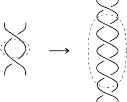
Since we obtain from by a region crossing change at any region in the two full twists and
Reidemeister moves of type II (see Figure 17),
we have .

Next, we prove by an indirect proof. We assume that . Let be the minimal crossing diagram of . Let be a set of regions of such that represents the trivial knot. Since the number of bigonal regions of is and , there exist connected four bigonal regions satisfying the following condition: One region of them is in , and the other three regions of them are not in . By applying a region crossing change at , we obtain from a diagram which represents the knot , and by applying Reidemeister moves of type II, we obtain from a minimal crossing diagram of . By region crossing changes at the regions of which corresponds to the regions of , we obtain from a diagram representing the trivial knot. Hence which contradicts . Hence we have , and therefore . The -torus knot has the region unknotting number one, and we can prove similarly for -torus knots. ∎
From Proposition 4.8, we have the following corollary:
Corollary 4.9.
For an arbitrary non-negative integer , there exists a knot which satisfies .
Appendix
In this appendix, we explain how to obtain another minimal crossing diagram by a flyping from a minimal crossing diagram of a prime alternating knot. Then we show how to obtain all the minimal crossing diagrams of a prime alternating knot. In this appendix, a tangle is a portion of a knot diagram from which there emerge just four arcs pointing in the four compass directions NW, NE, SW, and SE. For a tangle , we denote by (resp. ) the result of rotation in a horizontal (resp. vertical) axis, and that of crossing changes at all the crossing points of as shown in Figure 18.

We denote by (resp. ) the tangle with one crossing (resp. no crossings) as shown in the left side (resp. right side) of Figure 19.

For two tangles and , we define the sum of and to be the result of the operation of Figure 20. We also denote by the sum of and . A tangle is a tangle sum if , where neither nor is the tangle .

Let be a knot diagram which includes a tangle or . Flyping is a local transformation on which replaces by , or by as shown in Figure 21.

W. Menasco and M. Thistlethwaite showed that Tait’s third conjecture is true, that is, we can change into by performing a finite number of flypings for any two reduced alternating diagrams and of an alternating knot [4]. Hence we can obtain all the minimal crossing diagrams of a prime alternating knot from a minimal crossing diagram of by flypings. Let be a minimal crossing diagram of a non-trivial knot, and a crossing point of . Let be a tangle in whose NW arc and SW arc meet at as shown in Figure 22.

Since can be considered as the tangle or ,
we can apply a flyping there.
We call such a flyping flyping at and .
A flyping on a knot diagram is trivial if we obtain or the (vertical, horizontal, or vertical and horizontal) mirror image of
from by the flyping.
When we can apply a non-trivial flyping at a crossing point and a tangle of a diagram , we say that admits
a non-trivial flyping at (and ).
Now we explain how to obtain all the tangles such that admits non-trivial flypings at a crossing point and for a knot diagram .
From a knot diagram on and a crossing point of , we obtain two tangles and
such that we obtain from (resp. ) by connecting the NW arc and the NE arc, and the SW arc and the SW arc
see Figure 23, where we remark that the tangle (resp. ) corresponds to .

We note that and are unique by regarding that is equivalent to on . We remark that a flyping at and or is trivial because it comes out just horizontal mirror image of . Hence if neither nor is a tangle sum, the diagram does not admit a non-trivial flyping at . When is a tangle sum of tangles and , we can apply a flyping at and . Remark that a flyping at and is equivalent to a flyping at and up to horizontal mirror image see Figure 24.

Then we shall consider flypings at and only . For , the flyping at and is trivial if or is the sum of some tangles as shown in Figure 25.

The flyping at and is also trivial if and satisfy and , or and (see Figure 26).

Then, to obtain all the minimal crossing diagrams on of a reduced alternating knot ,
we will consider all the flypings at all the crossing points and all the tangles such that
of a minimal crossing diagram of except the following three cases:
- i:
-
the tangle is not a tangle sum ,
- ii:
-
the tangle or is the sum of some tangles ,
- iii:
-
the tangles and satisfy and , or and .
In the following examples, we will find all the minimal crossing diagrams of some knots by the above procedure.
Example 4.10.
A -torus knot has only one minimal crossing diagram on : Let in Figure 27 be the minimal crossing diagram of a -torus knot . For every crossing point , we obtain the same tangles and as shown in Figure 27.

The tangle is a sum of two tangles and , where is half twists and is half twists . The tangle is not a tangle sum. Then and satisfy the cases (ii) and (i), respectively. therefore, we can not apply non-trivial flypings on .
Similarly, we have the following example:
Example 4.11.
A knot with Conway’s notation or has only one minimal crossing diagram on .
We show that the knot has only one minimal crossing diagram on :
Example 4.12.
For the minimal crossing diagram of the knot in Figure 28, we call each crossing point and as shown in the figure.

Neither , , , , , , nor is a tangle sum, and are the tangle sums which consist of a tangle and the tangle , and is the tangle sum of the two tangles with vertical twists and satisfying and . The tangles , , , and are always tangle sums such that or is the sum of tangles (see Figure 29). Hence admits no non-trivial flypings, and therefore has only one minimal crossing diagram on .

We next show that the knot has just two minimal crossing diagrams on :
Example 4.13.
For the minimal crossing diagram of in Figure 30, we call each crossing and as shown in the figure. Then admits non-trivial flypings only at and the tangle and at and , and we obtain another diagram in Figure 31 by the flyping at and and at and , respectively, where we denote by and the tangles in Figure 30.

The diagram with the crossing points and in Figure 31 admits non-trivial flypings only at and , and , and , and and as depicted in Figure 31, and we obtain the diagram in Figure 30 by flyping there, respectively. Hence has just two minimal crossing diagrams and on .

Acknowledgments
The author is grateful to Akio Kawauchi, Taizo Kanenobu, and the members of Friday Seminar on Knot Theory in Osaka City University who assisted her in helpful advice, valuable discussions and the tender encouragement. She especially thanks Kengo Kishimoto for giving her such an interesting question and valuable advice and discussions. She also thanks Kenneth C. Millett and Makoto Ozawa for helpful comments, advice and information. She is deeply grateful to Jessica E. Banks for her valuable comments and many helpful suggestions. She is also grateful to the referee for careful reading and helpful advice. She was supported by JSPS Research Fellowships for Young Scientists.
References
- [1] H. Aida: Unknotting operations of polygonal type, Tokyo J. Math., 15 (1992), 111–121.
- [2] J. H. Conway: An enumeration of knots and links, and some of their algebraic properties, Computational Problems in Abstract Algebra, Pergamon Press, New-York (1970), 329–358.
- [3] A. Kawauchi: A survey of knot theory, Birkhauser, (1996).
- [4] W. Menasco and M. Thistlethwaite: The classification of alternating links, Ann. of Math., 138 (1993), 113–171.
- [5] W. W. Menasco and M. B. Thistlethwaite: The Tait flyping conjecture, Bull. Amer. Math. Soc. 25 (1991), 403–412
- [6] H. Murakami: Some metrics on classical knots, Math. Ann., 270 (1985), 35–45.
- [7] Y. Nakanishi: Replacements in the Conway third identity, Tokyo J. Math., 14 (1991), 197–203.
- [8] D. Rolfsen: Knots and links, Publish or Perish, Inc. (1976).
