Alexander-Conway invariants of tanglesThanks: Partially supported by the ISF grant 1343/10
Abstract.
We consider an algebra of (classical or virtual) tangles over an ordered circuit operad and introduce Conway-type invariants of tangles which respect this algebraic structure. The resulting invariants contain both the coefficients of the Conway polynomial and the Milnor’s -invariants of string links as partial cases. The extension of the Conway polynomial to virtual tangles satisfies the usual Conway skein relation and its coefficients are GPV finite type invariants. As a by-product, we also obtain a simple representation of the braid group which gives the Conway polynomial as a certain twisted trace.
Key words and phrases:
tangles, virtual links, Gauss diagrams, Conway polynomial2010 Mathematics Subject Classification
57M25; 57M271. Introduction
The Alexander polynomial of a link in is one the most celebrated and well-studied link invariants. A number of different definitions and approaches to are known (see e.g. [21, 24]) and it is related to a variety of interesting objects and constructions. The Alexander polynomial has reappeared time and again in all major developments in knot theory of the last decades: quantum invariants, finite type invariants, and, lately, the theory of knot Floer homology (see e.g. [17]).
In its original form, is only defined up to multiplication by powers of . Its close relative, the Conway polynomial , is free of this indeterminacy. The Conway polynomial may be obtained from by a substitution and is completely determined by its normalization on the unknot and the Conway skein relation
for any triple , and of link diagrams, which look as shown in Figure 1 in a certain disk and coincide outside this disk.

The importance of the Conway skein relation was realized after the appearance of the Jones polynomial, and led to the discovery of the HOMFLY polynomial [7].
The Alexander-Conway polynomial reappeared in the theory of quantum invariants (where it turned out to be related to the quantum supergroup , and also to at roots of unity), and later in the theory of Vassiliev knot invariants, since all coefficients of are finite type invariants (see [2]), with being an invariant of degree .
Separate coefficients of the Conway polynomial also attracted a lot of attention, with coefficients of low degrees been extensively studied. E.g., for knots, is the Casson knot invariant. For 2-component links is the linking number of two components, and is the Sato-Levine invariant. For algebraically split 3-component links is Milnor’s triple linking number. More generally, the first non-vanishing coefficient of for -component links is a certain combination of linking numbers [8]; for algebraically split links the first non-vanishing coefficient is a certain combination of Milnor triple linking numbers [13, 14, 23]. Coefficients of a link are related to those of a knot obtained by “banding together” components of (see [13]).
After the development of the theory of virtual knots (see [11]), a number of attempts was made to extend the definition of the Alexander or the Conway polynomial to the virtual case using one of the original approaches for classical links. In particular, J. Sawollek [22] constructed a polynomial which, however, vanishes on classical links. One of the possible paths to pursue is that of the quantum invariants, or Fox differential calculus. This allows one to generalize the Alexander polynomial to (virtual or classical) tangles, but results in polynomials which are not invariant under the first Reidemeister move and do not satisfy the skein relation (e.g., a recent construction of Archibald and Bar-Natan [1]). We are unaware of any generalizations of the Alexander-Conway polynomial to virtual links or tangles, which would coincide with the original polynomial on classical links and satisfy the skein relation.
With this goal in mind, we follow the approach of Chmutov, Khouri and Rossi [3], who use a tautological state sum model of Jaeger [9] to deduce Gauss diagram formulas for the coefficients of . We extend and modify their construction to ordered tangles and provide a direct proof of the invariance under the Reidemeister moves. This enables us to extend the coefficients to the virtual case as well. The resulting invariants are of finite type in the GPV sense [5] (and thus change under Kauffman’s virtualization move [11]).
We consider ordered tangles as an algebra over an ordered circuit operad. Our Conway-type invariants of tangles respect this algebraic structure. This allows us to “break” any complicated tangle into elementary fragments, so all proofs and calculations may be done for elementary tangles. The resulting invariants contain the coefficients of the Conway polynomial of (long) links as a partial case. For string links we use a certain shifted ordering to obtain Milnor’s triple and quadruple linking numbers. We conjecture that all Milnor’s homotopy -invariants of string links may be obtained in this way. As a by-product, we also obtain a simple representation of the braid group, which gives the Conway polynomial as a certain twisted trace. Due to the Conway skein relation, this representation factors through the Hecke algebra.
The paper is organized in the following way. In Section 2 we review classical and virtual ordered tangles. Section 3 is dedicated to the ordered circuit operad and its relation to ordered tangles. In Section 4 we introduce Conway-type invariants of tangles and then discuss their properties in Section 5.
2. Preliminaries
2.1. Classical and virtual tangles
Let be the unit 3-dimensional ball in . An -tangle in is a collection of disjoint oriented intervals and some number of circles, properly embedded in in such a way, that the endpoints of each interval belong to the set , where are some prescribed points on the boundary of . For example, one may choose points on the great circle , say, for odd and for even .
Tangles are considered up to an oriented isotopy in , fixed on the boundary. We will call embedded intervals and circles the strings and the closed components of a tangle, respectively. We will always assume that the only singularities of the projection of a tangle to the -plane are transversal double points. Such a projection, enhanced by an indication of an over/underpass in each double point, is called a tangle diagram. For technical reasons we will also often fix a base point (distinct from the endpoints of strings) on the boundary circle of the diagram. See Figure 2a.

Tangles generalize many objects, commonly considered in knot theory. In particular, tangles which have no strings are usual links in . Tangles with one string and no closed components are long knots, see Figure 2b. Pure tangles without closed components are called string links. Here a tangle is pure, if the endpoints of -th string, are and . A particular example of a pure tangle is the unit tangle, with every pair and connected by an interval. Braids are tangles such that each tangle component intersects every plane , in at most one point.
Virtual tangles present a useful generalization of tangles in the framework of the virtual knot theory [11]. In addition to usual crossings of a tangle diagram, one considers a new – virtual – type of crossings. We will draw virtual crossings as double points without any indication of the over- or underpass, see Figure 2c. Virtual tangle diagrams are considered up to the classical Reidemeister moves (see Figure 3) together with an additional set of virtual moves, shown in Figure 4.


Throughout the paper we will assume that all strings and closed components are oriented. Also, further we will consider only tangles with at least one string. To obtain invariants of closed classical links, we will pick one of the components, cut it open, and consider the resulting tangle with one string. We will then argue that the result does not depend on the choice. All our constructions will work both for classical and for virtual tangles.
2.2. Ordered tangles
Let be a tangle with strings. Since we assume that all strings are oriented, we can distinguish two endpoints of a string: its input (or source), and its output (or target). Denote by and sets of inputs and outputs of all strings of , respectively. A tangle is ordered, if the set is numbered by a collection of integers, so that each input is numbered by , and each output is numbered by for some . See Figure 5.

Orderings by different sets of integers which are related by a monotone map will be considered equivalent. Note that closed components do not appear in the definition of an ordering. Thus ordered closed links are usual links with no additional data, and 1-string tangles (in particular, long knots) have a unique ordering. We will call an ordering of a tangle coherent, if for every a string with the input numbered by has its output ordered by , see Figure 5a. For pure tangles (in particular string links) the standard ordering, such that is labeled by , is coherent.
3. Circuit operad and tangles
3.1. Circuit diagrams
A circuit operad [1] is a modification of a planar tangles operad [10], adjusted for virtual tangles instead of classical tangles. It may be useful to look at Figure 6 for some examples of circuit diagrams before reading the formal definition below.

An -circuit diagram , , is the unit disk in with a (possibly empty) collection of disjoint subdisks in the interior of . The boundary of the disk is called the output of , and the union of boundaries of , is the input of . Each disk has an even number of distinct marked points on its boundary (with ). Each boundary circle , is based, i.e., equipped with a base point distinct from the marked points; we will denote it by . The set of all marked points is equipped with a matching, i.e., is split in disjoint pairs. A pair is called external, if at least one of its points lie on the output , and is internal otherwise. It is convenient to think about each pair as a simple path in the complement of the internal disks, connecting the corresponding marked points. These connections represent only the matching of marked points, but not the actual path. Actual paths, as well as their intersections, are irrelevant, so we will treat these intersections as virtual crossings. Circuit diagrams are considered up to orientation-preserving diffeomorphisms. If paths in a circuit diagram may be realized without intersections in , we recover planar tangle diagrams of [10].
Two circuit diagrams and with the appropriate number of boundary points may be composed into a new circuit diagram as follows. Isotope so that the output of , together with the set of marked points and the base point, coincides with the input of . Glue into the internal disk of (smoothing near the marked points so that the paths of and meet smoothly) and remove the common boundary. See Figure 7. This composition defines a structure of a colored operad on circuit diagrams.

Further we will consider ordered oriented circuits. A circuit diagram is oriented, if all paths connecting pairs of marked points are oriented. In other words, each matched pair of marked points is ordered: – the source and the target of , respectively. The number of inputs and outputs on each circle are required to be equal (and thus equal to ). See Figures 6, 7. Compositions of oriented tangles should respect orientations of the paths.
3.2. Ordered circuit diagrams
An oriented circuit is ordered, if the set of paths is ordered, i.e., the set of all pairs of matched marked points is ordered: . We assume that two following conditions hold. Firstly, points and should be on the output of . Secondly, both points , , should be on the boundary of the same disk of . See the rightmost picture of Figure 8.
An ordering of all external paths in is called an external ordering, and an ordering of all internal paths in is called an internal ordering of . Given a (complete) ordering of , its restriction to external and internal paths defines an external and an internal orderings of , respectively. Vice versa, given both an internal and an external ordering of , one may construct different complete orderings of as shuffles of these two partial orderings, see Figure 8.

To define a composition of ordered circuits and , we require the following compatibility of orderings. A circuit of length in a circuit diagram is a sequence of paths, such that both endpoints and lie on the output , while the rest of the endpoints in this sequence lie on the inputs . For example, an ordered circuit diagram in Figure 8 contains three circuits of lengths , , and , respectively. If a sequential pair and of marked points on are identified with a pair and of marked points on , then we require that and are endpoints of a circuit in . The ordering on is then induced from orderings on and .
3.3. Inserting tangles in circuit diagrams
Given an -circuit diagram with inputs and a -tuple of tangles , we may create a new tangle if the data on the boundaries match. Isotope an tangle to such a position, that its boundary circle coincides with the input circle of and the endpoints of strings in coincide with the marked points on (if and are oriented, we also require a match of orientations). Glue into the internal disk of along the boundary, removing common boundary circles and thinking about paths in the complement as a virtual tangle diagram. Doing this for all disks , we obtain a new virtual -tangle in the disk . See Figure 9.

Note that in order to define an ordering of the resulting tangle , we need to fix only an external orientation on ; ’s need not to be ordered. Moreover, if has a (complete) ordering, it induces an ordering on each tangle . Indeed, an ordering of defines a numbering of the set of all marked points, which induces an ordering of marked points on the boundary circle , and thus an ordering of . If all ’s and are ordered, for the composition to be defined we require that this induced ordering should coincide with that of . See Figure 9.
This operation gives to virtual tangles a structure of an algebra over the circuit operad, similar to the usual case of classical tangles as an algebra over the planar operad.
4. Invariants of ordered tangles
4.1. States of tangle diagrams
Let be an ordered tangle diagram. An -state of is a collection of crossings of . A state of defines a new tangle diagram , obtained from by smoothing all crossings of respecting the orientation, see Figure 10a. The smoothed diagram inherits an ordering from . We will say that the state is coherent, if contains no closed components and the ordering of is coherent (see Section 2.2), i.e. if both ends of each string numbered by and for some . Suppose that is coherent. As we follow along the first string of (starting from its input and ending in its output), then continue to the second string of in the same fashion, etc., we pass a neighborhood of each smoothed crossing twice. A (coherent) state is descending, if we enter this neighborhood first time on the (former) overpass of , and the second – on the underpass. See Figure 10b. The sign of is defined as the product of signs (local writhe numbers) of all crossings in .

Remark 4.1.
Property of coherency of a state depends on the ordering of a diagram . Given a state such that contains no closed components, there are orderings of (which differ by reorderings of the strings of ) for which is coherent. To estimate the number of orderings for which such a state is descending, construct a graph with vertices corresponding to components (both open and closed) of , with two vertices connected by an edge if contains a crossing between two corresponding components of . If the number of connected components of this graph is , there are at most orderings of for which may be descending. In particular, if the graph is connected, there is at most one ordering for which may be descending.
4.2. Conway-type invariants of ordered tangles
Denote by the set of all descending -states of a diagram . Define and by
In particular, if has no closed components and the ordering of is coherent (indeed, in this case the empty state is descending), and otherwise.
Example 4.2.
For a trivial tangle diagram which consists of one straight string, the only descending state is trivial, thus . Also, an addition of a kink to a string of a tangle does not change the value of (since the new crossing cannot enter a coherent state). In particular, for a diagram obtained from by an addition of a small kink, we have . If a tangle diagram is split – i.e., it can be subdivided into two non-empty non-intersecting parts – then there are no coherent (and thus no descending) states, thus .
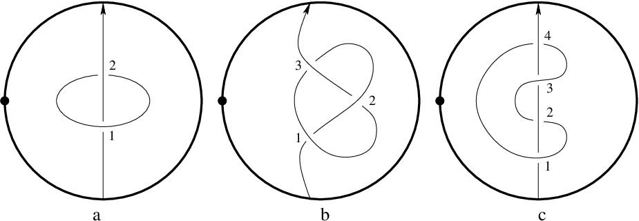
Example 4.3.
Let , , and be the diagrams shown in Figure 11. The only descending states for and are trivial, so . For there are no descending states, so . For there are two descending 1-states, but their signs are opposite, so .

Example 4.4.
For a diagram of a long Hopf link in Figure 12a there is only one descending state . Thus (depending on the orientation of the closed component). For the diagram of a long trefoil in Figure 12b there is only one non-trivial descending state , so . For the diagram of a long iterated Hopf link in Figure 12c, there are three non-trivial descending states: , and . Thus (depending on the orientation of the closed component).
Let be on oriented circuit diagram with an external ordering. Let ,…, be oriented tangles such that the composition is defined. Note that the external ordering of makes into an ordered tangle. Now, suppose that a (complete) ordering of extends the given external ordering. As discussed in Section 3.3, induces an ordering on each tangle ; denote the resulting ordered tangle by . Directly from the definition of we conclude that behaves multiplicatively under tangle compositions:
Lemma 4.5.
We have
where the summation is over all orderings of , extending the initial external ordering.
Theorem 4.6.
Let be a diagram of an ordered (classical or virtual) tangle . Then defines an invariant of ordered tangles.
Proof.
Let us prove the claim by checking the invariance of under the Reidemeister moves . The results of [19] imply that all oriented Reidemeister moves are generated by 4 moves shown in Figure 13 below.

Due to Lemma 4.5, it suffices to verify the claim only on pairs of elementary tangle diagrams of Figure 13 for different orderings. Indeed, a pair of ordered tangles which are related by an oriented Reidemeister move in a certain disk can be presented as compositions and with and being elementary tangle diagrams inside the disk , and being a tangle in a disk surrounding all other classical crossings, as illustrated in Figure 14.

If a pair of ordered diagrams differ by , the equality follows from Example 4.2. A similar equality for follows from Example 4.3.
Finally, if and are two ordered tangle diagrams related by , there is an obvious bijective correspondence between all descending 0- and 1-states of and ; also, there are no descending 3-states. This implies the required equality for every ordering for which there are no descending 2-states of and . But if for a certain ordering such states exist, they appear in pairs with opposite signs, and thus cancel out, see Figure 15.

∎
5. Properties of the invariants
5.1. Skein relation
Our choice of notation for the invariant of Theorem 4.6 is explained in the following proposition:
Proposition 5.1.
Let , and be ordered tangles which look as shown in Figure 16a inside a disk and coincide (including orderings) outside this disk. Then the Conway skein relation holds:

Proof.
The above proposition, together with the normalization of Example 4.2 on split tangles and on the trivial 1-string tangle, imply the following corollary:
Corollary 5.2 (c.f. [3]).
Let be a classical tangle with one string11 1 Recall that for a tangle with one string there is only one possible ordering. and closed components. Denote by a closed -component link, obtained from by the braid-type closure. Then is the Conway polynomial of .
5.2. Relation to Milnor’s -invariants
For invariants include well-known Milnor’s -invariants of link-homotopy [16] and their generalizations. In particular, let be a tangle with ordered strings and no closed components. Denote by the tangle equipped with an ordering which is obtained from the standard one by a cyclic permutation , i.e. such that the source and the target of the -th string are numbered by and , respectively, for , and the source and the target of the last string are numbered by and . See Figure 17. Denote .

The invariant detects Goussarov-Habiro’s move [4, 6]: an easy calculation shows that for tangles and depicted in Figure 17b we have , .
Conjecture 5.3.
Modulo lower degree invariants, coincide with Milnor’s link homotopy -invariant22 2 or rather, its generalization of [12] to (classical or virtual) tangles . In particular, if a closure is a Brunnian link, so that -th degree -invariants of are well-defined, we have .
Currently, the general structure of the lower degrees correction terms remains unclear. Here are some explicit formulas for low degree invariants, which directly follow from the results of [12, 18] (after a straightforward translation of formulas for and to the language of Gauss diagrams):
Proposition 5.4.
Let be a (possibly virtual) string link. Then
Cases when are no less interesting. Here are some results for small values of and . Denote by an invariant of 2-component string links introduced in [15], and let be the Casson knot invariant, i.e. the second coefficient of the Conway polynomial.
Proposition 5.5.
For a -string link with a standard ordering we have . This invariant is a splitting of the Casson knot invariant , in the following sense. For a long knot , denote by a -string link obtained from by a “reverse doubling”, i.e. by taking a pushed-off copy of along a zero framing, and then reversing its orientation. Then .
Proof.
The equality follows from equation 3.5 of [15]. Moreover, equation 2.2 of [15] implies that for any 2-string link with strings and one has , where is a plat closure of . Apply this equality to and note that the plat closure of is the unknot, thus . Also, is preserved under an orientation reversal, so . ∎
5.3. GPV finite type invariants
Finally, let us show that all invariants are finite type invariants of virtual tangles in the sense of GPV [5]. Recall, that for virtual links there are two different theories of finite type invariants. Kauffman’s theory of [11] is based on crossing changes similarly to the case of classical knots. GPV theory introduced in [5] is more restrictive in a sense that every GPV invariant is also a Kauffman invariant, but not vice versa. In GPV theory instead of crossing changes one uses a new operation, special for the virtual knot theory: crossing virtualization. Namely, given a real crossing in a diagram of a virtual link, we can convert it into a virtual crossing (resulting in a new virtual diagram).
Let be a virtual tangle diagram with marked and ordered real crossings , . Given an -tuple of zeros and ones, denote by a virtual tangle diagram obtained from by virtualization of all crossings with . Also, let . An invariant of virtual tangles is called a GPV finite type invariant of degree less than , if an alternating sum of its values on all diagrams vanishes:
for all diagrams and choices of crossings . If is of degree less than , but not less than , we say that is a GPV invariant of degree . A restriction to classical tangles of a GPV invariant of degree is a Vassiliev invariant of degree less than .
Remark 5.6.
An open (an highly non-trivial) conjecture is whether for long knots the opposite is true, i.e., whether any Vassiliev invariant of classical long knots can be extended to a GPV invariant. A positive solution would imply that Vassiliev invariants classify knots.
Proposition 5.7.
For any , the invariant is a GPV invariant of degree .
Proof.
In [5] it is shown that any invariant given by an arrow formula, where all arrow diagrams contain at most arrows, is a GPV invariant of degree at most . A straightforward translation of this statement into the language of state sums of Sections 4.1-4.2 implies that any invariant defined by a state sum, where the states contain at most crossings, is of degree at most . ∎
5.4. Conway-type representation of a braid group
If we restrict ourselves to braids instead of all -tangles, we can apply results of the previous section to obtain a following representation of the braid group on strands.
Let be polynomials in one variable with coefficients in the group ring of the symmetric group . Denote by and , the standard generators of and respectively.
Proposition 5.8.
For , define
Set and extend it to by linearity. This assignment defines an action of the braid group on . This representation satisfies , thus factors through the Hecke algebra.
Proof.
Use to order inputs of all strings on the top of an elementary tangle by . The only two orderings of the outputs of for which there exist a descending state are (for which the trivial state is descending) and (for which 1-state which consists of the only crossing of ) is descending. See Figure 18. This immediately leads to the expression for . The expression for is obtained in the same way. ∎

It would be interesting to identify this representation with (a quotient of) a known representation of the braid group.
The above representation may be used to recover the Conway polynomial as follows. For and , denote by the coefficient of in ; this defines a linear operator on . Composing it with a shift , , and taking the trace in , we define
Proposition 5.9.
Let be a link, obtained as a closure of a braid . Then is the coefficient of in the Conway-Alexander polynomial of .
Proof.
Follows from Corollary 5.2. ∎
References
- [1] J. Archibald, D. Bar-Natan, Circuit algebras and the Alexander polynomial for tangles, in preparation.
- [2] J. Birman, X.-S. Lin, Birman, Knot Polynomials and Vassiliev’s Invariants, Invent. Math. 111 (1993), 225–270.
- [3] S. Chmutov, M. Khoury, A. Rossi, Polyak-Viro formulas for coefficients of the Conway polynomial, J. Knot Theory and Ramif. 18 (2009), 773–783.
- [4] M. N. Goussarov, Variations of knotted graphs. The geometric technique of -equivalence (Russian), Algebra i Analiz 12 (2000) 79–125; engl. translation in St. Petersburg Math. J. 12 (2001) 569–604.
- [5] M. Goussarov, M. Polyak, O. Viro, Finite type invariants of virtual and classical knots, Topology 39 (2000), 1045–1068.
- [6] K. Habiro, Master’s thesis, University of Tokyo, 1994.
- [7] P. Freyd, D. Yetter, J. Hoste, W. B. R. Lickorish, K. Millett, A. Ocneanu, A new polynomial invariant of knots and links, Bull. AMS 12 (1985) 239–246.
- [8] J. Hoste, The first coefficient of the Conway polynomial, Proc. AMS, 95 (1985), 299302.
- [9] F. Jaeger, A combinatorial model for the HOMFLY polynomial, European J. Combinatorics 11 (1990), 549558.
- [10] V.F.R. Jones, Planar algebras I, New Zealand J. Math., to appear, arXiv.math.QA/9909027.
- [11] L. Kaufmann, Virtual knot theory, European J. Combin. 20 (1999), no. 7, 663–690.
- [12] O. Kravchenko M. Polyak, Milnor’s invariants and diassociative algebras, Lett. Math. Physics, to appear; preprint arxiv:1011.0117.
- [13] J. Levine, A factorization of the Conway polynomial, Comment. Math. Helv. 74 (1999), 2753.
- [14] G. Masbaum, A. Vaintrob, Milnor numbers, spanning trees, and the Alexander-Conway polynomial, Adv. Math, 180 (2003), 765–797.
- [15] J.-B. Meilhan, On Vassiliev invariants of order two for string links, J. Knot Theory and Ramif. 14 (2005), 665–687.
- [16] J. Milnor, Link groups, Annals of Math. 59 (1954), 177–195; Isotopy of links, Algebraic geometry and topology, A symposium in honor of S.Lefshetz, Princeton Univ. Press (1957).
- [17] P. Ozsvath, Z. Szabo, Holomorphic disks and knot invariants, Adv. Math, 186 (2004), 58–116.
- [18] M. Polyak, Skein relations for Milnor’s -invariants Alg. Geom. Topology 5 (2005), 1471–1479.
- [19] M. Polyak, Minimal generating sets of Reidemeister moves, Quantum Topology, 1 (2010), 399–411
- [20] M. Polyak, O. Viro, Gauss diagram formulas for Vassiliev invariants, Int. Math. Res. Notices 11 (1994), 445–454.
- [21] D. Rolfsen, Knots and Links (2nd ed.), Berkeley, CA: Publish or Perish (1990).
- [22] J. Sawollek, On Alexander-Conway polynomials for virtual knots and links, J. Knot Theory and Ramif. 12 (2002), 767–779.
- [23] L. Traldi, Conways potential function and its Taylor series, Kobe J.Math. 5 (1988), 233–264.
- [24] V. Turaev, Reidemeister torsion in knot theory, Russian Math. Surveys, 41:1 (1986), 119–182.