At the lowest order in the perturbation theory, the associated production of the vector gauge boson and the graviton takes place via the quark anti-quark initiated subprocess, given by

where $V=Z,W^{\pm}$ and $a,b$ are flavor indices. The corresponding Feynman diagrams are shown in Fig. (1). These diagrams are obtained by considering the tree level $q\bar{q}V$ diagram and by attaching the graviton line to all the possible external legs and the $q\bar{q}V$ vertex.

The Feynman rules and the summation of polarization tensor of the graviton are given in [3, 4]. The couplings of the fermions to the $Z$ and $W$ bosons are given by

where

and the coefficients $C_{v}$ and $C_{a}$ are

Here, $Q_{f}$ and $T_{3}^{f}$ denote the electric charge and the third component of the isospin of the quarks respectively, and $\theta_{W}$ is the weak mixing angle. For the vector gauge boson, the propagator in the unitary gauge $(\xi\rightarrow\infty)$ has been used throughout. This choice of the unitary gauge in the electro weak sector has the advantage of having vanishing goldstone and ghost contributions. The leading order matrix elements for the associated production of $Z$-boson and the graviton are computed using the algebraic manipulation program FORM [21] and are given by (in $n$-dimensions)

where $D=(s-m_{Z}^{2})$ and $s,t,u$ are the usual Mandelstam invariants. The over all bar in LHS of eq. (8) represents that the matrix elements have been averaged over the spins and the colors of the initial state particles and summed over those of the final state ones.

At the NLO in the perturbation theory, the cross sections receive ${\cal O}(\alpha_{s})$ contributions from real emission as well as virtual diagrams. The integration over the phase space of the real emission diagrams will give rise to infra-red (IR) (soft and collinear) divergences in the limit where the additional parton at NLO is either soft and/or collinear to the initial state partons. On the other hand, the integration over the loop momenta in the virtual diagrams will also give rise to infrared divergences, in addition to the ultraviolet (UV) divergences. In our calculation, we regulate all these divergences using dimensional regularization with $n=4+\epsilon$ being the number of space time dimensions. Completely anti-commuting $\gamma_{5}$ prescription [22] is used to handle $\gamma_{5}$ in $n$ dimensions. Here, it should be noted that as the gravitons couple to the energy momentum tensor of the SM fields, which is a conserved quantity, there won’t be any UV divergences coming from the loop diagrams.

There are several methods available in the literature to compute NLO QCD corrections. Standard methods based on fully analytical computation deal with the phase space and loop integrals in $n$-dimensions and give a finite ${\cal O}(\alpha_{s})$ contribution to the cross sections, after the real and the virtual contributions are added together and the initial state collinear singularities are absorbed into the bare parton distribution functions. However, these methods are not useful whenever the particles in the final state are subjected to either histogramming or experimental cuts or some isolation algorithms. In such cases, semi analytical methods like phase space slicing method or dipole subtraction method are extremely useful. In the present work, we have resorted to the former with two cut offs to compute the radiative corrections. In this method, the IR divergences appearing in the real diagrams can be handled in a convenient way by slicing the soft and collinear divergent regions from the full three body phase space. The advantage of this method is that the integration over the remaining phase space can be carried out in $4$-dimensions, rather than in $n$-dimensions, using standard Monte-Carlo techniques. In what follows, we give some of the details about the implementation of this phase space slicing method in our NLO computation.

In this section, we will present briefly how we have implemented various constraints imposed by the two cut off phase space slicing method and cuts on the phase space integrals for the $2\rightarrow 3$ subprocesses. We are interested in the following cross section:

We have implemented this phase space parameterization in our numerical code written in Fortran 77. We set $p_{i}=k_{i}$ ($i=3,4,5$) and $m_{3}=m_{V},m_{4}=m$ in our code. Here $m_{V}$ is mass of the gauge boson and $m$ is mass of the graviton. The phase space integrations as well as various convolutions in the two and three body contributions are done using VEGAS multi dimensional integration package. In what follows, we present the impact of our NLO corrections on various observables.

In this section, we present various kinematic distributions for the associate production of the graviton and the vector gauge boson to NLO in QCD at the LHC. The results are presented for proton-proton collision energy of $\sqrt{S}=14$ TeV. As discussed before, the inclusive cross section for the graviton production involves the summation of all possible graviton modes. This summation in the continuum limit leads to an integral over the graviton mass. The limits of this integral are set by the kinematics from $0$ to $\sqrt{s}-m_{V}$, where $\sqrt{s}$ is the parton center of mass energy and $m_{V}=m_{Z},m_{W}$. The masses of the gauge bosons and the weak mixing angle are given by [25]

The fine structure constant is taken to be $\alpha=1/128$. Throughout our study, we have used CTEQ6L1 and CTEQ6.6M parton density sets [26] for LO and NLO cross sections respectively. The strong coupling constant is calculated at two loop order in the $\overline{MS}$ scheme with $\alpha_{s}(m_{Z})=0.118$ ($\Lambda_{\rm{QCD}}=0.226$ GeV). We have also set the number of light flavors $n_{f}=5$. The following cuts are used for our numerical study,

For the 2-body process, the missing transverse momentum is same as that of the gauge boson. On the other hand, for the 3-body process, it need not be so due to the presence of an observable jet in the final state and hence it amounts purely to the graviton transverse momentum. The observable jet is defined as the one that satisfies the following conditions:

Whenever the jet does not satisfy the above conditions, the missing transverse momentum is approximated to be that of the gauge boson.

The LED model is an effective field theory valid below the UV cut-off scale $M_{s}$, which is expected to be of the order of a few TeV . At the LHC energies ($\sqrt{S}=14$ TeV), it is very well possible that the partonic center of mass energies can exceed this scale $M_{s}$ and lead to the signals that do not correspond to the compactified extra dimensions of the LED model. This necessitates the need to quantify the UV sensitivity of the theory and this issue was already addressed in [3], according to which the cross sections can be computed in two different ways, one with truncation where the cross sections are set to zero whenever the hard scale $Q$ involved in the problem exceeds $M_{s}$, and the other with un-truncation where there is no such constraint imposed on the cross sections. As pointed out in [3], if these two results converge then the predictions are valid and the model is viable, otherwise the un-truncated cross sections can dominate the truncated ones, implying the calculations are not under control. In our calculation, we choose the hard scale to be the invariant mass of the gauge boson and the graviton, $Q=M_{ZG}$, which at LO is the same as the center of mass energy of the partons $\sqrt{s}$. We will consider both truncated as well as un-truncated cases, however, most of our distributions are obtained with our default choice of truncation scheme.

Before proceeding to the kinematic distributions, we will do some consistency checks on the calculation. First, we check for the stability of the cross sections against the variation of the slicing parameters, $\delta_{s},\delta_{c}$. The sum of the 2-body and the 3-body contributions given in eqns. (17) and (18) is expected to be independent of the choice of these slicing parameters that are introduced in the intermediate stages of the calculation. In fig.(4), we show the dependency of the transverse momentum distribution $p_{T}^{Z}$ on the slicing parameter $\delta_{s}$ keeping the ratio of $\delta_{s}$ to $\delta_{c}$, fixed at a value of $100$. This distribution is obtained using the hard truncation scheme for a particular choice of the model parameters $M_{s}=3$ TeV and $\delta=4$. It can be seen from the fig.(4) that both the 2-body and the 3-body contributions vary with $\delta_{s}$ but their sum is fairly stable against the variation of $\delta_{s}$ over a wide range. This ensures the proper implementation of the slicing method in our NLO computation.

Another useful check on the computation is to reproduce the cross sections for the associated production of the photon and the graviton at the LHC [14]. In order to do this, we recalculated both real emission as well as virtual contributions for this process and the corresponding soft and collinear pieces. We found that the following replacements

1. 1.

   ${(C_{V}^{2}+C_{A}^{2})\over 4}\to Q_{f}^{2}$

2. 2.

   $m_{z}\to 0$

3. 3.

   $T_{z}\to e$

in the two body and three body real emission matrix elements of the $Z/W^{\pm}$ boson with Graviton production processes correctly reproduce the corresponding matrix elements for photon with Graviton production processes. Here, $Q_{f}$ is the charge of the fermion and $e$ is the electromagnetic coupling. Using our symbolic program, the analytical expression for virtual contributions for this process agrees with one given in the appendix of [14]. In addition, using these recalculated quantities, we reproduced all the numerical results in [14] after taking their choice of parameters, cuts etc. It is important to note that the NLO cross sections, or the K-factors, are subject to the choice of the event selection or more precisely the cuts on the particles in the final state. In our calculation, however, the gauge bosons being massive, we present our results according to the cuts given in eqns. (32 & 33).

In fig.(5), the total cross section for the associated production of $Z$-boson and the graviton is shown as a function of $P_{T}^{min}$, to NLO in QCD at the LHC. The cross sections are given for both the truncated as well as the un-truncated cases and with the choice of model parameters $M_{s}=3$ TeV and $d=2$. A similar plot is shown for $d=4$ in fig.(6). The K-factors are found to have a mild dependency on $P_{T}^{min}$, varying from $1.6$ to $1.4$. In fig.(7), we have shown the variation of the truncated as well as un-truncated total cross sections with respect to the scale $M_{s}$, for the case $d=2$. The difference between the truncated and the un-truncated cross sections is mainly due to the contributions coming from the region $Q>M_{s}$. However, with increasing $M_{s}$ the parton fluxes corresponding to $Q$ in this region rapidly fall down and hence the difference between the two cross sections decreases with increase in $M_{s}$. Such a behavior is evident from the figures. (7) and (8), for $d=2$ and $d=4$ respectively. The corresponding K-factors are also shown in fig. (9). In the rest of our calculation we choose $P_{T}^{min}=400$ GeV and $M_{s}=3$ TeV.

Next, we present LO and NLO transverse momentum distributions of the $Z$-boson ($P_{T}^{Z}$) in fig.(10) for $d=2,4,6$ and the corresponding missing transverse momentum distributions ($P_{T}^{miss}$) in the left panel of fig.(11) for $d=2,4$. The QCD corrections enhance both $P_{T}^{Z}$ and $P_{T}^{miss}$ distributions. Note that the shape of the $P_{T}^{Z}$ distribution remains unaffected while this is not the case for $P_{T}^{miss}$ distribution. Such a pattern can be understood from the definition of $P_{T}^{miss}$ mentioned before.

Next, we present the rapidity distributions of $Z$ bosons. The rapidity of massive gauge bosons is defined by

where $E$ and $p_{z}$ are the energy and the longitudinal momentum components of the gauge boson in the lab frame. In the right panel of fig.(11), we have plotted the rapidity distribution of the $Z$-boson both at LO and at NLO for two different choices of the factorization scale: $\mu_{F}=P_{T}^{Z}/2~~{\rm and}~~2P_{T}^{Z}$. This distribution is obtained by integrating over the transverse momentum of the $Z$-boson from $700$ GeV to $750$ GeV, for $d=4$. Note that the NLO corrections increase the cross section. As expected, the inclusion of order $a_{s}$ corrections reduces the dependence on the arbitrary factorization scale $\mu_{F}$. The percentage of uncertainty in the cross sections at the central rapidity region $Y=0$, due the variation of the scale from $\mu_{F}=P_{T}^{Z}/2$ to $\mu_{F}=2P_{T}^{Z}$, is 18.9 at LO and it gets reduced to 8.6 at NLO.

In this section we discuss the impact of NLO QCD corrections on the associated production of charged gauge bosons ($W^{\pm}$) and the graviton at the LHC. The matrix elements for the $W^{\pm}$ case are identical to those for the $Z$-boson case but for the masses of the gauge bosons and their couplings to the quarks as seen in eqn. (6). Further, in the case of charged gauge bosons, the parton fluxes will also be different from those of the neutral gauge boson. The parton fluxes for the quark anti-quark annihilation process in the case of $Z$-boson are of the form $q\bar{q}$ ($q={u,d,s,c,b}$), while they are of the form $u\bar{d}~(d\bar{u})$ for $W^{+}(W^{-})$. For $W$ boson production cross sections, we will consider the mixing of quarks among different quark generations, as allowed by the CKM-matrix elements $V_{ij}$, with $(i=u,c,t)$ and $(j=d,s,b)$. In view of this, in the above parton fluxes, $u$ and $d$ correspond to any $up$-type and $down$-type quarks respectively. The CKM matrix elements are given by [25]

Since all our calculations are done in the massless limit of the partons, we have not included the top quark contribution in our calculation and set all $V_{tj}$’s to zero.

Similar to the case of $Z$ boson, we will present the total cross sections as well as the differential distributions for the associated production of $W^{\pm}$ boson and a graviton. In fig.(12) and fig.(20), we have shown the stability of the transverse momentum distributions of $W^{-}$ and $W^{+}$ respectively, with the slicing parameter $\delta_{s}$. These distributions are obtained for the choice of $P_{T}^{W}=500$ GeV, keeping the ratio $\delta_{s}/\delta_{c}$ fixed at 100. It can be seen from the figures that the sum of the $2$-body and $3$-body contributions is fairly stable against the variation of the slicing parameters. This ensures the proper implementation of the slicing method in our numerical code, taking into account the appropriate parton fluxes for $W^{\pm}$. Next, we present the total cross sections as a function of $P_{T}^{min}$ as well as $M_{s}$. In fig.(13) and fig.(14), we show truncated as well as untruncated total cross sections for $W^{-}$ case, as a function of $P_{T}^{min}$, for $d=2$ and $d=4$ respectively. It can be seen from these figures that the QCD corrections have enhanced the leading order cross sections considerably, but there is no significant change in the shape of the cross sections. Similar plots are shown for $W^{+}$ in fig.(21) and fig.(22).

In fig.(15) and fig.(16), we show the total cross sections for $W^{-}$ as a function of $M_{s}$ for $d=2$ and $d=4$, respectively. A set of similar plots for $W^{+}$ are shown in fig.(23) and fig.(24). Note that, in each of the above, the cross sections for $W^{+}$ are somewhat higher than the corresponding ones for $W^{-}$. This difference in the total cross sections can be understood from the respective parton fluxes for $W^{-}$ and $W^{+}$ at the LHC. The corresponding K-factors are shown in fig.(17) for $W^{-}$ and in fig.(25) for $W^{+}$. For the choice of the parameters we have considered, the K-factors are found to vary from $1.7$ to $1.4$ in the case of $W^{-}$ while they range from $1.65$ to $1.05$ for $W^{+}$. Note that the K-factors for $W^{-}$ case are comparable but a little higher than those for $W^{+}$, which again can be accounted for the differences in the parton fluxes. The fact that the valence quark contributions are negligible and the parton fluxes at LO for $W^{+}$ are higher compared to those for $W^{-}$ explains the behavior the above factors.

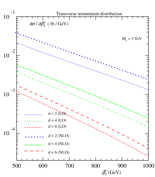
Further, in figs.(18) and (26), we present the transverse momentum distribution of $W^{-}$ and $W^{+}$ respectively as a function of the number of extra dimensions $d$ and for $M_{s}=3$ TeV. Similarly, we show the missing transverse momentum distribution the graviton when produced in association with $W^{-}$ in the left panel of fig.(19). In the right panel, we present the scale uncertainties in the rapidity distribution of $W^{-}$ by varying the factorization scale from $\mu_{F}=P_{T}^{W^{-}}/2$ to $\mu_{F}=2P_{T}^{W^{-}}$. This rapidity distribution is obtained by integrating over the transverse momentum $P_{T}^{W^{-}}$ from $700$ GeV to $750$ GeV. Similar plots are shown for $W^{+}$ in fig.(27). Note that the uncertainty resulting from the factorization scale $\mu_{F}$ get reduced as we include order $a_{s}$ corrections. The percentage of uncertainty at the central rapidity $Y^{W^{\pm}}=0$ is decreased from $19.1$ to $9.3$ in the case of $W^{-}$, whereas it gets reduced from $18.8$ to $8.3$ in the case of $W^{+}$.

References

• [1] N. Arkani-Hamed, S. Dimopoulos and G. Dvali, Phys. Lett. B 429 (1998) 263; I. Antoniadis, N. Arkani-Hamed, S. Dimopoulos and G. Dvali, Phys. Lett. B 436 (1998) 257; N. Arkani-Hamed, S. Dimopoulos and G. Dvali, Phys. Rev. D59 (1999) 086004.
• [2] D. J. Kapner et al. Phys. Rev. Lett. 98 (2007) 021101.
• [3] G. F. Giudice, R. Rattazzi, and J. D. Wells, Nucl. Phys. B544 (1999) 3.
• [4] T. Han, J. D. Lykken and R. J. Zhang, Phys. Rev. D59 (1999) 105006
• [5] P. Mathews, V. Ravindran and K. Sridhar, JHEP 0408 (2004) 048.
• [6] Prakash Mathews, V. Ravindran, K. Sridhar and W. L. van Neerven, Nucl. Phys. B713 (2005) 333; Prakash Mathews, V. Ravindran, K. Sridhar, JHEP 0510 (2005) 031; Prakash Mathews, V. Ravindran, Nucl. Phys. B753 (2006) 1; M.C. Kumar, Prakash Mathews, V. Ravindran, Eur. Phys. J. C49 (2007) 599.
• [7] E. A. Mirabelli, M. Perelstein and M. E. Peskin, Phys. Rev. Lett. 82 (1999) 2236.
• [8] Prakash Mathews, Sreerup Raychaudhuri, K. Sridhar, Phys. Lett. B450 (1999) 343; Phys. Lett. B455 (1999) 115; JHEP 0007 (2000) 008.
• [9] X. G. Wu and Z. Y. Fang, Phys. Rev. D78 (2008) 094002.
• [10] M.C. Kumar, Prakash Mathews, V. Ravindran, Anurag Tripathi, Phys. Lett. B672 (2009) 45; Nucl. Phys. B818 (2009) 28.
• [11] Neelima Agarwal, V. Ravindran, V. K. Tiwari, Anurag Tripathi, Nucl. Phys. B830 (2010) 248; Phys. Lett. B686 (2010) 244;
• [12] N. Agarwal, V. Ravindran, V. K. Tiwari and A. Tripathi, Phys. Lett. B 690 (2010) 390; Phys. Rev. D 82 (2010) 036001.
• [13] S. Karg, M. Karämer, Q. Li, D. Zeppenfeld, arXiv:0911.5095.
• [14] X Gao, C S Li, J Gao and J Wang, Phys. Rev. D81 (2010) 036008.
• [15] Kingman Cheung and Wai-Yee Keung, Phys. Rev. D60 (1999) 112003.
• [16] Gian F. Giudice, Tilman Plehn, Alessandro Strumia, Nucl. Phys. B706 (2005) 455.
• [17] Stefan Ask, Eur. Phys. J. C60 (2009) 509.
• [18] S. Ask, I.V. Akin, L. Benucci, A. De Roeck, M. Goebel, J. Haller, Comp. Phys. Comm. 181 (2010), 1593.
• [19] G. Aad et al. (ATLAS collaboration), CERN-OPEN-2008-020, arXiv:0901.0512v1[hep-ex].
• [20] M.C. Kumar, P. Mathews, V. Ravindran, S. Seth, arXiv:1004.5519 [hep-ph].
• [21] J. A. M. Vermaseren, math-ph/0010025.
• [22] M. Chanowitz, M. Furman and I. Hinchliffe, Nucl. Phys. B159 (1979) 225.
• [23] B.W. Harris, J.F. Owens, Phys. Rev. D 65 (2002) 094032.
• [24] G. Duplancic and B. Nizic, Eur. Phys. J. C 20 (2001) 357.
• [25] K. Nakamura et. al. Journal of Physics G 37, 075021 (2010).
• [26] P. M. Nadolsky et al., Phys. Rev. D 78 (2008) 013004
Appendix A
1 Finite part of the virtual contribution
All the ViV_{i}’s appearing in eqn. (16) are given below:
V1\displaystyle V_{1} =\displaystyle= 1(t2​u​(mz2−s))((−2m8t+2m6(mZ2(−6t+u)+t(7t+2u))−m4(18mZ4t\displaystyle{1\over(t^{2}u(m_{z}^{2}-s))}((-2m^{8}t+2m^{6}(m_{Z}^{2}(-6t+u)+t(7t+2u))-m^{4}(18m_{Z}^{4}t
OPEN−2​mZ2​(24​t2+6​t​u−u2)+3​t​(10​t2+8​t​u+u2))+m2​t​(−8​mZ6+26​t3+36​t2​uCLOSE\displaystyle-2m_{Z}^{2}(24t^{2}+6tu-u^{2})+3t(10t^{2}+8tu+u^{2}))+m^{2}t(-8m_{Z}^{6}+26t^{3}+36t^{2}u
OPEN+15​t​u2+u3+2​mZ4​(21​t+5​u)−2​mZ2​(30​t2+23​t​u+u2))−4​t2​(−2​mZ6+2​t3CLOSE\displaystyle+15tu^{2}+u^{3}+2m_{Z}^{4}(21t+5u)-2m_{Z}^{2}(30t^{2}+23tu+u^{2}))-4t^{2}(-2m_{Z}^{6}+2t^{3}
+4t2u+3tu2+u3+mZ4(6t+4u)−mZ2(6t2+8tu+3u2))))\displaystyle+4t^{2}u+3tu^{2}+u^{3}+m_{Z}^{4}(6t+4u)-m_{Z}^{2}(6t^{2}+8tu+3u^{2}))))
V2\displaystyle V_{2} =\displaystyle= 1(t2​u​(mZ2−s))(16(2m8t+2m6(mZ2(6t−u)−t(7t+2u))+m4(18mZ4t\displaystyle{1\over(t^{2}u(m_{Z}^{2}-s))}(16(2m^{8}t+2m^{6}(m_{Z}^{2}(6t-u)-t(7t+2u))+m^{4}(18m_{Z}^{4}t
OPEN−2​mZ2​(24​t2+6​t​u−u2)+3​t​(10​t2+8​t​u+u2))−m2​t​(−8​mZ6+26​t3+36​t2​uCLOSE\displaystyle-2m_{Z}^{2}(24t^{2}+6tu-u^{2})+3t(10t^{2}+8tu+u^{2}))-m^{2}t(-8m_{Z}^{6}+26t^{3}+36t^{2}u
OPEN+15​t​u2+u3+2​mZ4​(21​t+5​u)−2​mZ2​(30​t2+23​t​u+u2))+4​t2​(−2​mZ6+2​t3CLOSE\displaystyle+15tu^{2}+u^{3}+2m_{Z}^{4}(21t+5u)-2m_{Z}^{2}(30t^{2}+23tu+u^{2}))+4t^{2}(-2m_{Z}^{6}+2t^{3}
V3\displaystyle V_{3} =\displaystyle= V2|t↔u\displaystyle V_{2}|_{t\leftrightarrow u}
V4\displaystyle V_{4} =\displaystyle= V1|t↔u\displaystyle V_{1}|_{t\leftrightarrow u}
V5\displaystyle V_{5} =\displaystyle= 1(2​t2​u2​(−m2+t+u))​((4​m8​t​u−2​m6​(9​t​u​(t+u)+mZ2​(t2−12​t​u+u2))CLOSECLOSE\displaystyle{1\over(2t^{2}u^{2}(-m^{2}+t+u))}((4m^{8}tu-2m^{6}(9tu(t+u)+m_{Z}^{2}(t^{2}-12tu+u^{2}))
+m4​(36​mZ4​t​u+3​t​u​(11​t2+16​t​u+11​u2)+2​mZ2​(t3−30​t2​u−30​t​u2+u3))\displaystyle+m^{4}(36m_{Z}^{4}tu+3tu(11t^{2}+16tu+11u^{2})+2m_{Z}^{2}(t^{3}-30t^{2}u-30tu^{2}+u^{3}))
+4​t​u​(−2​mZ6​(t+u)+(t+u)2​(2​t2+t​u+2​u2)+mZ4​(6​t2+8​t​u+6​u2)CLOSE\displaystyle+4tu(-2m_{Z}^{6}(t+u)+(t+u)^{2}(2t^{2}+tu+2u^{2})+m_{Z}^{4}(6t^{2}+8tu+6u^{2})
OPEN−mZ2​(6​t3+11​t2​u+11​t​u2+6​u3))−m2​t​u​(−16​mZ6+52​mZ4​(t+u)CLOSE\displaystyle-m_{Z}^{2}(6t^{3}+11t^{2}u+11tu^{2}+6u^{3}))-m^{2}tu(-16m_{Z}^{6}+52m_{Z}^{4}(t+u)
−2mZ2(31t2+46tu+31u2)+3(9t3+17t2u+17tu2+9u3))))\displaystyle-2m_{Z}^{2}(31t^{2}+46tu+31u^{2})+3(9t^{3}+17t^{2}u+17tu^{2}+9u^{3}))))
V6\displaystyle V_{6} =\displaystyle= 1(2​t2​u2​(−m2+t+u))​((4​m8​t​u−2​m6​(9​t​u​(t+u)+mZ2​(t2−12​t​u+u2))CLOSECLOSE\displaystyle{1\over(2t^{2}u^{2}(-m^{2}+t+u))}((4m^{8}tu-2m^{6}(9tu(t+u)+m_{Z}^{2}(t^{2}-12tu+u^{2}))
V7\displaystyle V_{7} =\displaystyle= V6\displaystyle V_{6}
V8\displaystyle V_{8} =\displaystyle= 1((m2−t)2​(mZ2−t)2​t2​(m2−t−u)​u)​((m12​mZ2​t​(−3​mZ2+2​t)CLOSECLOSE\displaystyle{1\over((m^{2}-t)^{2}(m_{Z}^{2}-t)^{2}t^{2}(m^{2}-t-u)u)}((m^{12}m_{Z}^{2}t(-3m_{Z}^{2}+2t)
−3​m10​mZ2​(mZ4​(6​t−u)+t2​(6​t+u)−mZ2​t​(13​t+u))+m8​(−27​mZ8​tCLOSE\displaystyle-3m^{10}m_{Z}^{2}(m_{Z}^{4}(6t-u)+t^{2}(6t+u)-m_{Z}^{2}t(13t+u))+m^{8}(-27m_{Z}^{8}t
+12​t4​u+3​mZ6​(38​t2+5​t​u−u2)+mZ2​t2​(48​t2+11​t​u+3​u2)\displaystyle+12t^{4}u+3m_{Z}^{6}(38t^{2}+5tu-u^{2})+m_{Z}^{2}t^{2}(48t^{2}+11tu+3u^{2})
OPEN−mZ4​t​(138​t2+50​t​u+3​u2))−4​t5​u​(4​mZ6−2​mZ4​(5​t+4​u)CLOSE\displaystyle-m_{Z}^{4}t(138t^{2}+50tu+3u^{2}))-4t^{5}u(4m_{Z}^{6}-2m_{Z}^{4}(5t+4u)
OPEN−t⁡(2​t2+5​t​u+3​u2)+mZ2​(8​t2+13​t​u+4​u2))+m4​t2​(12​mZ10CLOSE\displaystyle-t(2t^{2}+5tu+3u^{2})+m_{Z}^{2}(8t^{2}+13tu+4u^{2}))+m^{4}t^{2}(12m_{Z}^{10}
−2​mZ8​(39​t+7​u)+mZ6​(160​t2+61​t​u+5​u2)+t2​u​(56​t2+69​t​u+12​u2)\displaystyle-2m_{Z}^{8}(39t+7u)+m_{Z}^{6}(160t^{2}+61tu+5u^{2})+t^{2}u(56t^{2}+69tu+12u^{2})
OPEN+mZ2​t​(34​t3−107​t2​u−99​t​u2−12​u3)−2​mZ4​(64​t3+t2​u−2​t​u2+3​u3))\displaystyle+m_{Z}^{2}t(34t^{3}-107t^{2}u-99tu^{2}-12u^{3})-2m_{Z}^{4}(64t^{3}+t^{2}u-2tu^{2}+3u^{3}))
+m6​t​(−12​mZ10−27​mZ6​t​(8​t+3​u)−6​t3​u​(7​t+4​u)+mZ8​(89​t+15​u)CLOSE\displaystyle+m^{6}t(-12m_{Z}^{10}-27m_{Z}^{6}t(8t+3u)-6t^{3}u(7t+4u)+m_{Z}^{8}(89t+15u)
OPEN+mZ2​t​(−58​t3+29​t2​u+16​t​u2−2​u3)+mZ4​(198​t3+94​t2​u+23​t​u2+3​u3))\displaystyle+m_{Z}^{2}t(-58t^{3}+29t^{2}u+16tu^{2}-2u^{3})+m_{Z}^{4}(198t^{3}+94t^{2}u+23tu^{2}+3u^{3}))
+m2​t3​(4​mZ8​(4​t−u)+4​mZ4​t​(8​t2−22​t​u−17​u2)+4​mZ6​(−10​t2+6​t​u+u2)CLOSE\displaystyle+m^{2}t^{3}(4m_{Z}^{8}(4t-u)+4m_{Z}^{4}t(8t^{2}-22tu-17u^{2})+4m_{Z}^{6}(-10t^{2}+6tu+u^{2})
−t2u(34t2+65tu+27u2)+2mZ2t(−4t3+51t2u+69tu2+18u3))))\displaystyle-t^{2}u(34t^{2}+65tu+27u^{2})+2m_{Z}^{2}t(-4t^{3}+51t^{2}u+69tu^{2}+18u^{3}))))
V9\displaystyle V_{9} =\displaystyle= V8|t↔u\displaystyle V_{8}|_{t\leftrightarrow u}
V10\displaystyle V_{10} =\displaystyle= −1(t​u​(−m2+t+u)​(−4​m2​mZ2+(t+u)2)2)​(16​(104​m12​mZ4​(t+u)CLOSECLOSE\displaystyle-{1\over(tu(-m^{2}+t+u)(-4m^{2}m_{Z}^{2}+(t+u)^{2})^{2})}(16(104m^{12}m_{Z}^{4}(t+u)
+4​m10​mZ2​(96​mZ4​(t+u)−2​mZ2​(73​t2+74​t​u+73​u2)−3​(t3+13​t2​uCLOSECLOSE\displaystyle+4m^{10}m_{Z}^{2}(96m_{Z}^{4}(t+u)-2m_{Z}^{2}(73t^{2}+74tu+73u^{2})-3(t^{3}+13t^{2}u
OPENOPEN+13​t​u2+u3))+4​(t+u)5​(−2​mZ6​(t+u)+(t+u)2​(2​t2+t​u+2​u2)CLOSE\displaystyle+13tu^{2}+u^{3}))+4(t+u)^{5}(-2m_{Z}^{6}(t+u)+(t+u)^{2}(2t^{2}+tu+2u^{2})
OPEN+mZ4​(6​t2+8​t​u+6​u2)−mZ2​(6​t3+11​t2​u+11​t​u2+6​u3))\displaystyle+m_{Z}^{4}(6t^{2}+8tu+6u^{2})-m_{Z}^{2}(6t^{3}+11t^{2}u+11tu^{2}+6u^{3}))
+m4​(3​(t+u)5​(11​t2+16​t​u+11​u2)−16​mZ10​(17​t2+10​t​u+17​u2)CLOSE\displaystyle+m^{4}(3(t+u)^{5}(11t^{2}+16tu+11u^{2})-16m_{Z}^{10}(17t^{2}+10tu+17u^{2})
−8​mZ4​(t+u)3​(25​t2+132​t​u+25​u2)−12​mZ6​(t+u)2​(43​t2−108​t​u+43​u2)\displaystyle-8m_{Z}^{4}(t+u)^{3}(25t^{2}+132tu+25u^{2})-12m_{Z}^{6}(t+u)^{2}(43t^{2}-108tu+43u^{2})
OPEN+4​mZ2​(t+u)4​(49​t2+40​t​u+49​u2)+48​mZ8​(16​t3+11​t2​u+11​t​u2+16​u3))\displaystyle+4m_{Z}^{2}(t+u)^{4}(49t^{2}+40tu+49u^{2})+48m_{Z}^{8}(16t^{3}+11t^{2}u+11tu^{2}+16u^{3}))
−m2​(t+u)2​(−16​mZ8​(4​t2+11​t​u+4​u2)+2​mZ2​(t+u)3​(9​t2−26​t​u+9​u2)CLOSE\displaystyle-m^{2}(t+u)^{2}(-16m_{Z}^{8}(4t^{2}+11tu+4u^{2})+2m_{Z}^{2}(t+u)^{3}(9t^{2}-26tu+9u^{2})
+3​(t+u)4​(9​t2+8​t​u+9​u2)−4​mZ4​(t+u)2​(45​t2+26​t​u+45​u2)\displaystyle+3(t+u)^{4}(9t^{2}+8tu+9u^{2})-4m_{Z}^{4}(t+u)^{2}(45t^{2}+26tu+45u^{2})
OPEN+8​mZ6​(25​t3+64​t2​u+64​t​u2+25​u3))+4​m8​(146​mZ8​(t+u)+(t+u)5CLOSE\displaystyle+8m_{Z}^{6}(25t^{3}+64t^{2}u+64tu^{2}+25u^{3}))+4m^{8}(146m_{Z}^{8}(t+u)+(t+u)^{5}
+26​mZ2​(t+u)2​(t2+5​t​u+u2)−24​mZ6​(17​t2+16​t​u+17​u2)\displaystyle+26m_{Z}^{2}(t+u)^{2}(t^{2}+5tu+u^{2})-24m_{Z}^{6}(17t^{2}+16tu+17u^{2})
OPEN+4​mZ4​(69​t3+59​t2​u+59​t​u2+69​u3))+2​m6​(136​mZ10​(t+u)−9​(t+u)6CLOSE\displaystyle+4m_{Z}^{4}(69t^{3}+59t^{2}u+59tu^{2}+69u^{3}))+2m^{6}(136m_{Z}^{10}(t+u)-9(t+u)^{6}
−12​mZ8​(59​t2+54​t​u+59​u2)−mZ2​(t+u)3​(123​t2+286​t​u+123​u2)\displaystyle-12m_{Z}^{8}(59t^{2}+54tu+59u^{2})-m_{Z}^{2}(t+u)^{3}(123t^{2}+286tu+123u^{2})
−2​mZ4​(t+u)2​(157​t2−374​t​u+157​u2)+mZ6​(986​t3+866​t2​uCLOSE\displaystyle-2m_{Z}^{4}(t+u)^{2}(157t^{2}-374tu+157u^{2})+m_{Z}^{6}(986t^{3}+866t^{2}u
+866tu2+986u3)))π2)\displaystyle+866tu^{2}+986u^{3})))\pi^{2})
V11\displaystyle V_{11} =\displaystyle= −1(t2​u2​(−m2+t+u)​(−4​m2​mZ2+(t+u)2)2)​((−96​m12​mZ4​t​uCLOSECLOSE\displaystyle-{1\over(t^{2}u^{2}(-m^{2}+t+u)(-4m^{2}m_{Z}^{2}+(t+u)^{2})^{2})}((-96m^{12}m_{Z}^{4}tu
−4​t2​u2​(t+u)3​(−6​mZ6+16​mZ4​(t+u)−15​mZ2​(t+u)2+5​(t+u)3)\displaystyle-4t^{2}u^{2}(t+u)^{3}(-6m_{Z}^{6}+16m_{Z}^{4}(t+u)-15m_{Z}^{2}(t+u)^{2}+5(t+u)^{3})
+4​m10​mZ2​(120​mZ2​t​u​(t+u)+t​u​(−3​t2+34​t​u−3​u2)+12​mZ4​(t2CLOSECLOSE\displaystyle+4m^{10}m_{Z}^{2}(120m_{Z}^{2}tu(t+u)+tu(-3t^{2}+34tu-3u^{2})+12m_{Z}^{4}(t^{2}
OPENOPEN−12​t​u+u2))+m2​t​u​(2​mZ2​(t+u)4​(t2+18​t​u+u2)+(t+u)5​(3​t2CLOSECLOSE\displaystyle-12tu+u^{2}))+m^{2}tu(2m_{Z}^{2}(t+u)^{4}(t^{2}+18tu+u^{2})+(t+u)^{5}(3t^{2}
OPEN+64​t​u+3​u2)+2​mZ4​(t+u)3​(9​t2−272​t​u+9​u2)−4​mZ6​(t+u)2​(11​t2CLOSE\displaystyle+64tu+3u^{2})+2m_{Z}^{4}(t+u)^{3}(9t^{2}-272tu+9u^{2})-4m_{Z}^{6}(t+u)^{2}(11t^{2}
OPENOPEN−196​t​u+11​u2)+24​mZ8​(t3−13​t2​u−13​t​u2+u3))+m4​(192​mZ10​t​u​(t+u)CLOSE\displaystyle-196tu+11u^{2})+24m_{Z}^{8}(t^{3}-13t^{2}u-13tu^{2}+u^{3}))+m^{4}(192m_{Z}^{10}tu(t+u)
−9​t​u​(t+u)4​(t2+8​t​u+u2)−8​mZ8​t​u​(71​t2+30​t​u+71​u2)\displaystyle-9tu(t+u)^{4}(t^{2}+8tu+u^{2})-8m_{Z}^{8}tu(71t^{2}+30tu+71u^{2})
−2​mZ4​t​u​(t+u)2​(167​t2−1060​t​u+167​u2)+4​mZ6​t​u​(167​t3−227​t2​uCLOSE\displaystyle-2m_{Z}^{4}tu(t+u)^{2}(167t^{2}-1060tu+167u^{2})+4m_{Z}^{6}tu(167t^{3}-227t^{2}u
OPENOPEN−227​t​u2+167​u3)−mZ2​(t+u)3​(3​t4−20​t3​u+674​t2​u2−20​t​u3+3​u4))\displaystyle-227tu^{2}+167u^{3})-m_{Z}^{2}(t+u)^{3}(3t^{4}-20t^{3}u+674t^{2}u^{2}-20tu^{3}+3u^{4}))
−2​m8​(432​mZ8​t​u+t​u​(t+u)2​(3​t2−4​t​u+3​u2)+2​mZ2​t​u​(−15​t3+179​t2​uCLOSECLOSE\displaystyle-2m^{8}(432m_{Z}^{8}tu+tu(t+u)^{2}(3t^{2}-4tu+3u^{2})+2m_{Z}^{2}tu(-15t^{3}+179t^{2}u
OPEN+179​t​u2−15​u3)+8​mZ6​(3​t3−97​t2​u−97​t​u2+3​u3)+4​mZ4​(3​t4+118​t3​uCLOSE\displaystyle+179tu^{2}-15u^{3})+8m_{Z}^{6}(3t^{3}-97t^{2}u-97tu^{2}+3u^{3})+4m_{Z}^{4}(3t^{4}+118t^{3}u
OPENOPEN+66​t2​u2+118​t​u3+3​u4))+m6​(−384​mZ10​t​u+1312​mZ8​t​u​(t+u)CLOSE\displaystyle+66t^{2}u^{2}+118tu^{3}+3u^{4}))+m^{6}(-384m_{Z}^{10}tu+1312m_{Z}^{8}tu(t+u)
+4​t​u​(t+u)3​(3​t2+5​t​u+3​u2)−4​mZ6​t​u​(391​t2+294​t​u+391​u2)\displaystyle+4tu(t+u)^{3}(3t^{2}+5tu+3u^{2})-4m_{Z}^{6}tu(391t^{2}+294tu+391u^{2})
+mZ2​(t+u)2​(3​t4−70​t3​u+1230​t2​u2−70​t​u3+3​u4)+8​mZ4​(3​t5+111​t4​uCLOSE\displaystyle+m_{Z}^{2}(t+u)^{2}(3t^{4}-70t^{3}u+1230t^{2}u^{2}-70tu^{3}+3u^{4})+8m_{Z}^{4}(3t^{5}+111t^{4}u
−122t3u2−122t2u3+111tu4+3u5))))\displaystyle-122t^{3}u^{2}-122t^{2}u^{3}+111tu^{4}+3u^{5}))))
V12\displaystyle V_{12} =\displaystyle= 1(3​(m2−t)​t2​(−mZ2+t)​(m2−u)​u2​(−mZ2+u)​(mZ2−s)2​(4​m2​mZ2−(t+u)2))\displaystyle{1\over(3(m^{2}-t)t^{2}(-m_{Z}^{2}+t)(m^{2}-u)u^{2}(-m_{Z}^{2}+u)(m_{Z}^{2}-s)^{2}(4m^{2}m_{Z}^{2}-(t+u)^{2}))}
×((−12m16mZ2tu(22mZ4+20tu−21mZ2(t+u))+3m14(20t2u2(t+u)2\displaystyle\times((-12m^{16}m_{Z}^{2}tu(22m_{Z}^{4}+20tu-21m_{Z}^{2}(t+u))+3m^{14}(20t^{2}u^{2}(t+u)^{2}
+44​mZ8​(t2−12​t​u+u2)−10​mZ4​t​u​(29​t2+118​t​u+29​u2)+mZ6​(−44​t3CLOSE\displaystyle+44m_{Z}^{8}(t^{2}-12tu+u^{2})-10m_{Z}^{4}tu(29t^{2}+118tu+29u^{2})+m_{Z}^{6}(-44t^{3}
OPENOPEN+852​t2​u+852​t​u2−44​u3)−21​mZ2​t​u​(t3−13​t2​u−13​t​u2+u3))\displaystyle+852t^{2}u+852tu^{2}-44u^{3})-21m_{Z}^{2}tu(t^{3}-13t^{2}u-13tu^{2}+u^{3}))
+4​t3​u3​(t+u)2​(64​mZ10−176​mZ8​(t+u)+8​mZ6​(23​t2+49​t​u+23​u2)CLOSE\displaystyle+4t^{3}u^{3}(t+u)^{2}(64m_{Z}^{10}-176m_{Z}^{8}(t+u)+8m_{Z}^{6}(23t^{2}+49tu+23u^{2})
−3​t​u​(7​t3+5​t2​u+5​t​u2+7​u3)−6​mZ4​(16​t3+51​t2​u+51​t​u2+16​u3)\displaystyle-3tu(7t^{3}+5t^{2}u+5tu^{2}+7u^{3})-6m_{Z}^{4}(16t^{3}+51t^{2}u+51tu^{2}+16u^{3})
OPEN+mZ2​(24​t4+111​t3​u+134​t2​u2+111​t​u3+24​u4))−3​m12​(792​mZ10​t​uCLOSE\displaystyle+m_{Z}^{2}(24t^{4}+111t^{3}u+134t^{2}u^{2}+111tu^{3}+24u^{4}))-3m^{12}(792m_{Z}^{10}tu
+4​mZ8​(33​t3−601​t2​u−601​t​u2+33​u3)+t2​u2​(79​t3+257​t2​u+257​t​u2CLOSE\displaystyle+4m_{Z}^{8}(33t^{3}-601t^{2}u-601tu^{2}+33u^{3})+t^{2}u^{2}(79t^{3}+257t^{2}u+257tu^{2}
OPEN+79​u3)+mZ6​(−121​t4+2026​t3​u+5262​t2​u2+2026​t​u3−121​u4)\displaystyle+79u^{3})+m_{Z}^{6}(-121t^{4}+2026t^{3}u+5262t^{2}u^{2}+2026tu^{3}-121u^{4})
+mZ2​t​u​(−73​t4+142​t3​u+574​t2​u2+142​t​u3−73​u4)−mZ4​(11​t5CLOSE\displaystyle+m_{Z}^{2}tu(-73t^{4}+142t^{3}u+574t^{2}u^{2}+142tu^{3}-73u^{4})-m_{Z}^{4}(11t^{5}
OPENOPEN+326​t4​u+3015​t3​u2+3015​t2​u3+326​t​u4+11​u5))−3​m10​(352​mZ12​t​uCLOSE\displaystyle+326t^{4}u+3015t^{3}u^{2}+3015t^{2}u^{3}+326tu^{4}+11u^{5}))-3m^{10}(352m_{Z}^{12}tu
−2428​mZ10​t​u​(t+u)−t2​u2​(t+u)2​(127​t2+386​t​u+127​u2)\displaystyle-2428m_{Z}^{10}tu(t+u)-t^{2}u^{2}(t+u)^{2}(127t^{2}+386tu+127u^{2})
−22​mZ8​(6​t4−167​t3​u−430​t2​u2−167​t​u3+6​u4)+mZ6​(99​t5−1796​t4​uCLOSE\displaystyle-22m_{Z}^{8}(6t^{4}-167t^{3}u-430t^{2}u^{2}-167tu^{3}+6u^{4})+m_{Z}^{6}(99t^{5}-1796t^{4}u
OPEN−9887​t3​u2−9887​t2​u3−1796​t​u4+99​u5)+mZ2​t​u​(104​t5+521​t4​uCLOSE\displaystyle-9887t^{3}u^{2}-9887t^{2}u^{3}-1796tu^{4}+99u^{5})+m_{Z}^{2}tu(104t^{5}+521t^{4}u
OPEN+707​t3​u2+707​t2​u3+521​t​u4+104​u5)+mZ4​(33​t6+87​t5​u+2369​t4​u2CLOSE\displaystyle+707t^{3}u^{2}+707t^{2}u^{3}+521tu^{4}+104u^{5})+m_{Z}^{4}(33t^{6}+87t^{5}u+2369t^{4}u^{2}
OPENOPEN+6046​t3​u3+2369​t2​u4+87​t​u5+33​u6))+m8​(2112​mZ12​t​u​(t+u)CLOSE\displaystyle+6046t^{3}u^{3}+2369t^{2}u^{4}+87tu^{5}+33u^{6}))+m^{8}(2112m_{Z}^{12}tu(t+u)
−16​mZ10​t​u​(453​t2+1241​t​u+453​u2)+mZ8​(−132​t5+6321​t4​uCLOSE\displaystyle-16m_{Z}^{10}tu(453t^{2}+1241tu+453u^{2})+m_{Z}^{8}(-132t^{5}+6321t^{4}u
OPEN+36839​t3​u2+36839​t2​u3+6321​t​u4−132​u5)−3​t2​u2​(107​t5+809​t4​uCLOSE\displaystyle+36839t^{3}u^{2}+36839t^{2}u^{3}+6321tu^{4}-132u^{5})-3t^{2}u^{2}(107t^{5}+809t^{4}u
OPEN+1912​t3​u2+1912​t2​u3+809​t​u4+107​u5)+mZ6​(33​t6−1209​t5​uCLOSE\displaystyle+1912t^{3}u^{2}+1912t^{2}u^{3}+809tu^{4}+107u^{5})+m_{Z}^{6}(33t^{6}-1209t^{5}u
OPEN−20115​t4​u2−42434​t3​u3−20115​t2​u4−1209​t​u5+33​u6)+3​mZ2​t​u​(84​t6CLOSE\displaystyle-20115t^{4}u^{2}-42434t^{3}u^{3}-20115t^{2}u^{4}-1209tu^{5}+33u^{6})+3m_{Z}^{2}tu(84t^{6}
OPEN+943​t5​u+3098​t4​u2+4694​t3​u3+3098​t2​u4+943​t​u5+84​u6)+3​mZ4​(33​t7CLOSE\displaystyle+943t^{5}u+3098t^{4}u^{2}+4694t^{3}u^{3}+3098t^{2}u^{4}+943tu^{5}+84u^{6})+3m_{Z}^{4}(33t^{7}
OPENOPEN−77​t6​u−544​t5​u2+1792​t4​u3+1792​t3​u4−544​t2​u5−77​t​u6+33​u7))\displaystyle-77t^{6}u-544t^{5}u^{2}+1792t^{4}u^{3}+1792t^{3}u^{4}-544t^{2}u^{5}-77tu^{6}+33u^{7}))
+m2​t2​u2​(−1024​mZ12​t​u−mZ6​(t+u)3​(1033​t2+3430​t​u+1033​u2)CLOSE\displaystyle+m^{2}t^{2}u^{2}(-1024m_{Z}^{12}tu-m_{Z}^{6}(t+u)^{3}(1033t^{2}+3430tu+1033u^{2})
−32​mZ10​(14​t3−37​t2​u−37​t​u2+14​u3)+3​t​u​(t+u)2​(41​t4+170​t3​uCLOSE\displaystyle-32m_{Z}^{10}(14t^{3}-37t^{2}u-37tu^{2}+14u^{3})+3tu(t+u)^{2}(41t^{4}+170t^{3}u
OPEN+194​t2​u2+170​t​u3+41​u4)+8​mZ8​(142​t4+405​t3​u+478​t2​u2+405​t​u3CLOSE\displaystyle+194t^{2}u^{2}+170tu^{3}+41u^{4})+8m_{Z}^{8}(142t^{4}+405t^{3}u+478t^{2}u^{2}+405tu^{3}
OPEN+142​u4)+mZ4​(483​t6+4326​t5​u+13853​t4​u2+20660​t3​u3+13853​t2​u4CLOSE\displaystyle+142u^{4})+m_{Z}^{4}(483t^{6}+4326t^{5}u+13853t^{4}u^{2}+20660t^{3}u^{3}+13853t^{2}u^{4}
OPEN+4326​t​u5+483​u6)−2​mZ2​(69​t7+660​t6​u+2578​t5​u2+5301​t4​u3CLOSE\displaystyle+4326tu^{5}+483u^{6})-2m_{Z}^{2}(69t^{7}+660t^{6}u+2578t^{5}u^{2}+5301t^{4}u^{3}
OPENOPEN+5301​t3​u4+2578​t2​u5+660​t​u6+69​u7))+m6​(−32​mZ12​t​u​(33​t2CLOSECLOSE\displaystyle+5301t^{3}u^{4}+2578t^{2}u^{5}+660tu^{6}+69u^{7}))+m^{6}(-32m_{Z}^{12}tu(33t^{2}
OPEN+131​t​u+33​u2)+4​mZ10​t​u​(537​t3+4225​t2​u+4225​t​u2+537​u3)\displaystyle+131tu+33u^{2})+4m_{Z}^{10}tu(537t^{3}+4225t^{2}u+4225tu^{2}+537u^{3})
+3​t2​u2​(t+u)2​(49​t4+469​t3​u+862​t2​u2+469​t​u3+49​u4)−4​mZ8​t​u​(126​t4CLOSE\displaystyle+3t^{2}u^{2}(t+u)^{2}(49t^{4}+469t^{3}u+862t^{2}u^{2}+469tu^{3}+49u^{4})-4m_{Z}^{8}tu(126t^{4}
OPEN+4141​t3​u+9014​t2​u2+4141​t​u3+126​u4)+mZ6​(33​t7−630​t6​u+775​t5​u2CLOSE\displaystyle+4141t^{3}u+9014t^{2}u^{2}+4141tu^{3}+126u^{4})+m_{Z}^{6}(33t^{7}-630t^{6}u+775t^{5}u^{2}
OPEN+14222​t4​u3+14222​t3​u4+775​t2​u5−630​t​u6+33​u7)−3​mZ2​t​u​(43​t7CLOSE\displaystyle+14222t^{4}u^{3}+14222t^{3}u^{4}+775t^{2}u^{5}-630tu^{6}+33u^{7})-3m_{Z}^{2}tu(43t^{7}
OPEN+686​t6​u+3478​t5​u2+7861​t4​u3+7861​t3​u4+3478​t2​u5+686​t​u6+43​u7)\displaystyle+686t^{6}u+3478t^{5}u^{2}+7861t^{4}u^{3}+7861t^{3}u^{4}+3478t^{2}u^{5}+686tu^{6}+43u^{7})
+mZ4​(−33​t8+171​t7​u+5013​t6​u2+15053​t5​u3+18824​t4​u4+15053​t3​u5CLOSE\displaystyle+m_{Z}^{4}(-33t^{8}+171t^{7}u+5013t^{6}u^{2}+15053t^{5}u^{3}+18824t^{4}u^{4}+15053t^{3}u^{5}
OPENOPEN+5013​t2​u6+171​t​u7−33​u8))+m4​t​u​(2080​mZ12​t​u​(t+u)CLOSE\displaystyle+5013t^{2}u^{6}+171tu^{7}-33u^{8}))+m^{4}tu(2080m_{Z}^{12}tu(t+u)
−6​t​u​(t+u)3​(5​t4+96​t3​u+172​t2​u2+96​t​u3+5​u4)+8​mZ10​(24​t4CLOSE\displaystyle-6tu(t+u)^{3}(5t^{4}+96t^{3}u+172t^{2}u^{2}+96tu^{3}+5u^{4})+8m_{Z}^{10}(24t^{4}
OPEN−485​t3​u−1382​t2​u2−485​t​u3+24​u4)−mZ8​(423​t5+375​t4​u−8054​t3​u2CLOSE\displaystyle-485t^{3}u-1382t^{2}u^{2}-485tu^{3}+24u^{4})-m_{Z}^{8}(423t^{5}+375t^{4}u-8054t^{3}u^{2}
OPEN−8054​t2​u3+375​t​u4+423​u5)+mZ6​(237​t6+3942​t5​u+10563​t4​u2CLOSE\displaystyle-8054t^{2}u^{3}+375tu^{4}+423u^{5})+m_{Z}^{6}(237t^{6}+3942t^{5}u+10563t^{4}u^{2}
OPEN+11668​t3​u3+10563​t2​u4+3942​t​u5+237​u6)−mZ4​(39​t7+2514​t6​uCLOSE\displaystyle+11668t^{3}u^{3}+10563t^{2}u^{4}+3942tu^{5}+237u^{6})-m_{Z}^{4}(39t^{7}+2514t^{6}u
OPEN+14408​t5​u2+29959​t4​u3+29959​t3​u4+14408​t2​u5+2514​t​u6+39​u7)\displaystyle+14408t^{5}u^{2}+29959t^{4}u^{3}+29959t^{3}u^{4}+14408t^{2}u^{5}+2514tu^{6}+39u^{7})
+mZ2​(33​t8+777​t7​u+5388​t6​u2+16631​t5​u3+24742​t4​u4+16631​t3​u5CLOSE\displaystyle+m_{Z}^{2}(33t^{8}+777t^{7}u+5388t^{6}u^{2}+16631t^{5}u^{3}+24742t^{4}u^{4}+16631t^{3}u^{5}
+5388t2u6+777tu7+33u8))))\displaystyle+5388t^{2}u^{6}+777tu^{7}+33u^{8}))))
V13\displaystyle V_{13} =\displaystyle= 1((mZ2−t)2​t2​(mZ2−u)2​u2​(−m2+t+u)​(−4​m2​mZ2+(t+u)2)2)\displaystyle{1\over((m_{Z}^{2}-t)^{2}t^{2}(m_{Z}^{2}-u)^{2}u^{2}(-m^{2}+t+u)(-4m^{2}m_{Z}^{2}+(t+u)^{2})^{2})}
×(mZ2(−16m12mZ4tu(6mZ6−8mZ4(t+u)−2tu(t+u)+mZ2(3t2+8tu\displaystyle\times(m_{Z}^{2}(-16m^{12}m_{Z}^{4}tu(6m_{Z}^{6}-8m_{Z}^{4}(t+u)-2tu(t+u)+m_{Z}^{2}(3t^{2}+8tu
OPENOPEN+3​u2))+8​m10​mZ2​(6​mZ10​(t2−12​t​u+u2)+mZ8​(−12​t3+149​t2​u+149​t​u2CLOSECLOSE\displaystyle+3u^{2}))+8m^{10}m_{Z}^{2}(6m_{Z}^{10}(t^{2}-12tu+u^{2})+m_{Z}^{8}(-12t^{3}+149t^{2}u+149tu^{2}
OPEN−12​u3)+3​mZ4​t​u​(t3+45​t2​u+45​t​u2+u3)−t2​u2​(2​t3+t2​u+t​u2+2​u3)\displaystyle-12u^{3})+3m_{Z}^{4}tu(t^{3}+45t^{2}u+45tu^{2}+u^{3})-t^{2}u^{2}(2t^{3}+t^{2}u+tu^{2}+2u^{3})
+mZ2​t​u​(3​t4−2​t3​u−54​t2​u2−2​t​u3+3​u4)+mZ6​(6​t4−80​t3​u−284​t2​u2CLOSE\displaystyle+m_{Z}^{2}tu(3t^{4}-2t^{3}u-54t^{2}u^{2}-2tu^{3}+3u^{4})+m_{Z}^{6}(6t^{4}-80t^{3}u-284t^{2}u^{2}
OPENOPEN−80​t​u3+6​u4))+4​t2​u2​(t+u)3​(6​mZ12−28​mZ10​(t+u)+2​t​u​(t+u)2​(t2CLOSECLOSE\displaystyle-80tu^{3}+6u^{4}))+4t^{2}u^{2}(t+u)^{3}(6m_{Z}^{12}-28m_{Z}^{10}(t+u)+2tu(t+u)^{2}(t^{2}
OPEN+3​t​u+u2)+mZ8​(49​t2+110​t​u+49​u2)−mZ6​(41​t3+155​t2​u+155​t​u2CLOSE\displaystyle+3tu+u^{2})+m_{Z}^{8}(49t^{2}+110tu+49u^{2})-m_{Z}^{6}(41t^{3}+155t^{2}u+155tu^{2}
OPEN+41​u3)+mZ4​(17​t4+97​t3​u+166​t2​u2+97​t​u3+17​u4)−mZ2​(3​t5+26​t4​uCLOSE\displaystyle+41u^{3})+m_{Z}^{4}(17t^{4}+97t^{3}u+166t^{2}u^{2}+97tu^{3}+17u^{4})-m_{Z}^{2}(3t^{5}+26t^{4}u
OPENOPEN+71​t3​u2+71​t2​u3+26​t​u4+3​u5))−m8​(864​mZ14​t​u+24​mZ12​(2​t3−117​t2​uCLOSECLOSE\displaystyle+71t^{3}u^{2}+71t^{2}u^{3}+26tu^{4}+3u^{5}))-m^{8}(864m_{Z}^{14}tu+24m_{Z}^{12}(2t^{3}-117t^{2}u
OPEN−117​t​u2+2​u3)−4​mZ8​t​u​(293​t3+1581​t2​u+1581​t​u2+293​u3)\displaystyle-117tu^{2}+2u^{3})-4m_{Z}^{8}tu(293t^{3}+1581t^{2}u+1581tu^{2}+293u^{3})
+mZ10​(−72​t4+3012​t3​u+7672​t2​u2+3012​t​u3−72​u4)−2​t2​u2​(t5+15​t4​uCLOSE\displaystyle+m_{Z}^{10}(-72t^{4}+3012t^{3}u+7672t^{2}u^{2}+3012tu^{3}-72u^{4})-2t^{2}u^{2}(t^{5}+15t^{4}u
OPEN−20​t3​u2−20​t2​u3+15​t​u4+u5)−4​mZ4​t​u​(t5+19​t4​u−54​t3​u2CLOSE\displaystyle-20t^{3}u^{2}-20t^{2}u^{3}+15tu^{4}+u^{5})-4m_{Z}^{4}tu(t^{5}+19t^{4}u-54t^{3}u^{2}
OPEN−54​t2​u3+19​t​u4+u5)+mZ2​t​u​(3​t6+36​t5​u−23​t4​u2−688​t3​u3CLOSE\displaystyle-54t^{2}u^{3}+19tu^{4}+u^{5})+m_{Z}^{2}tu(3t^{6}+36t^{5}u-23t^{4}u^{2}-688t^{3}u^{3}
OPEN−23​t2​u4+36​t​u5+3​u6)+2​mZ6​(12​t6+57​t5​u+812​t4​u2+1470​t3​u3CLOSE\displaystyle-23t^{2}u^{4}+36tu^{5}+3u^{6})+2m_{Z}^{6}(12t^{6}+57t^{5}u+812t^{4}u^{2}+1470t^{3}u^{3}
OPENOPEN+812​t2​u4+57​t​u5+12​u6))−m2​t​u​(4​mZ12​(t+u)2​(23​t2−352​t​u+23​u2)CLOSE\displaystyle+812t^{2}u^{4}+57tu^{5}+12u^{6}))-m^{2}tu(4m_{Z}^{12}(t+u)^{2}(23t^{2}-352tu+23u^{2})
−24​mZ14​(t3−13​t2​u−13​t​u2+u3)+2​t​u​(t+u)4​(t4+13​t3​u+38​t2​u2CLOSE\displaystyle-24m_{Z}^{14}(t^{3}-13t^{2}u-13tu^{2}+u^{3})+2tu(t+u)^{4}(t^{4}+13t^{3}u+38t^{2}u^{2}
OPEN+13​t​u3+u4)+2​mZ8​(t+u)2​(59​t4−542​t3​u−2218​t2​u2−542​t​u3+59​u4)\displaystyle+13tu^{3}+u^{4})+2m_{Z}^{8}(t+u)^{2}(59t^{4}-542t^{3}u-2218t^{2}u^{2}-542tu^{3}+59u^{4})
−2​mZ10​(73​t5−845​t4​u−3284​t3​u2−3284​t2​u3−845​t​u4+73​u5)\displaystyle-2m_{Z}^{10}(73t^{5}-845t^{4}u-3284t^{3}u^{2}-3284t^{2}u^{3}-845tu^{4}+73u^{5})
−mZ2​(t+u)3​(3​t6+48​t5​u+237​t4​u2+236​t3​u3+237​t2​u4+48​t​u5+3​u6)\displaystyle-m_{Z}^{2}(t+u)^{3}(3t^{6}+48t^{5}u+237t^{4}u^{2}+236t^{3}u^{3}+237t^{2}u^{4}+48tu^{5}+3u^{6})
+2​mZ4​(t+u)2​(6​t6+87​t5​u+104​t4​u2−238​t3​u3+104​t2​u4+87​t​u5+6​u6)\displaystyle+2m_{Z}^{4}(t+u)^{2}(6t^{6}+87t^{5}u+104t^{4}u^{2}-238t^{3}u^{3}+104t^{2}u^{4}+87tu^{5}+6u^{6})
+mZ6​(−49​t7−73​t6​u+2017​t5​u2+6457​t4​u3+6457​t3​u4+2017​t2​u5CLOSE\displaystyle+m_{Z}^{6}(-49t^{7}-73t^{6}u+2017t^{5}u^{2}+6457t^{4}u^{3}+6457t^{3}u^{4}+2017t^{2}u^{5}
OPENOPEN−73​t​u6−49​u7))+m6​(−384​mZ16​t​u+1936​mZ14​t​u​(t+u)−4​mZ12​t​u​(859​t2CLOSECLOSE\displaystyle-73tu^{6}-49u^{7}))+m^{6}(-384m_{Z}^{16}tu+1936m_{Z}^{14}tu(t+u)-4m_{Z}^{12}tu(859t^{2}
OPEN+1806​t​u+859​u2)−t2​u2​(t+u)2​(3​t4+64​t3​u−130​t2​u2+64​t​u3+3​u4)\displaystyle+1806tu+859u^{2})-t^{2}u^{2}(t+u)^{2}(3t^{4}+64t^{3}u-130t^{2}u^{2}+64tu^{3}+3u^{4})
+8​mZ10​(3​t5+347​t4​u+1095​t3​u2+1095​t2​u3+347​t​u4+3​u5)−mZ8​(45​t6CLOSE\displaystyle+8m_{Z}^{10}(3t^{5}+347t^{4}u+1095t^{3}u^{2}+1095t^{2}u^{3}+347tu^{4}+3u^{5})-m_{Z}^{8}(45t^{6}
OPEN+1146​t5​u+3887​t4​u2+3460​t3​u3+3887​t2​u4+1146​t​u5+45​u6)+mZ2​t​u​(3​t7CLOSE\displaystyle+1146t^{5}u+3887t^{4}u^{2}+3460t^{3}u^{3}+3887t^{2}u^{4}+1146tu^{5}+45u^{6})+m_{Z}^{2}tu(3t^{7}
OPEN+115​t6​u+165​t5​u2−1811​t4​u3−1811​t3​u4+165​t2​u5+115​t​u6+3​u7)\displaystyle+115t^{6}u+165t^{5}u^{2}-1811t^{4}u^{3}-1811t^{3}u^{4}+165t^{2}u^{5}+115tu^{6}+3u^{7})
+2​mZ6​(9​t7+142​t6​u+348​t5​u2−1971​t4​u3−1971​t3​u4+348​t2​u5+142​t​u6CLOSE\displaystyle+2m_{Z}^{6}(9t^{7}+142t^{6}u+348t^{5}u^{2}-1971t^{4}u^{3}-1971t^{3}u^{4}+348t^{2}u^{5}+142tu^{6}
OPEN+9​u7)+mZ4​(3​t8−32​t7​u−340​t6​u2+2156​t5​u3+6490​t4​u4+2156​t3​u5CLOSE\displaystyle+9u^{7})+m_{Z}^{4}(3t^{8}-32t^{7}u-340t^{6}u^{2}+2156t^{5}u^{3}+6490t^{4}u^{4}+2156t^{3}u^{5}
OPENOPEN−340​t2​u6−32​t​u7+3​u8))+m4​(192​mZ16​t​u​(t+u)−8​mZ14​t​u​(101​t2CLOSECLOSE\displaystyle-340t^{2}u^{6}-32tu^{7}+3u^{8}))+m^{4}(192m_{Z}^{16}tu(t+u)-8m_{Z}^{14}tu(101t^{2}
OPEN+138​t​u+101​u2)+4​mZ12​t​u​(333​t3+379​t2​u+379​t​u2+333​u3)\displaystyle+138tu+101u^{2})+4m_{Z}^{12}tu(333t^{3}+379t^{2}u+379tu^{2}+333u^{3})
+2​mZ10​t​u​(−581​t4+30​t3​u+2118​t2​u2+30​t​u3−581​u4)+3​t2​u2​(t+u)3​(t4CLOSE\displaystyle+2m_{Z}^{10}tu(-581t^{4}+30t^{3}u+2118t^{2}u^{2}+30tu^{3}-581u^{4})+3t^{2}u^{2}(t+u)^{3}(t^{4}
OPEN+18​t3​u−2​t2​u2+18​t​u3+u4)−mZ2​t​u​(t+u)2​(3​t6+96​t5​u+209​t4​u2CLOSE\displaystyle+18t^{3}u-2t^{2}u^{2}+18tu^{3}+u^{4})-m_{Z}^{2}tu(t+u)^{2}(3t^{6}+96t^{5}u+209t^{4}u^{2}
OPEN−1132​t3​u3+209​t2​u4+96​t​u5+3​u6)−mZ8​(3​t7−613​t6​u+921​t5​u2CLOSE\displaystyle-1132t^{3}u^{3}+209t^{2}u^{4}+96tu^{5}+3u^{6})-m_{Z}^{8}(3t^{7}-613t^{6}u+921t^{5}u^{2}
OPEN+11961​t4​u3+11961​t3​u4+921​t2​u5−613​t​u6+3​u7)+mZ6​(6​t8−177​t7​uCLOSE\displaystyle+11961t^{4}u^{3}+11961t^{3}u^{4}+921t^{2}u^{5}-613tu^{6}+3u^{7})+m_{Z}^{6}(6t^{8}-177t^{7}u
OPEN+12​t6​u2+8745​t5​u3+18124​t4​u4+8745​t3​u5+12​t2​u6−177​t​u7+6​u8)\displaystyle+12t^{6}u^{2}+8745t^{5}u^{3}+18124t^{4}u^{4}+8745t^{3}u^{5}+12t^{2}u^{6}-177tu^{7}+6u^{8})
−mZ4​(3​t9−13​t8​u−338​t7​u2+1474​t6​u3+8410​t5​u4+8410​t4​u5CLOSE\displaystyle-m_{Z}^{4}(3t^{9}-13t^{8}u-338t^{7}u^{2}+1474t^{6}u^{3}+8410t^{5}u^{4}+8410t^{4}u^{5}
+1474t3u6−338t2u7−13tu8+3u9))))\displaystyle+1474t^{3}u^{6}-338t^{2}u^{7}-13tu^{8}+3u^{9}))))
V14\displaystyle V_{14} =\displaystyle= 1((m2−t)2​t2​(m2−u)2​(m2−t−u)​u2​(−4​m2​mZ2+(t+u)2)2)\displaystyle{1\over((m^{2}-t)^{2}t^{2}(m^{2}-u)^{2}(m^{2}-t-u)u^{2}(-4m^{2}m_{Z}^{2}+(t+u)^{2})^{2})}
(m2(96m18mZ4tu−4m16mZ2(158mZ2tu(t+u)+tu(−3t2+34tu−3u2)\displaystyle(m^{2}(96m^{18}m_{Z}^{4}tu-4m^{16}m_{Z}^{2}(158m_{Z}^{2}tu(t+u)+tu(-3t^{2}+34tu-3u^{2})
OPEN+12​mZ4​(t2−12​t​u+u2))−4​t3​u3​(t+u)2​(12​mZ6​t​u+6​t​u​(t+u)3CLOSE\displaystyle+12m_{Z}^{4}(t^{2}-12tu+u^{2}))-4t^{3}u^{3}(t+u)^{2}(12m_{Z}^{6}tu+6tu(t+u)^{3}
OPEN+mZ2​(t+u)2​(t2−11​t​u+u2)−mZ4​(t3+7​t2​u+7​t​u2+u3))\displaystyle+m_{Z}^{2}(t+u)^{2}(t^{2}-11tu+u^{2})-m_{Z}^{4}(t^{3}+7t^{2}u+7tu^{2}+u^{3}))
+2​m14​(432​mZ8​t​u+t​u​(t+u)2​(3​t2−4​t​u+3​u2)−4​mZ2​t​u​(8​t3−113​t2​uCLOSECLOSE\displaystyle+2m^{14}(432m_{Z}^{8}tu+tu(t+u)^{2}(3t^{2}-4tu+3u^{2})-4m_{Z}^{2}tu(8t^{3}-113t^{2}u
OPEN−113​t​u2+8​u3)+4​mZ6​(18​t3−281​t2​u−281​t​u2+18​u3)+2​mZ4​(6​t4CLOSE\displaystyle-113tu^{2}+8u^{3})+4m_{Z}^{6}(18t^{3}-281t^{2}u-281tu^{2}+18u^{3})+2m_{Z}^{4}(6t^{4}
OPENOPEN+411​t3​u+578​t2​u2+411​t​u3+6​u4))+m2​t2​u2​(48​mZ8​t​u​(3​t2−2​t​u+3​u2)CLOSE\displaystyle+411t^{3}u+578t^{2}u^{2}+411tu^{3}+6u^{4}))+m^{2}t^{2}u^{2}(48m_{Z}^{8}tu(3t^{2}-2tu+3u^{2})
+2​(t+u)4​(3​t4+29​t3​u+72​t2​u2+29​t​u3+3​u4)−mZ2​(t+u)3​(5​t4CLOSE\displaystyle+2(t+u)^{4}(3t^{4}+29t^{3}u+72t^{2}u^{2}+29tu^{3}+3u^{4})-m_{Z}^{2}(t+u)^{3}(5t^{4}
OPEN+124​t3​u−102​t2​u2+124​t​u3+5​u4)+2​mZ4​(t+u)2​(7​t4+86​t3​u−522​t2​u2CLOSE\displaystyle+124t^{3}u-102t^{2}u^{2}+124tu^{3}+5u^{4})+2m_{Z}^{4}(t+u)^{2}(7t^{4}+86t^{3}u-522t^{2}u^{2}
OPENOPEN+86​t​u3+7​u4)−4​mZ6​(3​t5+61​t4​u−164​t3​u2−164​t2​u3+61​t​u4+3​u5))\displaystyle+86tu^{3}+7u^{4})-4m_{Z}^{6}(3t^{5}+61t^{4}u-164t^{3}u^{2}-164t^{2}u^{3}+61tu^{4}+3u^{5}))
+m12​(384​mZ10​t​u−2288​mZ8​t​u​(t+u)−4​t​u​(t+u)3​(6​t2+t​u+6​u2)−CLOSE\displaystyle+m^{12}(384m_{Z}^{10}tu-2288m_{Z}^{8}tu(t+u)-4tu(t+u)^{3}(6t^{2}+tu+6u^{2})-
16​mZ6​(9​t4−207​t3​u−416​t2​u2−207​t​u3+9​u4)−8​mZ4​(9​t5+284​t4​uCLOSE\displaystyle 16m_{Z}^{6}(9t^{4}-207t^{3}u-416t^{2}u^{2}-207tu^{3}+9u^{4})-8m_{Z}^{4}(9t^{5}+284t^{4}u
OPEN+356​t3​u2+356​t2​u3+284​t​u4+9​u5)−mZ2​(3​t6−126​t5​u+2089​t4​u2CLOSE\displaystyle+356t^{3}u^{2}+356t^{2}u^{3}+284tu^{4}+9u^{5})-m_{Z}^{2}(3t^{6}-126t^{5}u+2089t^{4}u^{2}
OPENOPEN+4756​t3​u3+2089​t2​u4−126​t​u5+3​u6))+m10​(−576​mZ10​t​u​(t+u)CLOSE\displaystyle+4756t^{3}u^{3}+2089t^{2}u^{4}-126tu^{5}+3u^{6}))+m^{10}(-576m_{Z}^{10}tu(t+u)
+672​mZ8​t​u​(3​t2+7​t​u+3​u2)+t​u​(t+u)2​(39​t4+170​t3​u+222​t2​u2CLOSE\displaystyle+672m_{Z}^{8}tu(3t^{2}+7tu+3u^{2})+tu(t+u)^{2}(39t^{4}+170t^{3}u+222t^{2}u^{2}
OPEN+170​t​u3+39​u4)+16​mZ6​(3​t5−147​t4​u−424​t3​u2−424​t2​u3−147​t​u4CLOSE\displaystyle+170tu^{3}+39u^{4})+16m_{Z}^{6}(3t^{5}-147t^{4}u-424t^{3}u^{2}-424t^{2}u^{3}-147tu^{4}
OPEN+3​u5)+2​mZ4​(36​t6+915​t5​u+780​t4​u2−1286​t3​u3+780​t2​u4+915​t​u5CLOSE\displaystyle+3u^{5})+2m_{Z}^{4}(36t^{6}+915t^{5}u+780t^{4}u^{2}-1286t^{3}u^{3}+780t^{2}u^{4}+915tu^{5}
OPEN+36​u6)+mZ2​(9​t7−109​t6​u+2141​t5​u2+8903​t4​u3+8903​t3​u4+2141​t2​u5CLOSE\displaystyle+36u^{6})+m_{Z}^{2}(9t^{7}-109t^{6}u+2141t^{5}u^{2}+8903t^{4}u^{3}+8903t^{3}u^{4}+2141t^{2}u^{5}
OPENOPEN−109​t​u6+9​u7))−m4​t​u​(48​mZ8​t​u​(4​t3+3​t2​u+3​t​u2+4​u3)CLOSE\displaystyle-109tu^{6}+9u^{7}))-m^{4}tu(48m_{Z}^{8}tu(4t^{3}+3t^{2}u+3tu^{2}+4u^{3})
−mZ2​t​u​(t+u)2​(85​t4−52​t3​u−1286​t2​u2−52​t​u3+85​u4)+(t+u)3​(3​t6CLOSE\displaystyle-m_{Z}^{2}tu(t+u)^{2}(85t^{4}-52t^{3}u-1286t^{2}u^{2}-52tu^{3}+85u^{4})+(t+u)^{3}(3t^{6}
OPEN+58​t5​u+303​t4​u2+492​t3​u3+303​t2​u4+58​t​u5+3​u6)−4​mZ6​(3​t6CLOSE\displaystyle+58t^{5}u+303t^{4}u^{2}+492t^{3}u^{3}+303t^{2}u^{4}+58tu^{5}+3u^{6})-4m_{Z}^{6}(3t^{6}
OPEN+108​t5​u−55​t4​u2−608​t3​u3−55​t2​u4+108​t​u5+3​u6)+mZ4​(15​t7CLOSE\displaystyle+108t^{5}u-55t^{4}u^{2}-608t^{3}u^{3}-55t^{2}u^{4}+108tu^{5}+3u^{6})+m_{Z}^{4}(15t^{7}
OPENOPEN+353​t6​u−501​t5​u2−5475​t4​u3−5475​t3​u4−501​t2​u5+353​t​u6+15​u7))\displaystyle+353t^{6}u-501t^{5}u^{2}-5475t^{4}u^{3}-5475t^{3}u^{4}-501t^{2}u^{5}+353tu^{6}+15u^{7}))
+m8​(192​mZ10​t​u​(t2+4​t​u+u2)−32​mZ8​t​u​(20​t3+97​t2​u+97​t​u2+20​u3)CLOSE\displaystyle+m^{8}(192m_{Z}^{10}tu(t^{2}+4tu+u^{2})-32m_{Z}^{8}tu(20t^{3}+97t^{2}u+97tu^{2}+20u^{3})
−3​t​u​(t+u)3​(11​t4+80​t3​u+122​t2​u2+80​t​u3+11​u4)+32​mZ6​t​u​(27​t4CLOSE\displaystyle-3tu(t+u)^{3}(11t^{4}+80t^{3}u+122t^{2}u^{2}+80tu^{3}+11u^{4})+32m_{Z}^{6}tu(27t^{4}
OPEN+104​t3​u+77​t2​u2+104​t​u3+27​u4)−2​mZ4​(12​t7+423​t6​u+483​t5​u2CLOSE\displaystyle+104t^{3}u+77t^{2}u^{2}+104tu^{3}+27u^{4})-2m_{Z}^{4}(12t^{7}+423t^{6}u+483t^{5}u^{2}
OPEN−3970​t4​u3−3970​t3​u4+483​t2​u5+423​t​u6+12​u7)−mZ2​(9​t8−36​t7​uCLOSE\displaystyle-3970t^{4}u^{3}-3970t^{3}u^{4}+483t^{2}u^{5}+423tu^{6}+12u^{7})-m_{Z}^{2}(9t^{8}-36t^{7}u
OPENOPEN+880​t6​u2+7376​t5​u3+13062​t4​u4+7376​t3​u5+880​t2​u6−36​t​u7+9​u8))\displaystyle+880t^{6}u^{2}+7376t^{5}u^{3}+13062t^{4}u^{4}+7376t^{3}u^{5}+880t^{2}u^{6}-36tu^{7}+9u^{8}))
+m6​(−192​mZ10​t2​u2​(t+u)+16​mZ8​t​u​(3​t4+58​t3​u+62​t2​u2+58​t​u3CLOSECLOSE\displaystyle+m^{6}(-192m_{Z}^{10}t^{2}u^{2}(t+u)+16m_{Z}^{8}tu(3t^{4}+58t^{3}u+62t^{2}u^{2}+58tu^{3}
OPEN+3​u4)−4​mZ6​t​u​(41​t5+337​t4​u−308​t3​u2−308​t2​u3+337​t​u4+41​u5)\displaystyle+3u^{4})-4m_{Z}^{6}tu(41t^{5}+337t^{4}u-308t^{3}u^{2}-308t^{2}u^{3}+337tu^{4}+41u^{5})
+t​u​(t+u)2​(15​t6+194​t5​u+697​t4​u2+1016​t3​u3+697​t2​u4+194​t​u5CLOSE\displaystyle+tu(t+u)^{2}(15t^{6}+194t^{5}u+697t^{4}u^{2}+1016t^{3}u^{3}+697t^{2}u^{4}+194tu^{5}
OPEN+15​u6)+mZ4​t​u​(195​t6+916​t5​u−4815​t4​u2−12032​t3​u3−4815​t2​u4CLOSE\displaystyle+15u^{6})+m_{Z}^{4}tu(195t^{6}+916t^{5}u-4815t^{4}u^{2}-12032t^{3}u^{3}-4815t^{2}u^{4}
OPEN+916​t​u5+195​u6)+mZ2​(3​t9−t8​u−20​t7​u2+2332​t6​u3+7838​t5​u4CLOSE\displaystyle+916tu^{5}+195u^{6})+m_{Z}^{2}(3t^{9}-t^{8}u-20t^{7}u^{2}+2332t^{6}u^{3}+7838t^{5}u^{4}
+7838t4u5+2332t3u6−20t2u7−tu8+3u9))))\displaystyle+7838t^{4}u^{5}+2332t^{3}u^{6}-20t^{2}u^{7}-tu^{8}+3u^{9}))))
V15\displaystyle V_{15} =\displaystyle= 1(6​t2​u2​(−m2+t+u)2)((144m10tu−6m8(97tu(t+u)+12mZ2(t2−12tu\displaystyle{1\over(6t^{2}u^{2}(-m^{2}+t+u)^{2})}((144m^{10}tu-6m^{8}(97tu(t+u)+12m_{Z}^{2}(t^{2}-12tu (1)
OPENOPEN+u2))+3​m6​(432​mZ4​t​u+t​u​(353​t2+700​t​u+353​u2)+mZ2​(48​t3−746​t2​uCLOSECLOSE\displaystyle+u^{2}))+3m^{6}(432m_{Z}^{4}tu+tu(353t^{2}+700tu+353u^{2})+m_{Z}^{2}(48t^{3}-746t^{2}u
OPENOPEN−746​t​u2+48​u3))+12​m4​(48​mZ6​t​u−208​mZ4​t​u​(t+u)−t​u​(89​t3+249​t2​uCLOSECLOSE\displaystyle-746tu^{2}+48u^{3}))+12m^{4}(48m_{Z}^{6}tu-208m_{Z}^{4}tu(t+u)-tu(89t^{3}+249t^{2}u
OPENOPEN+249​t​u2+89​u3)+mZ2​(−6​t4+199​t3​u+482​t2​u2+199​t​u3−6​u4))\displaystyle+249tu^{2}+89u^{3})+m_{Z}^{2}(-6t^{4}+199t^{3}u+482t^{2}u^{2}+199tu^{3}-6u^{4}))
+m2​t​u​(−696​mZ6​(t+u)+40​mZ4​(39​t2+107​t​u+39​u2)−6​mZ2​(229​t3CLOSECLOSE\displaystyle+m^{2}tu(-696m_{Z}^{6}(t+u)+40m_{Z}^{4}(39t^{2}+107tu+39u^{2})-6m_{Z}^{2}(229t^{3}
OPENOPEN+817​t2​u+817​t​u2+229​u3)+21​(27​t4+98​t3​u+126​t2​u2+98​t​u3+27​u4))\displaystyle+817t^{2}u+817tu^{2}+229u^{3})+21(27t^{4}+98t^{3}u+126t^{2}u^{2}+98tu^{3}+27u^{4}))
−4​t​u​(−2​mZ6​(15​t2+86​t​u+15​u2)+mZ4​(90​t3+406​t2​u+406​t​u2+90​u3)CLOSE\displaystyle-4tu(-2m_{Z}^{6}(15t^{2}+86tu+15u^{2})+m_{Z}^{4}(90t^{3}+406t^{2}u+406tu^{2}+90u^{3})
−mZ2​(90​t4+381​t3​u+512​t2​u2+381​t​u3+90​u4)+3​(10​t5+49​t4​u+69​t3​u2CLOSE\displaystyle-m_{Z}^{2}(90t^{4}+381t^{3}u+512t^{2}u^{2}+381tu^{3}+90u^{4})+3(10t^{5}+49t^{4}u+69t^{3}u^{2}
+69t2u3+49tu4+10u5))))\displaystyle+69t^{2}u^{3}+49tu^{4}+10u^{5}))))
2 B0B_{0} Integrals
B0​(𝒫)=i(4​π)2​[−2ϵ+2−γE−f⁡(𝒫)]\displaystyle B_{0}\left({\cal{P}}\right)=\frac{i}{(4\pi)^{2}}\left[-\frac{2}{\epsilon}+2-\gamma_{E}-f\left({\cal{P}}\right)\right] (2)
where 𝒫∈{p3,p4,p5,k,q}{\cal{P}}\ \in\ \{p_{3},p_{4},p_{5},k,q\}, kk is the momentum of vector boson, qq, the momentum of graviton, p3=p1+k,p4=p2+k,p5=p1+p2p_{3}=p_{1}+k,p_{4}=p_{2}+k,p_{5}=p_{1}+p_{2} and,
f⁡(𝒫)={ln⁡(−𝒫24​π​μr2)for𝒫=p3,p4ln⁡(𝒫24​π​μr2)−i​πfor𝒫=p5,k,q\displaystyle f\left({\cal{P}}\right)=\left\{\begin{array}[]{ll}\ln\left(\frac{-{\cal{P}}^{2}}{4\pi\mu_{r}^{2}}\right)&\mbox{for}\ \ {\cal{P}}=p_{3},p_{4}\\ \ln\left(\frac{{\cal{P}}^{2}}{4\pi\mu_{r}^{2}}\right)-i\pi&\mbox{for}\ \ {\cal{P}}=p_{5},k,q\\ \end{array}\right.
3 C0C_{0} Integrals
C0​(𝒫′,𝒫′′)=\displaystyle C_{0}\left({\cal{P^{\prime}}},{\cal{P^{\prime\prime}}}\right)=\!\!\!\!\!\!\!\!\!\! −i(4​π)21[(𝒫′−𝒫′′)2−𝒫′′2][−2ϵ{ln(−(𝒫′−𝒫′′)2𝒫′′2)+iπ}+\displaystyle\frac{-i}{(4\pi)^{2}}\ \frac{1}{[({\cal{P^{\prime}}}-{\cal{P^{\prime\prime}}})^{2}-{\cal{P^{\prime\prime}}}^{2}]}\left[-\frac{2}{\epsilon}{\left\{\ln\left(\frac{-({\cal{P^{\prime}}}-{\cal{P^{\prime\prime}}})^{2}}{{\cal{P^{\prime\prime}}}^{2}}\right)+i\pi\right\}}\ +\ \right. (6)
12{(γE+ln(𝒫′′24​π​μr2)−iπ)2−(γE+ln(−(𝒫′−𝒫′′)24​π​μr2))2}]\displaystyle\left.\frac{1}{2}\left\{{\left(\gamma_{E}+\ln\left(\frac{{\cal{P^{\prime\prime}}}^{2}}{4\pi\mu_{r}^{2}}\right)-i\pi\right)^{2}-{\left(\gamma_{E}+\ln\left(\frac{-({\cal{P^{\prime}}}-{\cal{P^{\prime\prime}}})^{2}}{4\pi\mu_{r}^{2}}\right)\right)}^{2}}\right\}\right]
where 𝒫′∈{p1,p2}{\cal{P}^{\prime}}\ \in\ \{p_{1},p_{2}\} and, 𝒫′′∈{k,q}{\cal{P}^{\prime\prime}}\ \in\ \{k,q\}
C0​(p1,p2)=\displaystyle C_{0}\left(p_{1},p_{2}\right)=\!\!\!\!\!\!\!\!\!\! −i(4​π)21s[−4ϵ2−2ϵ{γE+ln(s4​π​μr2)−iπ}+\displaystyle\frac{-i}{(4\pi)^{2}}\ \frac{1}{s}\left[-\frac{4}{\epsilon^{2}}-\frac{2}{\epsilon}{\left\{\gamma_{E}+\ln\left(\frac{s}{4\pi\mu_{r}^{2}}\right)-i\pi\right\}}\ +\ \right. (7)
12{π26−(γE+ln(s4​π​μr2)−iπ)2}]\displaystyle\left.\frac{1}{2}\left\{{\frac{\pi^{2}}{6}-{\left(\gamma_{E}+\ln\left(\frac{s}{4\pi\mu_{r}^{2}}\right)-i\pi\right)}^{2}}\right\}\right]
C0​(k,q)=\displaystyle\!\!\!\!\!\!\!\!C_{0}\left(k,q\right)=\!\!\!\!\!\!\!\!\!\! −i(4​π)21s​β[2Li2(21−α+β)−2Li2(21−α−β)−\displaystyle\frac{-i}{(4\pi)^{2}}\ \frac{1}{s\beta}\left[2{Li}_{2}\left(\frac{2}{1-\alpha+\beta}\right)-2{Li}_{2}\left(\frac{2}{1-\alpha-\beta}\right)-\right. (8)
ln((1−α)2−β24){ln(α−β+1α−β−1)−ln(α+β+1α+β−1)}]\displaystyle\left.\ln\left(\frac{(1-\alpha)^{2}-\beta^{2}}{4}\right)\!\!\left\{\ln\left(\frac{\alpha-\beta+1}{\alpha-\beta-1}\right)-\ln\left(\frac{\alpha+\beta+1}{\alpha+\beta-1}\right)\right\}\right]
where α=m2−mz2s\alpha=\frac{m^{2}-m_{z}^{2}}{s} and β=1s​(t+u)2−4​mz2​m2\beta=\frac{1}{s}\sqrt{(t+u)^{2}-4m_{z}^{2}m^{2}}
4 D0D_{0} Integrals
D0​(p1,k,q)=\displaystyle D_{0}\left(p_{1},k,q\right)=\!\!\!\!\!\!\!\!\!\! i(4​π)21s​t[4ϵ2+2ϵ{γE+ln(−t4​π​μr2)+ln(smz2)+ln(−tm2)+iπ}\displaystyle\frac{i}{(4\pi)^{2}}\ \frac{1}{st}\left[\frac{4}{\epsilon^{2}}+\frac{2}{\epsilon}{\left\{\gamma_{E}+\ln\left(\frac{-t}{4\pi\mu_{r}^{2}}\right)+\ln\left(\frac{s}{m_{z}^{2}}\right)+\ln\left(\frac{-t}{m^{2}}\right)+i\pi\right\}}\right. (9)
+(γE+ln⁡(s4​π​μr2)−i​π)2+(γE+ln⁡(−t4​π​μr2))2\displaystyle+\ {\left(\gamma_{E}+\ln\left(\frac{s}{4\pi\mu_{r}^{2}}\right)-i\pi\right)}^{2}+{\left(\gamma_{E}+\ln\left(\frac{-t}{4\pi\mu_{r}^{2}}\right)\right)}^{2}
−(γE+ln⁡(mz24​π​μr2)−i​π)2−(γE+ln⁡(m24​π​μr2)−i​π)2\displaystyle-\ {\left(\gamma_{E}+\ln\left(\frac{m_{z}^{2}}{4\pi\mu_{r}^{2}}\right)-i\pi\right)}^{2}-{\left(\gamma_{E}+\ln\left(\frac{m^{2}}{4\pi\mu_{r}^{2}}\right)-i\pi\right)}^{2}
+12​(γE+ln⁡(mz2s)+ln⁡(m24​π​μr2)−i​π)2−π212\displaystyle+\ \frac{1}{2}{\left(\gamma_{E}+\ln\left(\frac{m_{z}^{2}}{s}\right)+\ln\left(\frac{m^{2}}{4\pi\mu_{r}^{2}}\right)-i\pi\right)}^{2}-\frac{\pi^{2}}{12}
+13​(−3​ln2⁡(1−tm2)−3​ln2⁡(mz2−ts)−π2)−2​L​i2​(tm2)\displaystyle+\ \frac{1}{3}\left(-3\ln^{2}\left(1-\frac{t}{m^{2}}\right)-3\ln^{2}\left(\frac{{m_{z}}^{2}-t}{s}\right)-\pi^{2}\right)-2{Li}_{2}\left(\frac{t}{m^{2}}\right)
+ln2⁡(1−m2t)−2​i​π​ln⁡(1−m2t)−2​L​i2​(tmz2)\displaystyle+\ \ln^{2}\left(1-\frac{m^{2}}{t}\right)-2i\pi\ln\left(1-\frac{m^{2}}{t}\right)-2{Li}_{2}\left(\frac{t}{{m_{z}}^{2}}\right)
+ 2​ln⁡(1−mz2s)​(ln⁡(1−mz2t)−i​π)\displaystyle+\ 2\ln\left(1-\frac{{m_{z}}^{2}}{s}\right)\left(\ln\left(1-\frac{{m_{z}}^{2}}{t}\right)-i\pi\right)
+(ln(1−mz2t)−ln(mz2−st))×\displaystyle+\ \left(\ln\left(1-\frac{{m_{z}}^{2}}{t}\right)-\ln\left(\frac{{m_{z}}^{2}-s}{t}\right)\right)\times
(ln⁡(mz2−st)+log⁡(1−mz2t)−2​i​π)\displaystyle\quad\ \left(\ln\left(\frac{{m_{z}}^{2}-s}{t}\right)+\log\left(1-\frac{{m_{z}}^{2}}{t}\right)-2i\pi\right)
− 2​ln⁡(smz2−1)​ln⁡(1−tmz2)+ln2⁡(1−mz2s)\displaystyle-\ 2\ln\left(\frac{s}{{m_{z}}^{2}}-1\right)\ln\left(1-\frac{t}{{m_{z}}^{2}}\right)+\ln^{2}\left(1-\frac{{m_{z}}^{2}}{s}\right)
−ln2(smz2)+2ln(smz2)ln(smz2−1)]\displaystyle\left.-\ \ln^{2}\left(\frac{s}{{m_{z}}^{2}}\right)+2\ln\left(\frac{s}{{m_{z}}^{2}}\right)\ln\left(\frac{s}{{m_{z}}^{2}}-1\right)\right]
D0​(p2,k,q)D_{0}(p_{2},k,q) can be readily obtained by replacing ‘tt’ by ‘uu’ in the above D0​(p1,k,q)D_{0}(p_{1},k,q) expression.
D0​(k,p2,q)=\displaystyle D_{0}\left(k,p_{2},q\right)=\!\!\!\!\!\!\!\!\!\! i(4​π)21(t​u−mz2​m2)[4ϵ{ln(−tmz2)+ln(−um2)+2iπ}\displaystyle\frac{i}{(4\pi)^{2}}\ \frac{1}{(tu-m_{z}^{2}m^{2})}\left[\frac{4}{\epsilon}{\left\{\ln\left(\frac{-t}{m_{z}^{2}}\right)+\ln\left(\frac{-u}{m^{2}}\right)+2i\pi\right\}}\right. (10)
+(γE+ln⁡(−t4​π​μr2))2+(γE+ln⁡(−u4​π​μr2))2−4​π23\displaystyle+\ {\left(\gamma_{E}+\ln\left(\frac{-t}{4\pi\mu_{r}^{2}}\right)\right)}^{2}+{\left(\gamma_{E}+\ln\left(\frac{-u}{4\pi\mu_{r}^{2}}\right)\right)}^{2}-\frac{4\pi^{2}}{3}
+ 2​L​i2​((m2−t)​(mz2−t)m2​mz2−t​u)+2​L​i2​((m2−u)​(mz2−u)m2​mz2−t​u)\displaystyle+\ 2{Li}_{2}\left(\frac{\left(m^{2}-t\right)\left({m_{z}}^{2}-t\right)}{m^{2}{m_{z}}^{2}-tu}\right)+2{Li}_{2}\left(\frac{\left(m^{2}-u\right)\left({m_{z}}^{2}-u\right)}{m^{2}{m_{z}}^{2}-tu}\right)
+ 2​L​i2​(t​u−m2​mz2(m2−t)​(m2−u))+2​L​i2​(t​u−m2​mz2(mz2−t)​(mz2−u))\displaystyle+\ 2{Li}_{2}\left(\frac{tu-m^{2}{m_{z}}^{2}}{\left(m^{2}-t\right)\left(m^{2}-u\right)}\right)+2{Li}_{2}\left(\frac{tu-m^{2}{m_{z}}^{2}}{\left({m_{z}}^{2}-t\right)\left({m_{z}}^{2}-u\right)}\right)
+ln2⁡((m2−t)​(m2−u)t​u−m2​mz2)+ln2⁡((mz2−t)​(mz2−u)t​u−m2​mz2)\displaystyle+\ \ln^{2}\left(\frac{\left(m^{2}-t\right)\left(m^{2}-u\right)}{tu-m^{2}{m_{z}}^{2}}\right)+\ln^{2}\left(\frac{\left({m_{z}}^{2}-t\right)\left({m_{z}}^{2}-u\right)}{tu-m^{2}{m_{z}}^{2}}\right)
− 2​i​π​(ln⁡((m2−t)​(m2−u)t​u−m2​mz2)+ln⁡((mz2−t)​(mz2−u)t​u−m2​mz2))\displaystyle-\ 2i\pi\left(\ln\left(\frac{\left(m^{2}-t\right)\left(m^{2}-u\right)}{tu-m^{2}{m_{z}}^{2}}\right)+\ln\left(\frac{\left({m_{z}}^{2}-t\right)\left({m_{z}}^{2}-u\right)}{tu-m^{2}{m_{z}}^{2}}\right)\right)