Contractions, Removals and How to Certify 3-Connectivity in Linear Time
Abstract
It is well-known as an existence result that every -connected graph on more than vertices admits a sequence of contractions and a sequence of removal operations to such that every intermediate graph is -connected. We show that both sequences can be computed in optimal time, improving the previously best known running times of to . This settles also the open question of finding a linear time -connectivity test that is certifying and extends to a certifying -edge-connectivity test in the same time. The certificates used are easy to verify in time .
1 Introduction
The class of -connected graphs has been studied intensively for many reasons in the past years. One algorithmic reason is that graph problems can often be reduced to handle -connected graphs; applications include problems in graph drawing (see [18] for a survey), problems related to planarity [6, 12] and online problems on planar graphs (see [5] for a survey). From a complexity point of view, -connectivity is in particular important for problems dealing with longest paths, because it lies, somewhat surprisingly, on the borderline of NP-hardness: Finding a Hamiltonian cycle is NP-hard for -connected planar graphs [11] but becomes solvable in linear running time [8] for higher connectivities, as -connected planar graphs have been proven to be Hamiltonian [23].
We want to design efficient algorithms from inductively defined constructions of graph classes. In general, such constructions start with a set of base graphs and apply iteratively operations from a fixed set of operations such that precisely the members of the graph class of interest are constructed. This way we obtain a (not necessarily unique) sequence of graphs for each member of the graph class, which we call a construction sequence of . The construction does not only give a computational approach to test membership in these classes, it can also be exploited to prove properties of the graph class using only the fixed set of operations applied in every step. Fortunately, graph theory provides inductively defined constructions for many graph classes, including planar graphs, triangulations, -connected graphs for , regular graphs and various intersections of these classes [3, 4, 14]. However, most of these constructions have not been exploited computationally.
For the class of -connected graphs, one of the most noted constructions is due to Tutte [24], based on the following fact: Every -connected graph on more than vertices contains a contractible edge, i. e., an edge that preserves the graph to be -connected upon contraction. Contracting iteratively this edge yields a sequence of -connected graphs top-down from to a -multigraph. Unfortunately, also non--connected graphs can contain contractible edges, but adding a side condition establishes a full characterization: A graph on more than vertices is -connected if and only if there is a sequence of contractions from to a -multigraph on edges with both end vertices having at least 3 neighbors [9]. Every contracted edge in this sequence is then contractible. It is also possible to describe this sequence bottom-up from to by using the inverse operations edge addition and vertex splitting; in fact this is the original form as stated in Tutte’s famous wheel theorem [24].
Barnette and Grünbaum [2] and Tutte [25] give a different construction of -connected graphs that is based on the following argument: Every -connected graph contains a removable edge. Removing this edge leads, similar as in the sequence of contractions, to a top-down construction sequence from to . Adding a side condition then fully characterizes -connected graphs. We will define removals and removable edges in Section 2. Again, the original proposed construction was given bottom-up from to , using three operations.
Although both existence theorems on contractible and removable edges are used frequently in graph theory [21, 22, 25], the first non-trivial computational results to create the corresponding construction sequences were published more than years afterwards: In , Albroscheit [1] gave an algorithm that computes a construction sequence for -connected graphs in time in which contractions and removals are allowed to intermix. In , an algorithm was given [20] that constructs the (pure) sequences of contractions and removals, respectively, in the same running time. One of the building blocks of this algorithm is a straight-forward transformation from the sequence of removals to the sequence of contractions in time . This shows that the sequence of Barnette and Grünbaum is algorithmically at least as powerful as the sequence of contractions. It is important to note that all algorithms do not rely on the -connectivity test of Hopcroft and Tarjan [13], which runs in linear time but is rather involved. It was also shown that all previously mentioned construction sequences can be stored in linear space [20]. Nevertheless, we are not aware of any algorithm that computes any of these sequences in subquadratic time up to now.
The main contribution of this paper is an optimal algorithm that computes the construction sequence of Barnette and Grünbaum bottom-up in time and space . This has a number of consequences.
Top-down and bottom-up variants of both constructions.
One can immediately obtain the sequence of removals out of Barnette and Grünbaum’s construction sequence by replacing every operation with its inverse removal operation. Applying the transformation of [20] implies optimal time and space algorithms for the sequence of contractions and its bottom-up variant as well.
Certifying 3-connectivity in linear time.
Blum and Kannan [7] initiated the concept of programs that check their work. Mehlhorn and Näher [15, 16, 17] developed this idea further and introduced the concept of certifying algorithms, which give a small and easy-to-verify certificate of correctness along with their output. Achieving such algorithms is a major goal for problems where the fastest solutions known are complicated and difficult to implement. Testing a graph on -connectivity is such a problem, but surprisingly few work has been devoted to certify -connectivity, although sophisticated linear-time recognition algorithms (not giving an easy-to-verify certificate) are known for over years [13, 26, 27]. The currently fastest algorithms that certify -connectivity need time and use construction sequences as certificates [1, 20]. Recently, a linear time certifying algorithm for -connectivity has been given for the subclass of Hamiltonian graphs, when the Hamiltonian cycle is part of the input [9]. In general, finding a certifying algorithm for -connectivity in subquadratic time is an open problem [9].
We give a linear-time certifying algorithm for -connectivity by using Barnette and Grünbaum’s construction sequence as certificate. The certificate can be easily verified in time , as shown in [20]. This implies also a new, simple-to-implement and certifying test on -connectivity in linear time and space that is path-based and neither relies on the algorithm of Hopcroft and Tarjan nor uses low-points.
Certifying 3-edge-connectivity in linear time.
We are not aware of any test for -edge-connectivity that is certifying and runs in linear time. Galil and Italiano [10] show that testing -edge-connectivity of a graph can be reduced to test -vertex-connectivity on a slightly modified graph , blowing up the number of vertices and edges only by a factor . For , the reduction blows up each vertex to a wheel graph with as many spokes as has neighbors. Constructing and applying the certifying -vertex-connectivity test to yields a certifying -edge-connectivity test in linear time and space. However, we have to augment the certificate by the mapping that maps each vertex of to the vertices and edges being contained in the corresponding wheel graph in . This ensures that the construction of can be verified while preserving linear time and space.
2 Construction Sequences
Let be a finite graph with vertices and edges. For , a graph is -connected if and deleting every set of vertices leaves a connected graph. A vertex (a pair of vertices) that leaves a disconnected graph upon deletion is called a cut vertex (a separation pair). Let denote a path from vertex to vertex in and let and . For a vertex in , let denote its set of neighbors and its degree. Let be the minimum degree in .
Let be the complete graph on vertices and let be the complete graph on vertices with edges between each pair of vertices. For a rooted tree and , let be the maximal subtree of rooted at . We assume for convenience that the input graph is simple for the rest of the paper, although all results extend to multigraphs. A subdivision of a graph replaces each edge of by a path of length at least one. Conversely, we want a notation to get back to the graph without subdivided edges. If and , let smoothing delete followed by adding an edge between its neighbors. If one of the conditions is violated, let smoothing not change the graph.
Removing an edge of a graph deletes followed by smoothing and . An edge of is called removable, if removing it results in a -connected graph. Iteratively removing removable edges in a -connected graph leads to a sequence of removals from to , the existence of which characterizes -connected graphs when adding a side condition similar as in the sequence of contractions. We describe the equivalent bottom-up construction of due to Barnette and Grünbaum. The construction starts with and applies iteratively one of the three following operations, which are called BG-operations (see Figure 1):
1. Add an edge (possibly a parallel edge).
2. Subdivide an edge by a vertex and add the edge for a vertex .
3. Subdivide two non-parallel edges by vertices and , respectively, and add the edge .


Let with and be a construction sequence of using BG-operations. As is -connected and BG-operations preserve -connectivity, every with is also -connected. We represent the construction sequence in a different, but equivalent way, as shown in [2, 20]: Each graph corresponds to a unique -subdivision in , which can be readily seen by iteratively deleting the removable edges in the top-down variant. In this representation, the vertices of correspond to the vertices in of degree at least ; we call the latter real vertices.We define the operations on that correspond to BG-operations. Let be the set of real vertices in . The links of are the unique paths in that contain real end vertices but no other real vertex. Let two links be parallel if they share the same end vertices.
Definition 1.
A BG-path for a subgraph is a path with the properties:
- 1.
- 2.
Every link of that contains and , contains them as end vertices.
- 3.
If and are inner vertices of links and of , respectively, and , then and are not parallel.
It is easy to see that every BG-path for corresponds to a BG-operation on and vice versa. The choice of the -subdivision is not crucial [20]: At the expense of having additional parallel edges in intermediate graphs , there exists a construction sequence to from each prescribed -subdivision in . This provides an efficient computational approach to construction sequences, since we can start with an arbitrary -subdivision in . The representation with subdivisions allows then to search the next BG-path in the neighborhood of the current subdivision in . We summarize the results.
Theorem 2.
Lemma 3 ([20, Proof of Theorem 2 and Lemma 4.1]).
Throughout the rest of the paper, a construction sequence will therefore refer to sequence 2.(3), unless stated otherwise. To construct such a sequence, we will use the following Lemma.
Lemma 4 ([20]).
Let be a -connected graph and with being a subdivision of a -connected graph. Then there is a BG-path for in . Moreover, every link of of length at least contains an inner vertex on which a BG-path for starts.
3 Chain Decompositions
Let be a -connected graph. According to Lemma 4, it suffices to add iteratively BG-paths to an arbitrary -subdivision in to get a construction sequence. Note that we cannot make wrong decisions when choosing a BG-path, since Lemma 4 can always be applied on the new subdivision and therefore ensures a completion of the sequence. Instead of starting with a -subdivision, we will w. l. o. g. start with a -subdivision and find a BG-path for that results in a -subdivision. We first show how is computed and then describe a decomposition of into special paths that allows us to find the BG-paths efficiently.
A Depth First Search (DFS) is performed on , assigning a Depth First Index (DFI) to every vertex. Let be the corresponding DFS-tree, be the root of and be the vertex that is visited second. Both, and , have exactly one child in , as otherwise they would form a separation pair in . For two vertices and in , let be a (proper) ancestor of and be a (proper) descendant of if (and ). A backedge is an edge oriented from to with being an ancestor of (note that this differs from standard notation). A backedge enters a subtree of a tree if but .
To compute , we choose two backedges and and denote the least common ancestor of and in with . The paths , and are the three subdivided edges of in with real vertices and . Now, is decomposed into special paths , called chains, whose edge sets partition . The decomposition imposes a total order on with that is identical to the order in which the chains were computed. We set , and . The remaining chains are then computed by applying the following procedure subsequently for each vertex in increasing DFI-order: For every backedge not in a chain, we traverse the path until a vertex is found that is already contained in a chain. The traversed path including forms the new chain.
Note that every chain contains exactly one backedge and thus . Also, is always a proper ancestor of . Chains admit the following tree structure.
Definition 6.
Let the parent of a chain be the chain that contains the edge from to the parent of in .
Lemma 7.
The parent relation defines a tree with and root .
Proof.
Let be a chain in and let be the sequence of chains containing the edges of in that order, omitting double occurrences. By definition of the parent relation, each , , has parent . It follows with that is connected. Moreover, is acyclic, as parent chains are always smaller in than their children by definition of the decomposition. ∎
3.1 Classifying Chains and Restrictions
We extend the chain decomposition to assign one of the types , , , and to each chain in . The motivation for this classification is that chains of certain types are, under some conditions, BG-paths and therefore allow to compute the next step of the construction sequence. The types are defined by Algorithm 1: E. g., a chain with parent is of type if and of type if it is not of type and holds (see Figures 2 and 5(b)). All chains are unmarked at the beginning of Algorithm 1. It is not difficult to show that the decomposition and classification can be carried out in linear time. We omit a proof.
Lemma 8.
Computing a chain decomposition of a -connected graph and classifying each chain with Algorithm 1 takes running time .
Definition 9.
Let a subdivision be upwards-closed if for each vertex in the edge to its parent is in . Let be modular if is the union of chains.
In order to find BG-paths efficiently, we want to restrict every subdivision to be upwards-closed and modular. However, configurations exist where no BG-path for a subdivision is a chain, e. g., the subdivision in Figure 2. This violates the modularity of and we have to weaken the restriction: We will allow intermediate subdivisions that are neither upwards-closed nor modular but demand in these cases that we can find a set of BG-paths in advance that restores these properties after steps.
We impose the additional restriction that each link of that consists only of tree edges has no parallel link, except in . This prevents BG-path candidates from violating property 1.3 due to the DFS-structure. We summarize the restrictions.
- ()
For each upwards-closed and modular subdivision , BG-paths are only added as single chains of type , or , with being upwards-closed and modular or as sets of subsequent BG-paths constructing an upwards-closed modular subdivision that differs from in exactly chains of types and .
- ()
For each upwards-closed and modular subdivision , the links of that consist only of tree edges of have no parallel links, except in .
We refer to the current upwards-closed and modular subdivision in a construction sequence that is restricted by ( R 1 ) and ( R 2 ) as . The existence of a restricted sequence is shown in Section 3.2. We show that chains of type help to find BG-paths efficiently (proof omitted).
Lemma 10.


3.2 Caterpillars and Existence of the Restricted Sequence
While chains of type form BG-operations under the conditions of Lemma 10, chains of types and in general do not. For every chain of type , Algorithm 1 collects a list of chains that contains only and chains of type (see line 15). We call each list a caterpillar.
Definition 11.
Caterpillars bundle the single chains of type , which cannot immediately be added as BG-paths. They also offer a simple decomposition into successive BG-paths.
Lemma 12.
Proof.
(sketch) Let be the last vertex of the minimal chain in and let be the parent of . We add either the path , followed by for all chains (see Figure 3(b)) or the path , followed by and for every remaining chain . ∎
Definition 13.
We define the equivalence relation on with for all and with for all if there is a path without an inner vertex in . Let the segments of be the subgraphs of that are induced by the equivalence classes of . Let be the attachment points of .
Definition 14.
For a chain and a subdivision , let be the set of children of of types and that are not contained in and let be the set of chains of type that start at a vertex in and are not contained in .
The following theorem is a key result of this paper and leads not only to an existence proof of the restricted construction sequence but also to an efficient algorithm for computing it.
Theorem 15.
For a subdivision , let be a chain such that holds for every proper ancestor of . Then all chains in and their proper ancestors that are not already contained in can be successively added as BG-paths (possibly being part of caterpillars) such that ( R 1 ) and ( R 2 ) is preserved. Moreover, the chains in that are contained in segments in which the minimal chain is not contained in can be added at any point in time in arbitrary order (together with their proper ancestors that are not contained in ).
The precondition of Theorem 15 is met in every subdivision: For , is the desired chain and applying the Theorem on allows to take the descendants of in in subsequent subdivisions. This ensures the existence of the restricted construction sequence.
4 A Linear-Time Algorithm
With Lemma 8, a chain decomposition, a subdivision and the classification of chains can be computed in time . Theorem 15 provides an algorithmic method to find iteratively BG-paths building the restricted construction sequence: Iteratively for each chain , , we add all chains in (we say that is processed). Note that meets the precondition of Theorem 15 and that and can be build in time by storing lists of type chains at every vertex. We partition the chains in into the different segments of containing them by storing a pointer on each to the minimal chain of the segment containing . The chain is computed by traversing from to the root until the next vertex is contained in . The current vertex is then an inner vertex of (each inner vertex has a pointer to its chain) and we mark each vertex of the traversed path with . Further traversals get by stopping at the first marker that points to a chain not in . Since all traversed chains will be added, the running time amortizes to a total of .
First, we add all chains in that are contained in segments in which the minimal chain is not contained in (this can be checked in constant time per chain). According to Theorem 15, the chains can be added in arbitrary order, as long as their proper ancestors that are not in are added before. We want to add the remaining chains in . However, Theorem 15 does not specify in which order the chains have to be added, so we need to compute a valid order on them.
Let be a remaining chain in and let be the segment containing it. Then the minimal chain in is of type or , as it is contained in . If is of type or , , , and all other attachment points of must be contained in . The same holds for the remaining case of being of type , as the type -chain in the caterpillar containing cannot start in a proper ancestor of by assumption. Let the dependent path of be the maximal path in connecting two attachment points of , e. g., for being of type or , the dependent path is just . We can compute all attachment points of and therefore the dependent path of efficiently, as the previous computation provides and the set of chains ; we just have to add and to the start vertices of the latter chains.
If is a chain of type (thus, ) and is real, we can add . Otherwise, restriction ( R 2 ) implies that every segment that has a dependent path without inner real vertices does neither contain chains nor caterpillars forming BG-paths while preserving ( R 1 ) and ( R 2 ). Conversely, if contains an inner real vertex, all chains in can be added: If is of type , does not violate ( R 2 ) and can be added and if is of type , the caterpillar containing is good and can be added with Lemma 12. As the minimal chain in is not contained in , the remaining chains in , if exist, can be added as well using Theorem 15.


Finding a valid order on the remaining chains in thus reduces to finding an order on their segments such that the dependent paths of the segments contain inner real vertices. Having this sequence would allow to add subsequently ) for every segment in this order. We map each to a set of intervals in the range of the dependent path of : Let be the attachment points of and let (see Figure 4). Additionally, we map the real vertices of to the set of intervals . This construction is efficient and creates at most intervals for , which amortizes to a total of for all chains.
Let two intervals and overlap if or . Starting with , we find the next segment with an inner real vertex on its dependent path by finding a next overlapping interval and adding the whole segment that contains . This reduction finds the desired order: Clearly, an overlap induces an inner real vertex in the next interval and therefore in the dependent path of the next segment. Conversely, for every segment with an inner real vertex on its dependent path , an interval can be found that overlaps with , either in if was real at the beginning or in for a previously added segment (note that segments having only the attachment points and cannot occur, as they contain no chain in ).
A sequence of overlaps from to every other created interval exists if and only if the overlap graph (i. e., the graph with intervals as vertices and edges between overlapping intervals) is connected. Simple sweep-line algorithms for constructing the connected components of the overlap graph are known [19] (Lemmas 4.1 and 4.2 suffice), run in time for intervals and, thus, ensures the efficient computation of the reduction.
Theorem 17.
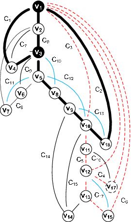
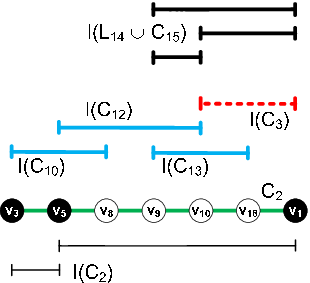
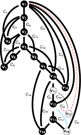
A running example of the algorithm.
A New Certifying 3-Connectivity Test.
It remains to deal with the case when the input graph is not -connected. For simplicity, we assume to be -connected, although the chain decomposition can check this fact. If is not -connected, the described algorithm fails to add a BG-path due to Theorem 2 when processing some chain, say . Therefore, after the processing phase for , must still contain a chain . Let be the segment containing and let be the set of segments that map to the connected component of the interval overlap graph containing . Then the union of dependent paths of the segments in is a path and the two extremal attachment points on of segments in build a separation pair. This pair certifies that is not -connected and can be computed in linear time.
Appendix A Omitted Proofs
We give the omitted proofs and the preparatory lemmas that lead to them.
Lemma 18 (aka Lemma 8).
Computing a chain decomposition of a -connected graph and classifying each chain with Algorithm 1 takes running time .
Proof.
The DFS tree can be obtained in time . The subdivision can be found in time linearly dependent on by taking two arbitrary backedges and with being the root of and finding the lowest common ancestor of and by traversing upwards. The computation of each remaining chain , , takes time linearly dependent on its length, too, which gives a running time of for the chain decomposition.
In order to obtain a fast classification in Algorithm 1, we store the following information on each chain : A pointer to its parent (for ), pointers to and and the information whether is a backedge. In addition, for each inner vertex of a pointer to is stored. That allows us to check vertices on being contained as inner vertices or end vertices in arbitrary chains in . If , we can check the condition on being of type in constant time by testing whether and are contained in . If , we check in constant time whether and are contained in . The condition for type needs constant time as well. Every chain is marked at most once, therefore unmarked as most once in line 15 of Algorithm 1, which gives a total running time of . ∎
Lemma 19.
Let be upwards-closed and modular. Then a BG-path for is a chain if and only if is upwards-closed and modular.
Proof.
If is a chain, is contained in and must be upwards-closed and modular due to the DFS structure. If is not a chain, we assume to the contrary that is upwards-closed and modular. Then must be the union of chains; let be the first chain in . Now cannot start with , since is in and property 1.1 contradicts . Thus, starts with , which contradicts as well, as is upwards-closed and a second chain in would include another backedge in at a vertex that is already incident to two DFS tree edges.∎
Lemma 19 shows that this restriction implies every BG-path to be a chain.
Lemma 20.
Proof.
For the first claim, assume to the contrary that violates property 1.3. Then must hold and follows. Let and be the parallel links of that contain the end vertices of as inner vertices, respectively. At least one of them, say , contains a backedge, since otherwise would contain a cycle. Let be the chain in that contains . Since contains exactly one backedge, is an end vertex of . If , must contain a backedge, as is an inner real vertex of . In that case, all inner vertices of lie in a subtree of that cannot be reached by due to property 1.1 and being upwards-closed. Thus, and with the same argument holds. With ( R 2 ), must be and , which contradicts our assumption.

We show that chains of type help to find BG-paths efficiently (Lemma 10) as part of the following Lemma.
Lemma 21 (aka Lemma 10).
Proof.
Assume to the contrary that is not of type and . Because is contained in , must be in as well. But then would be of type , since . Therefore, if is not of type , holds and must start with a backedge. Then the definition of the parent relation implies that is an inner vertex of .
For the second claim, let first be of type . Since is upwards-closed, modular and contains , satisfies the property 1.1 of BG-paths. In addition, holds by definition and with , must be an inner vertex of the path (see Figure 6). Therefore, the only chains that contain and are different from and fulfill . This implies having property 1.2. Using Lemma 20, is a BG-path for that preserves ( R 1 ) and ( R 2 ).
If is of type , property 1.1 follows from the same argument as before. Additionally, the inner real vertex in prevents any link containing and from having or as an inner vertex and therefore ensures property 1.2. Lemma 20 implies that is a BG-path for and must preserve ( R 1 ) and ( R 2 ), the latter due to the inner real vertex in . ∎
Proposition 22.
Every caterpillar consists of exactly one chain of type , namely the chain , and one or more chains of type .
Lemma 23.
is partitioned into single chains of types , , and the chains being contained in caterpillars. Moreover, no chain is contained in two caterpillars.
Proof.
With Proposition 22, it remains to show that every chain of type or is contained in exactly one caterpillar. If is of type , is part of the caterpillar (see Algorithm 1, line 13) and will not be assigned to a second caterpillar afterwards, as it is not marked. Otherwise, is of type and was therefore marked. We show that, after all chains in have been classified, is not marked anymore. This forces to be contained in exactly one caterpillar, as the only way to unmark chains is to assign them to a caterpillar (see Algorithm 1, line 15) and no chain is marked twice.
Let be the parent of . Because is of type , holds and is not a backedge, implying that the last edge of is in . Let be the end vertex of different from . Using Lemma 21, holds and is an inner vertex of . Then at least one backedge with must enter , since otherwise and would be a separation pair of . Let be the minimal chain with respect to that contains such a backedge.
As holds , the vertex is an inner vertex of , implying that is not of type . In addition, is not of type , since contains edges from and . At the time is found in the chain decomposition, every chain that already ends at a vertex in starts at and is therefore of type or . Since chains that are backedges cannot have children, the parent of is marked and is of type . Moreover, every chain corresponding to an inner vertex of the path is marked. This concludes to become unmarked due to line 15 of Algorithm 1. ∎
The following gives the detailed proof of Lemma 12.
Lemma 24 (aka Lemma 12).
Proof.
Let be good and let be the last vertex of the minimal chain in , thus . We assume at first that is a proper ancestor of (see Figure 3(b)). Then the path fulfills properties 1.1 and 1.2 and is a BG-path for with Lemma 20. Adding preserves to be upwards-closed but not modular. The restriction ( R 2 ) is also preserved, as is real and, for , must be either or , implying that becomes an inner real vertex of . Successively, for each chain of the chains in , we now add , which is a BG-path yielding an upwards-closed subdivision for analogue reasons.
Now assume that is a descendant of (see Figure 3(a)). Then and since is good, there is a real vertex strictly between and in . We first show that contains an inner real vertex as well. Assume the contrary. Then must be of type and has been added before, contradicting restriction ( R 2 ) unless . But must be different from , since exists, and it follows that contains an inner real vertex . Let be the parent of . Then is a BG-path due to the real vertices and and we add it, although it neither preserves to be upwards-closed nor modular. We next add , which restores upwards-closedness. The resulting subdivisions and both satisfy ( R 2 ), as is real in and and is real in . We proceed with adding successively paths, namely for each chain of the remaining chains in the path . With the same line of argument, these paths obtain upwards-closed subdivisions , each of which satisfies ( R 2 ).
In both cases, is modular, since is a list of chains. Moreover, the chosen BG-paths preserve ( R 1 ), as the chains in are of types and only, holds and is upwards-closed. All paths can be computed in time linearly dependent on the total number of edges in .
For the only if part, let and be the first two BG-paths in a decomposition of the chains in ; these exist, since holds in every caterpillar. Let be bad, as otherwise the claim follows. Then . We show that cannot be bad, as contains a real vertex in strictly between and . Because of properties 1.1 and 1.2, must hold and is a link of being parallel to . Since only the chain of type in starts at , both end vertices of must be different from . Then, due to properties 1.1 and 1.2, joins inner vertices of the parallel links and in , contradicting property 1.3, as . ∎
Lemma 25.
Let be a chain of type such that , and is minimal among the chains of type in its segment . Let be all ancestors of in with and being the minimal chain in . Then all chains can be successively added as BG-paths preserving ( R 1 ) and ( R 2 ) (possibly being part of caterpillars), unless one of the following exceptions holds:

Proof.
Let . Then is not of type by assumption and not of type , as chains of that type cannot have children. Assume that is of type and let be the caterpillar containing due to Lemma 23. If , holds, as otherwise would not be the chain of type in . But then contradicts the minimality of , since is not contained in and of type . We conclude that every chain in of type is contained in and forces to be of type . This is used in the following case distinction.
Let be of type . If , is a BG-path for with Lemma 21 and the claim follows. Otherwise, and all chains in are of type . Then is a proper ancestor of , since and is not of type . Moreover, is a proper ancestor of , because otherwise is a separation pair of due to the minimality of . It follows that is an inner vertex of . If , must contain , because is of type and a child of . Therefore, the edge joining with the parent of in is contained in . But since is upwards-closed, is also contained in , contradicting that . Thus, . If contains an inner real vertex, and can be subsequently added as BG-paths with Lemma 21, otherwise 25.1 is satisfied.
Let be of type . Then all chains in that are of type must be contained in . Since every caterpillar contains the parent of the chain and since contains no chain in due to ( R 1 ), holds and is of type with . Let with be the minimal chain in . If and is good, all chains in can be decomposed to BG-paths according to Lemma 12. If and is bad, 25.2 is satisfied. Only the case remains. Then is of type and, using the same arguments as in the case for type , is an inner vertex of and . If contains an inner real vertex, Lemmas 21 and 12 imply that and can be iteratively added as set of successive BG-paths, preserving ( R 1 ) and ( R 2 ). Otherwise, 25.3 is satisfied. ∎
We extend Lemma 25 to non-minimal chains of type .

Lemma 26.
Proof.
Using Lemma 25, we add the chains in as BG-paths. This partitions into new segments; let be such a new segment. If does not contain chains of type that start in , the claim follows for such chains in . Otherwise, let be the minimal chain of type in that starts in and let be its ancestors in . We show that is not contained in one of the exceptions 25.1-25.3 and can therefore be added as BG-path with Lemma 25, along with its proper ancestors in . First, assume to the contrary that is contained in exception 25.1 or 25.3 (see Figure 8(a)). Because is a proper descendant of and is of type , cannot be an inner vertex of , contradicting the assumption. Now assume to the contrary that is contained in exception 25.2 (see Figure 8(b)). Then is of type and part of a bad caterpillar , whose parent is not contained in . Because contains only chains in , must be a descendant of and is therefore contained in . Since is bad, is contained in and it follows with that must end in at the vertex . As is the only chain in that ends in , must hold. But this contradicts being bad, as contains the inner real vertex . Thus, and its ancestors in can be added, partitioning into smaller segments. Iterating the same argument for these segments establishes the claim for all chains of type in that start in . ∎
The next lemma shows that the only chains of type that cannot be added are either backedges or are contained as in exceptions 25.1-25.3.
Lemma 27.
Proof.
Let be the segment of and assume that is not a backedge. We first show that contains a chain of type that starts in . We can assume that is not contained in the exceptions 25.1 and 25.3, as then would contain such a chain by definition. Let be the last but one vertex in . Since is -connected, there is a minimal chain entering such that is an inner vertex of , as otherwise the inner vertices of would be separated by . By definition of the chain decomposition, must be of type or . Because is not contained in exceptions 25.1 and 25.3 and cannot contain exception 25.2, Lemma 25 can be applied on , obtaining the last claim. ∎
Here we give the proof of the key theorem (Theorem 15) of the paper.
Theorem 28 (aka Theorem 15).
For a subdivision , let be a chain such that holds for every proper ancestor of . Then all chains in and their proper ancestors that are not already contained in can be successively added as BG-paths (possibly being part of caterpillars) such that ( R 1 ) and ( R 2 ) is preserved. Moreover, the chains in that are contained in segments in which the minimal chain is not contained in can be added at any point in time in arbitrary order (together with their proper ancestors that are not contained in ).
Proof.
By assumption, is contained in . Let be a child of . If , must be of type . Let . Then cannot be of type , as otherwise it would be contained in due to ( R 1 ) and . It is neither of type , since in that case is contained in a proper ancestor of , implying by assumption. We conclude that is of type or and focus on the cases where can not be added. Let be the path on which depends on. If is of type , does not contain an inner real vertex, as otherwise can be added as BG-path due to Lemma 21. With Lemma 27, must be either a backedge or be contained as the minimal chain in exception 25.1 or 25.3. If is of type , is real and neither nor an inner vertex in can be real, since otherwise can be added as BG-path, preserving ( R 1 ) and ( R 2 ). If is of type , is the minimal chain of a caterpillar with parent . According to Lemma 12, is bad and, thus, corresponds to exception 25.2. The following is a list of the possible cases for which a child of is not added.
- 1.
- 2.
and is of type without a real vertex in
- 3.
We iteratively add all chains in that do not satisfy one of the above three cases 15.1-15.3 for and whose segments do not contain one of the exceptions 25.1-25.3 for (the latter followed by adding the proper ancestors in the segment of according to Lemma 26). Let be the set of remaining chains in and let be the set of remaining chains in . If , holds as well, as otherwise the minimal chain in the segment containing one of the exceptions 25.1-25.3 is a child of , contradicting . This implies the claim for .
We prove the theorem by showing that must hold. Assume to the contrary that and let be the current subdivision (all segments will be dependent on ). Then must contain a link of length at least two, because the dependent path in each of the cases 15.1-15.3 is in and contains a non-real vertex due to the -connectivity and simpleness of . According to Lemma 4, contains an inner vertex on which a BG-path starts (not necessarily being a chain and not necessarily preserving ( R 1 ) or ( R 2 )). Let be the first edge of . Then is not contained in the segment of any , as otherwise would not have property 1.2, because is non-real and all start vertices of the chains in the segment of that are in are contained in . Thus, cannot be a child of and it follows that . In particular, is not of type .
The segment of cannot contain a chain of type that starts in , as it otherwise contains a chain of type or due to exceptions 25.1-25.3, contradicting the previous argument. In particular, is not of type and the only remaining case is that is of type .
Let be the maximal ancestor of that is not of type . Then holds by construction of the chain decomposition and must be contained in the segment of due to ( R 1 ), ( R 2 ) and being non-real. Since the segment of cannot contain a chain of type that starts in , must be of type . But then, as is an inner vertex of , must be a child of , contradicting that is not contained in the segment of any . This is a contradiction to the existence of and it follows that , which implies the claim. ∎
References
- [1] S. Albroscheit. Ein Algorithmus zur Konstruktion gegebener 3-zusammenhängender Graphen (in German). Diploma thesis, Freie Universität Berlin, 2006.
- [2] D. W. Barnette and B. Grünbaum. On Steinitz’s theorem concerning convex 3-polytopes and on some properties of 3-connected graphs. Many Facets of Graph Theory, Lecture Notes in Mathematics, 110:27–40, 1969.
- [3] V. Batagelj. Inductive classes of graphs. In Proceedings of the 6th Yugoslav Seminar on Graph Theory, pages 43–56, Dubrovnik, 1986.
- [4] V. Batagelj. An improved inductive definition of two restricted classes of triangulations of the plane. In Combinatorics and Graph Theory, Banach Center Publications, volume 25, pages 11–18. PWN Warsaw, 1989.
- [5] G. D. Battista and R. Tamassia. On-line graph algorithms with SPQR-trees. In Proceedings of the 17th International Colloquium on Automata, Languages and Programming (ICALP’90), pages 598–611, 1990.
- [6] P. Bertolazzi, G. D. Battista, C. Mannino, and R. Tamassia. Optimal upward planarity testing of single-source digraphs. SIAM J. Comput., 27(1):132–169, 1998.
- [7] M. Blum and S. Kannan. Designing programs that check their work. In Proceedings of the 21st Annual ACM Symposium on Theory of Computing (STOC’89), pages 86–97, New York, 1989.
- [8] N. Chiba and T. Nishizeki. The Hamiltonian cycle problem is linear-time solvable for 4-connected planar graphs. J. Algorithms, 10(2):187–211, 1989.
- [9] A. Elmasry, K. Mehlhorn, and J. M. Schmidt. A linear-time certifying triconnnectivity algorithm for Hamiltonian graphs, preprint available at http://www.mpi-inf.mpg.de/~mehlhorn/ftp/Hamilton.pdf.
- [10] Z. Galil and G. F. Italiano. Reducing edge connectivity to vertex connectivity. SIGACT News, 22(1):57–61, 1991.
- [11] M. R. Garey, D. S. Johnson, and R. E. Tarjan. The planar Hamiltonian circuit problem is NP-complete. SIAM J. Comput., 5(4):704–714, 1976.
- [12] C. Gutwenger, P. Mutzel, and R. Weiskircher. Inserting an edge into a planar graph. In Proceedings of the 12th Annual ACM-SIAM Symposium on Discrete Algorithms (SODA’01), pages 246–255, 2001.
- [13] J. E. Hopcroft and R. E. Tarjan. Dividing a graph into triconnected components. SIAM J. Comput., 2(3):135–158, 1973.
- [14] E. L. Johnson. A proof of the four-coloring of the edges of a regular three-degree graph. Technical report, O. R. C. 63-28 (R. R.) Min. Report, Univ. of California, Operations Research Center, 1963.
- [15] D. Kratsch, R. M. McConnell, K. Mehlhorn, and J. P. Spinrad. Certifying algorithms for recognizing interval graphs and permutation graphs. SIAM J. Comput., 36(2):326–353, 2006. Preliminary version in SODA 2003, pp. 158–167.
- [16] K. Mehlhorn and S. Näher. From algorithms to working programs: On the use of program checking in LEDA. In Proceedings of the 23rd International Symposium on Mathematical Foundations of Computer Science (MFCS’98), pages 84–93, 1998.
- [17] K. Mehlhorn, S. Näher, M. Seel, R. Seidel, T. Schilz, S. Schirra, and C. Uhrig. Checking geometric programs or verification of geometric structures. Comput. Geom. Theory Appl., 12(1-2):85–103, 1999.
- [18] P. Mutzel. The SPQR-tree data structure in graph drawing. In Proceedings of the 30th International Colloquium on Automata, Languages and Programming (ICALP’03), pages 34–46, 2003.
- [19] S. Olariu and A. Y. Zomaya. A time- and cost-optimal algorithm for interlocking sets – With applications. IEEE Trans. Parallel Distrib. Syst., 7(10):1009–1025, 1996.
- [20] J. M. Schmidt. Construction sequences and certifying 3-connectedness. In Proceedings of the 27th International Symposium on Theoretical Aspects of Computer Science (STACS’10), Nancy, France, pages 633–644, 2010.
- [21] C. Thomassen. Kuratowski’s theorem. Journal of Graph Theory, 5(3):225–241, 1981.
- [22] C. Thomassen. Reflections on graph theory. Journal of Graph Theory, 10(3):309–324, 2006.
- [23] W. T. Tutte. A theorem on planar graphs. Trans. Amer. Math. Soc., 82:99–116, 1956.
- [24] W. T. Tutte. A theory of 3-connected graphs. Indag. Math., 23:441–455, 1961.
- [25] W. T. Tutte. Connectivity in graphs. In Mathematical Expositions, volume 15. University of Toronto Press, 1966.
- [26] K.-P. Vo. Finding triconnected components of graphs. Linear and Multilinear Algebra, 13:143–165, 1983.
- [27] K.-P. Vo. Segment graphs, depth-first cycle bases, 3-connectivity, and planarity of graphs. Linear and Multilinear Algebra, 13:119–141, 1983.