On Beamformer Design for Multiuser MIMO Interference ChannelsThanks: Juho Park and Youngchul Sung are with the Dept. of Electrical Engineering, KAIST, Daejeon 305-701, South Korea. E-mail:{jhp@ and ysung@ee.}kaist.ac.kr and H. Vincent Poor is with Dept. of Electrical Engineering, Princeton University, Princeton, NJ 08544, E-mail:poor@princeton.edu. This work was supported by the Korea Research Foundation Grant funded by the Korean Government (KRF-2008-220-D00079).

Juho Park Student Member, IEEE Youngchul Sung^† ^†^†thanks: ^†Corresponding author Senior Member, IEEE and Affiliation: H. Vincent Poor, Fellow, IEEE

Abstract

This paper considers several linear beamformer design paradigms for multiuser time-invariant multiple-input multiple-output interference channels. Notably, interference alignment and sum-rate based algorithms such as the maximum signal-to-interference-plus noise (max-SINR) algorithm are considered. Optimal linear beamforming under interference alignment consists of two layers; an inner precoder and decoder (or receive filter) accomplish interference alignment to eliminate inter-user interference, and an outer precoder and decoder diagonalize the effective single-user channel resulting from the interference alignment by the inner precoder and decoder. The relationship between this two-layer beamforming and the max-SINR algorithm is established at high signal-to-noise ratio. Also, the optimality of the max-SINR algorithm within the class of linear beamforming algorithms, and its local convergence with exponential rate, are established at high signal-to-noise ratio.

Index Terms:

Multiuser MIMO, interference channels, interference alignment, two-layer linear beamforming, max-SINR algorithm, sum rate, fixed point, convergence.

I Introduction

Since interference alignment was shown in [1] to achieve the maximum number of degrees of freedom (DoF) in $K$ -user (possibly time-varying) interference channels, this technique has attracted considerable attention as a candidate for handling interference in multiuser wireless environments. With interference alignment, each user achieves almost half of the capacity achievable without interference and the total sum rate of the system is given by

C=\frac{K}{2}\log(\mbox{SNR})+o(\log(\mbox{SNR})),

(1)

where the $o(\log(\mbox{SNR}))$ term decays faster than $\log(\mbox{SNR})$ as the signal-to-noise ratio (SNR) increases. Interference alignment can be classified into two categories: signal level (or scale) alignment [2, 3, 4, 5, 6, 7, 8] and signal space alignment [1, 9, 10, 11, 12]. (For a nice survey of the literature in this area, see [13].) While the alignment in signal scale lends tractability to DoF characterization, interference alignment in signal space provides an attractive way to realize interference alignment in practice. The signal space can be generated in several ways, such as by concatenating time symbols or frequency bins as in [1] when the channel is varying over time or frequency, or by using multiple-input multiple-output (MIMO) antenna techniques. Of these two approaches, MIMO techniques seem to be more robust and attractive for realistic slowly-fading wireless channels [13]. While much work has been done on the feasibility analysis and DoF characterization of interference alignment, in this paper we focus on the algorithmic aspect of interference alignment in signal space based on MIMO antennas in time-invariant channels. Up to now, several algorithms have been proposed to design interference-aligning beamforming matrices at transmitters and receivers for the practical setting of time-invariant MIMO interference channels [14, 15, 16, 17, 18]. While these approaches design interference-aligning beamforming matrices, others have proposed algorithms to maximize the sum rate directly since interference alignment is optimal at high SNR and optimal only in terms of DoF even then, i.e., the $o(\log(\mbox{SNR}))$ term still exists in the sum rate achieved by interference alignment. Among these latter types of algorithms, the max-SINR algorithm of Gomadam et al. [14] and the sum-rate gradient algorithm of Sung et al. [18] are noticeable and promising. Whereas the latter is based on the gradient descent of the sum rate as a cost function, the former is based on the idea of channel reciprocity and also on the individual stream approach rather than on the individual user approach aggregating multiple streams of a single user. Although Gomadam et al. proposed the max-SINR algorithm, its overall optimality and behavior were not explored fully in [14]. In this paper, we investigate the relationship among three beamformer design algorithms: interference alignment, max-SINR and sum-rate gradient algorithms, and show the optimality of the max-SINR algorithm within the class of linear beamforming algorithms at high SNR. Optimizing the beamforming filters for multiuser time-invariant MIMO interference channels is not a simple problem as noted in [14], and the analysis of such algorithms as the max-SINR algorithm is not a trivial task either due to the nonconvex nature of the problem. Our approach to this analytical task is based on fixed point analysis [19]. It is not difficult to show that optimal linear beamforming under interference alignment consists of two layers composed of inner and outer layers, which was independently derived in [18]. An inner precoder and decoder^†^† † We will use the term ’linear decoder’ or simply ’decoder’ for the receive filter in this paper. accomplish interference alignment to eliminate inter-user interference, and an outer precoder and decoder diagonalize the effective single-user channel resulting from the interference alignment by the inner precoder and decoder. Based on fixed point analysis, we have shown the following properties of the considered algorithms and the relationship among them.

(i)

At high SNR, all fixed points of the max-SINR algorithm with a DoF guarantee are optimal two-layer beamformers as noted above.
(ii)

The set of fixed points of the max-SINR algorithm includes the globally optimal linear beamformer at high SNR.
(iii)

Any interference-aligning precoder is a fixed point of the sum-rate gradient algorithm regardless of the optimality of the outer precoder and decoder.
(iv)

Finally, at high SNR, the max-SINR algorithm converges exponentially to a fixed point when it is initialized within a neighborhood of the fixed point.

Thus, the max-SINR algorithm is optimal within the class of linear beamforming algorithms at high SNR in the sense of (ii). Comparing (i) and (iii), the max-SINR algorithm has advantage over the sum-rate gradient algorithm in that it yields not only interference alignment but also optimal outer coders at high SNR. This is because the max-SINR algorithm is based on a stream-by-stream approach and this individual stream approach adds resolving power to the max-SINR algorithm compared with the user-by-user algorithms.

This paper is organized as follows. The data model and background are described in Section II. In Section III, we explain the two-layer linear precoder and decoder structure for MIMO interference channels. In Section IV, we investigate the properties of the sum-rate based beamformer design algorithms and the relationship with the two-layer linear beamforming structure of Section III. In Section V we provide some numerical results, followed by conclusions in Section VI.

Notation

We will make use of standard notational conventions. Vectors and matrices are written in boldface with matrices in capitals. All vectors are column vectors. For a matrix ${\bf A}$ , ${\bf A}^{T}$ and ${\bf A}^{H}$ indicate the transpose and Hermitian transpose of ${\bf A}$ , respectively, and $\mbox{rank}({\bf A})$ represents the rank of ${\bf A}$ . ${\cal C}({\bf A})$ represents the column space of ${\bf A}$ , i.e., the linear subspace spanned by the columns of ${\bf A}$ . $|{\bf A}|$ and ${\bf A}^{\dagger}$ denote the determinant and Moore-Penrose pseudo-inverse of ${\bf A}$ , respectively. For a linear subspace ${\cal S}$ , $\mbox{dim}({\cal S})$ denotes the dimension of ${\cal S}$ , and ${\cal S}^{\perp}$ represents the orthogonal complement of ${\cal S}$ . ${\bf I}_{n}$ stands for the identity matrix of size $n$ (the subscript is included only when necessary). For a vector ${\bf a}$ , $\|{\bf a}\|$ represents the 2-norm of ${\bf a}$ . The notation ${\bf x}\sim{\cal N}(\hbox{\boldmath$\mu$\unboldmath},\hbox{$\bf\Sigma$})$ means that the random vector ${\bf x}$ is complex Gaussian with mean vector $\mu$ and covariance matrix $\bf\Sigma$ . ${\mathbb{E}}\{{\bf x}\}$ denotes the expectation of ${\bf x}$ . ${{\mathscr{A}}}\setminus{{\mathscr{B}}}$ denotes the relative complement of a set ${{\mathscr{A}}}$ in another set ${{\mathscr{B}}}$ .

II Data Model and Background

We consider a $K$ -user $M\times M$ MIMO interference channel in which $K$ transmitters each having $M$ antennas simultaneously transmit to $K$ receivers each also having $M$ antennas, as shown in Figure 1. Due to interference each receiver receives the desired signal from its corresponding transmitter and also interference from other undesired transmitters. Thus, the received signal vector at receiver $k$ at symbol time $t$ is given by

	$\displaystyle{\bf y}_{k}(t)$	$\displaystyle=$	$\displaystyle{\bf H}_{kk}(t){\bf V}_{k}(t){\bf s}_{k}(t)+\sum_{l\neq k}{\bf H}_{kl}(t){\bf V}_{l}(t){\bf s}_{l}(t)+{\bf n}_{k}(t),$		(2)
		$\displaystyle=$	$\displaystyle{\bf H}_{kk}(t)({\bf v}_{k}^{(1)}(t)s_{k}^{(1)}(t)+\cdots+{\bf v}_{k}^{(d_{k})}(t)s_{k}^{(d_{k})}(t))+\sum_{l\neq k}{\bf H}_{kl}(t){\bf V}_{l}(t){\bf s}_{l}(t)+{\bf n}_{k}(t),$		(2)

where ${\bf{H}}_{kl}(t)$ is an $M\times M$ channel matrix from transmitter $l$ to receiver $k$ at symbol time $t$ , ${{\bf V}}_{k}(t)=[{\bf v}_{k}^{(1)}(t),{\bf v}_{k}^{(2)}(t),\cdots,{\bf v}_{k}^{(d_{k})}(t)]$ is an $M\times d_{k}$ transmit beamforming matrix, ${{\bf s}}_{k}(t)$ $=[s_{k}^{(1)}(t),$ $\cdots,$ $s_{k}^{(d_{k})}(t)]^{T}$ is a $d_{k}$ -dimensional transmit signal vector, $d_{k}$ is the number of data streams for user $k$ , and ${\bf{n}}_{k}(t)$ is an $M\times 1$ circularly symmetric complex Gaussian noise vector with distribution ${\cal N}({\mathbf{0}},{\bf I}_{M})$ . The spatial signature ${\bf v}_{k}^{(m)}(t)$ of the $m$ -th stream of user $k$ has unit norm. We assume that $s_{k}^{(m)}(t)$ , $m=1,2,\cdots,d_{k}$ , are independent and ${\mathbb{E}}\{|s_{k}^{(m)}(t)|^{2}\}=P_{k}^{(m)}$ for all $t=1,2,\cdots$ , and the total transmit power of the overall system is given by

P_{t}=\sum_{k=1}^{K}\sum_{m=1}^{d_{k}}P_{k}^{(m)}.

(3)

We assume that the channels are time-invariant, i.e., the channel matrices $\{{\bf H}_{kl}(t)\}$ do not change over time. Thus, we omit the time index $t$ from here on. We also assume that channel information is known to all of the transmitters and the receivers. Further, in this paper we consider the case of $d=d_{1}=d_{2}=\cdots=d_{K}=M/2$ to allow for a maximum number of degrees.

Refer to caption — Fig. 1: $K$ -user MIMO interference channel model.

II-A Background

In this subsection, we briefly recapitulate those results of the previous works [14] and [18] that are relevant to the analysis in the sequel.

II-A1 Interference alignment in signal space

The basic idea of interference alignment via the signal space approach [1] is to confine the interference from the undesired transmitters within a linear subspace at the receiver of dimension less than that of the received signal space so that the remaining subspace can be used for interference-free communication. Thus, the interference alignment condition is given as follows [14, 13].

Condition 1

There exist non-zero matrices $\{{\bf U}_{k}:\mbox{size}({\bf U}_{k})=M\times d,~\mbox{rank}({\bf U}_{k})=d,~~k=1,2,\cdots,K\}$ and $\{{\bf V}_{l}:\mbox{size}({\bf V}_{l})=M\times d,~\mbox{rank}({\bf V}_{l})=d,~~l=1,2,\cdots,K\}$ such that

	$\displaystyle{\bf U}_{k}^{H}{\bf{H}}_{kl}{\bf{V}}_{l}$	$\displaystyle=$	$\displaystyle{\mathbf{0}},~~k\in{\mathscr{K}}\stackrel{{\scriptstyle\Delta}}{{=}}\{1,2,\cdots,K\},~l\in{\mathscr{K}}\setminus\{k\},$		(4)
	$\displaystyle\mbox{and ~rank}({\bf U}_{k}^{H}{\bf H}_{kk}{\bf V}_{k})$	$\displaystyle=$	$\displaystyle d,~~k\in{\mathscr{K}}.$		(5)

Here, ${\bf V}_{k}$ and ${\bf U}_{k}=[{\bf u}_{k}^{(1)},\cdots,{\bf u}_{k}^{(d)}]$ are the transmit beamforming matrix (or linear precoder) and receive beamforming matrix (or linear decoder), respectively, of user $k$ . Thus, when interference alignment is achieved by the transmit and receive beamforming matrices $\{{\bf V}_{k}\}$ and $\{{\bf U}_{k}\}$ , ${\cal C}({\bf U}_{k})$ is the orthogonal complement of the aligned interference subspace generated by $\sum_{l\neq k}{\bf H}_{kl}{\bf V}_{l}{\bf s}_{l}$ at user $k$ , and we have the following interference covariance matrix and its singular value decomposition (SVD):

	$\displaystyle{\bf Z}_{k}$	$\displaystyle\stackrel{{\scriptstyle\Delta}}{{=}}$	$\displaystyle\sum_{l\neq k}{\bf H}_{kl}{\bf V}_{l}\mbox{diag}(P_{l}^{(1)},\cdots,P_{l}^{(d)}){\bf V}_{l}^{H}{\bf H}_{kl}^{H},$		(6)
		$\displaystyle=$	$\displaystyle\hbox{$\bf\Gamma$}_{k}\mbox{diag}(\sigma_{k1},\cdots,\sigma_{kd},0,\cdots,0)\hbox{$\bf\Gamma$}_{k}^{H}.$		(6)

Also, by Hermitian transposing (4) and summing the terms over $k$ , we have $\sum_{k\neq l}{\bf V}_{l}^{H}{\bf H}_{kl}^{H}{\bf U}_{k}$ $=$ ${\bf V}_{l}^{H}\sum_{k\neq l}$ $({\bf H}_{kl}^{H}{\bf U}_{k})=0$ and

	$\displaystyle\overleftarrow{{\bf Z}}_{l}$	$\displaystyle\stackrel{{\scriptstyle\Delta}}{{=}}$	$\displaystyle\sum_{k\neq l}\overleftarrow{{\bf H}}_{lk}{\bf U}_{k}\mbox{diag}(\overleftarrow{P}_{k}^{(1)},\cdots,\overleftarrow{P}_{k}^{(d)}){\bf U}_{k}^{H}\overleftarrow{{\bf H}}_{lk},$		(7)
		$\displaystyle=$	$\displaystyle\overleftarrow{\hbox{$\bf\Gamma$}}_{k}\mbox{diag}(\overleftarrow{\sigma}_{k1},\cdots,\overleftarrow{\sigma}_{kd},0,\cdots,0)\overleftarrow{\hbox{$\bf\Gamma$}}_{k}^{H},$		(7)

where $\overleftarrow{{\bf H}}_{lk}={\bf H}_{kl}^{H}$ and $\overleftarrow{P}_{k}^{(m)}$ is the power associated with ${\bf u}_{k}^{(m)}$ . There exist efficient algorithms to obtain interference aligning beamforming matrices, e.g., [14, 15, 16], and thus interference-aligning beamforming matrices $\{{\bf U}_{k},{\bf V}_{k}\}$ can be acquired easily using such algorithms.

II-A2 Sum rate and the related algorithms

Although interference alignment achieves the maximum number of degrees of freedom in multiuser MIMO interference channels, i.e., the rate achieved by interference alignment is within a constant gap from the capacity regardless of the value of SNR at high SNR, larger sum rate can be achieved by linear sum-rate maximizing beamforming at low and intermediate SNR and even at high SNR. Consider the $m$ -th stream of user $k$ and the corresponding received signal at receiver $k$ given by

{\bf y}_{k}={\bf H}_{kk}{\bf v}_{k}^{(m)}s_{k}^{(m)}+\sum_{j\neq m}{\bf H}_{kk}{\bf v}_{k}^{(j)}s_{k}^{(j)}+\sum_{l\neq k}{\bf H}_{kl}{\bf V}_{l}{\bf s}_{l}+{\bf n}_{k},

(8)

where the covariance matrix of the overall interference and noise for this stream is given by

{\bf R}_{k}^{(m)}\stackrel{{\scriptstyle\Delta}}{{=}}\sum_{l=1}^{K}\sum_{j=1}^{d}P_{l}^{(j)}{\bf H}_{kl}{\bf v}_{l}^{(j)}{\bf v}_{l}^{(j)H}{\bf H}_{kl}^{H}-P_{k}^{(m)}{\bf H}_{kk}{\bf v}_{k}^{(m)}{\bf v}_{k}^{(m)H}{\bf H}_{kk}^{H}+{\bf I}.

(9)

Thus, the signal-to-interference-plus-noise ratio (SINR) maximizing receiver filter ${\bf u}_{k}^{(m)}$ for this stream is given by the whitened matched filter [20]:

{{\bf u}}_{k}^{(m)}=\frac{({\bf R}_{k}^{(m)})^{-1}{\bf H}_{kk}{\bf v}_{k}^{(m)}}{\|({\bf R}_{k}^{(m)})^{-1}{\bf H}_{kk}{\bf v}_{k}^{(m)}\|}

(10)

(the normalization for unit norm does not affect the SINR) and the corresponding rate for the stream is given by

C_{k}^{(m)}=\log\left(1+P_{k}^{(m)}{\bf v}_{k}^{(m)H}{\bf H}_{kk}^{H}({\bf R}_{k}^{(m)})^{-1}{\bf H}_{kk}{\bf v}_{k}^{(m)}\right).

(11)

The overall sum rate of the system is given by

C=\sum_{k=1}^{K}\sum_{m=1}^{d}C_{k}^{(m)}.

(12)

Obtaining sum-rate maximizing transmit beam vectors $\{{\bf v}_{k}^{m},k=1,\cdots,K,m=1,\cdots,d\}$ is not a simple problem due to the nonconvex dependence structure of $C$ on ${\bf v}_{k}^{(m)}$ via $({\bf R}_{k}^{(m)})^{-1}$ in (11). Thus, several researchers have proposed iterative algorithms to design beamforming matrices for maximizing the sum rate of the system directly, e.g., [14, 18]. In [14], Gomadam et al. proposed the max-SINR algorithm to design sum-rate maximizing linear precoders and decoders based on the individual stream approach and on channel reciprocity suggested from the duality between the Gaussian multiple access channel (MAC) and the Gaussian broadcast channel (BC) [21, 22, 23]. The max-SINR algorithm based on the idea of reciprocity provides an effective method to design sum-rate maximizing linear precoders and decoders. The optimality and solution structure of this algorithm will be discussed in later sections.

The max-SINR algorithm (Gomadam et al. [14])

Step 1.

Fix $\{P_{k}^{(m)},k=1,\cdots,K,~m=1,\cdots,d\}$ such that $P_{t}=\sum_{k=1}^{K}\sum_{m=1}^{d_{k}}P_{k}^{(m)}$ , and initialize $n=0$ and $\{{\bf v}_{k}^{(m)}[n]\}$ . (Equal power allocation was used in [14].)
Step 2.

(VU-step) Compute the receiver filters $\{{\bf u}_{k}^{(m)}[n]\}$ for all streams of all users from (9) and (10).

Step 3.

(UV-step) Exploiting channel reciprocity, compute $\{{\bf v}_{k}^{(m)}[n+1]\}$ by treating $\{{\bf u}_{k}^{(m)}[n]\}$ from Step 1 as the transmit vector and changing the role of transmitter and receiver. That is, obtain the interference-plus-noise covariance matrix in the reciprocal channel:

\overleftarrow{{\bf R}}_{k}^{(m)}[n]=\sum_{l=1}^{K}\sum_{j=1}^{d}\overleftarrow{P}_{l}^{(j)}\overleftarrow{{\bf H}}_{kl}{\bf u}_{l}^{(j)}[n]{\bf u}_{l}^{(j)}[n]^{H}\overleftarrow{{\bf H}}_{kl}^{H}-\overleftarrow{P}_{k}^{(m)}\overleftarrow{{\bf H}}_{kk}{\bf u}_{k}^{(m)}[n]{\bf u}_{k}^{(m)}[n]^{H}\overleftarrow{{\bf H}}_{kk}^{H}+{\bf I},

and

{{\bf v}}_{k}^{(m)}[n+1]=\frac{(\overleftarrow{{\bf R}}_{k}^{(m)}[n])^{-1}\overleftarrow{{\bf H}}_{kk}{\bf u}_{k}^{(m)}[n]}{\|(\overleftarrow{{\bf R}}_{k}^{(m)}[n])^{-1}\overleftarrow{{\bf H}}_{kk}{\bf u}_{k}^{(m)}[n]\|}.

(13)

Step 4.

Increase $n$ and iterate Steps 2 and 3.

Note that the max-SINR algorithm itself does not consider interference alignment but tries to increase the sum rate through designing better beamforming matrices to increase the stream SINR.

On the other hand, Sung et al. proposed a different iterative method to design sum-rate maximizing beamforming matrices based on the gradient descent method and user-by-user approach in [18], which we call the sum-rate gradient algorithm in this paper. Under the assumption of equal power allocation, the rate for user $k$ based on linear beamforming matrices $\{{\bf V}_{k}\}$ for the model (2) is given by

$\displaystyle C_{k}$	$\displaystyle=$	$\displaystyle\log\left\|{\bf I}+\frac{P_{t}}{Kd}({\bf I}+{\bf Z}_{k})^{-1}{\bf H}_{kk}{\bf V}_{k}{\bf V}_{k}^{H}{\bf H}_{kk}^{H}\right\|,$	(14)
	$\displaystyle=$	$\displaystyle\log\left\|({\bf I}+{\bf Z}_{k})^{-1}\left({\bf I}+{\bf Z}_{k}+\frac{P_{t}}{Kd}{\bf H}_{kk}{\bf V}_{k}{\bf V}_{k}^{H}{\bf H}_{kk}^{H}\right)\right\|,$	(15)
	$\displaystyle=$	$\displaystyle\log\left\|({\bf I}+{\bf Z}_{k})^{-1}\left({\bf I}+\frac{P_{t}}{Kd}\sum_{l=1}^{K}{\bf H}_{kl}{\bf V}_{l}{\bf V}_{l}^{H}{\bf H}_{kl}^{H}\right)\right\|,$	(16)
	$\displaystyle=$	$\displaystyle\log\left\|{\bf R}_{k}\right\|-\log\left\|{\bf I}+{\bf Z}_{k}\right\|,$	(17)

where the overall signal covariance matrix ${\bf R}_{k}$ for user $k$ is given by

{\bf R}_{k}\stackrel{{\scriptstyle\Delta}}{{=}}\sum_{l=1}^{K}\frac{P_{t}}{Kd}{\bf H}_{kl}{\bf V}_{l}{\bf V}_{l}^{H}{\bf H}_{kl}^{H}+{\bf I},

(18)

and the overall sum rate is given by

C=\sum_{k=1}^{K}C_{k}.

(19)

The direction of maximum increase of the functional $C({\bf V}_{1},\cdots,{\bf V}_{K})$ is given by the gradient of the functional $C({\bf V}_{1},\cdots,{\bf V}_{K})$ with respect to ${\bf V}_{k}^{o}$ , where ${\bf V}_{k}^{o}=({\bf V}_{k}^{H})^{T}$ , and it is obtained by the complex gradient operator [24, 25]:

\nabla_{{\bf V}_{k}^{o}}C({\bf V}_{1},\cdots,{\bf V}_{K})=\sum_{l=1}^{K}\left(\frac{\partial\log|{\bf R}_{l}|}{\partial{\bf V}_{k}^{o}}-\frac{\partial\log|{\bf I}+{\bf Z}_{l}|}{\partial{\bf V}_{k}^{o}}\right).

(20)

From the fact that for a matrix ${\bf C}$

\frac{\partial\log|{\bf C}(\{{\bf V}_{l}\})|}{\partial{\bf V}_{k}^{o}}=\mathrm{tr}\left\{{\bf C}(\{{\bf V}_{l}\})^{-1}\frac{\partial{\bf C}(\{{\bf V}_{l}\})}{\partial{\bf V}_{k}^{o}}\right\},

(21)

the gradient of the sum rate (19) with respect to ${\bf V}_{k}^{o}$ is given by

\nabla_{{\bf V}_{k}^{o}}C({\bf V}_{1},\cdots,{\bf V}_{K})=\sum_{l=1}^{K}\frac{P_{t}}{Kd}{\bf H}_{lk}^{H}{\bf R}_{l}^{-1}{\bf H}_{lk}{\bf V}_{k}-\sum_{l\neq k}\frac{P_{t}}{Kd}{\bf H}_{lk}^{H}({\bf I}+{\bf Z}_{l})^{-1}{\bf H}_{lk}{\bf V}_{k}.

(22)

An algorithm was constructed in [18] to update the beam based on the gradient and to converge at least to a local maximum. Note that the max-SINR algorithm is based on the stream-by-stream approach (8, 11, 12) whereas the sum rate gradient algorithm relies on the user-by-user approach (2, 14, 19). The resulting difference between the stream-by-stream and user-by-user approaches will be discussed in later sections.

III Two-Layer Linear Precoder and Decoder Structure
under Interference Alignment

In this section, we consider optimal beamforming matrix design under the interference alignment constraint, i.e., (4). As already noted in [14], [13] and [18], once interference-aligning beamforming matrices $\{\underline{{\bf U}}_{k}\}$ and $\{\underline{{\bf V}}_{k}\}$ are given, any other matrices that generate the same subspaces as $\{\underline{{\bf U}}_{k}\}$ and $\{\underline{{\bf V}}_{k}\}$ are also interference-aligning. That is, $\{{\bf V}_{k}:{\bf V}_{k}=\underline{{\bf V}}_{k}\mbox{${\bf\Phi}$}_{k},~\mbox{${\bf\Phi}$}_{k}\in{\mathbb{C}}^{d\times d},k\in{\mathscr{K}}\}$ and $\{{\bf U}_{k}:{\bf U}_{k}=\underline{{\bf U}}_{k}\hbox{$\bf\Theta$}_{k},~{\mathbf{\Theta}}_{k}\in{\mathbb{C}}^{d\times d},k\in{\mathscr{K}}\}$ are also interference aligning beamforming matrices for the given channel for any $\{\mbox{${\bf\Phi}$}_{k}\}$ and $\{\hbox{$\bf\Theta$}_{k}\}$ when $\{\underline{{\bf U}}_{k}\}$ and $\{\underline{{\bf V}}_{k}\}$ are interference-aligning. Thus, for a given interference-aligning subspaces or matrices $\{\underline{{\bf U}}_{k}\}$ and $\{\underline{{\bf V}}_{k}\}$ , the matrices $\{\mbox{${\bf\Phi}$}_{k}\}$ and $\{\hbox{$\bf\Theta$}_{k}\}$ can be optimized further to increase the overall sum rate.

Problem 1 (Optimization of linear precoder and decoder under interference alignment)

For given interference aligning subspaces given by the column spaces of $\{\underline{{\bf V}}_{k}\}$ and $\{\underline{{\bf U}}_{k}\}$ composed of orthonormal columns^‡^‡ ‡ The assumption of orthonormal columns does not result in any loss., design optimal $\{\mbox{${\bf\Phi}$}_{k}^{*}\in\mathbb{C}^{d\times d}\}$ and $\{\hbox{$\bf\Theta$}_{k}^{*}\in\mathbb{C}^{d\times d}\}$ to maximize the sum rate. Thus, optimal interference-aligning linear precoder and decoder are given by

{\bf V}_{k}^{*}=\underline{{\bf V}}_{k}\mbox{${\bf\Phi}$}_{k}^{*}\quad\mbox{and}\quad{\bf U}_{k}^{*}=\underline{{\bf U}}_{k}\hbox{$\bf\Theta$}_{k}^{*}.

(23)

The difference between Problem 1 and the classical MIMO beamforming problem is that in Problem 1 we have a restriction on the choice of beamforming matrices within the class of interference-aligning matrices, whereas the MIMO beamforming problem has no such constraint. However, the solution to Problem 1 is simple and here we present its solution for the purpose of later discussion. (It was also derived in [18].) Let ${\bf\Pi}_{k}=\underline{{\bf U}}_{k}$ be the first projection at receiver $k$ . Then, the projected signal at receiver $k$ is given by

$\displaystyle{\bf r}_{k}$	$\displaystyle=$	$\displaystyle{\bf\Pi}_{k}^{H}{\bf y}_{k},$	(24)
	$\displaystyle=$	$\displaystyle{\bf\Pi}_{k}^{H}{\bf H}_{kk}{\bf V}_{k}{\bf s}_{k}+{\bf\Pi}_{k}^{H}\sum_{l\neq k}{\bf H}_{kl}{\bf V}_{l}{\bf s}_{l}+{\bf\Pi}_{k}{\bf n}_{k},$	(25)
	$\displaystyle=$	$\displaystyle\underline{{\bf U}}_{k}^{H}{\bf H}_{kk}{\bf V}_{k}{\bf s}_{k}+\tilde{{\bf n}}_{k}.$	(26)

The second term on the right-handed side (RHS) of (25) disappears due to interference alignment. Substituting ${\bf V}_{k}=\underline{{\bf V}}_{k}\mbox{${\bf\Phi}$}_{k}$ into (26), we have

{\bf r}_{k}=\underline{{\bf U}}_{k}^{H}{\bf H}_{kk}\underline{{\bf V}}_{k}\mbox{${\bf\Phi}$}_{k}{\bf s}_{k}+\tilde{{\bf n}}_{k}

(27)

where $\tilde{{\bf n}}_{k}=\underline{{\bf U}}_{k}^{H}{\bf n}_{k}\sim{\cal N}(0,{\bf I})$ since the columns of $\underline{{\bf U}}_{k}$ form an orthonormal basis. Since $\underline{{\bf U}}_{k}$ , $\underline{{\bf V}}_{k}$ and ${\bf H}_{kk}$ are given, we define a $d\times d$ equivalent channel matrix $\bar{{\bf H}}_{k}\stackrel{{\scriptstyle\Delta}}{{=}}\underline{{\bf U}}_{k}^{H}{\bf H}_{kk}\underline{{\bf V}}_{k}$ for user $k$ (which is known to the transmitter and receiver). Let its SVD be

\bar{{\bf H}}_{k}=\bar{{\bf U}}_{k}\bar{\mbox{$\bf\Lambda$}}_{k}\bar{{\bf V}}_{k}^{H}.

(28)

Then, the equivalent single user channel for user $k$ under interference alignment and the secondary projected signal are given respectively by

	$\displaystyle{\bf r}_{k}$	$\displaystyle=$	$\displaystyle\bar{{\bf H}}_{k}\mbox{${\bf\Phi}$}_{k}{\mathbf{s}}_{k}+\tilde{{\bf n}}_{k}~~~\mbox{and}$		(29)
	$\displaystyle{\bf r}_{k}^{\prime}$	$\displaystyle=$	$\displaystyle\hbox{$\bf\Theta$}_{k}^{H}{\bf r}_{k}.$		(30)

Now the channel model (29) is simply a conventional single-user MIMO channel with a known channel $\bar{{\bf H}}_{k}$ with indepedent noise $\tilde{{\bf n}}_{k}$ ; optimal $\mbox{${\bf\Phi}$}_{k}$ and $\hbox{$\bf\Theta$}_{k}$ are given by the right and left singular vectors of $\bar{{\bf H}}_{k}$ , respectively [26]:

\mbox{${\bf\Phi}$}_{k}^{*}=\bar{{\bf V}}_{k}~\mbox{and}~\hbox{$\bf\Theta$}_{k}^{*}=\bar{{\bf U}}_{k},

(31)

and optimal power allocation $P_{k}^{(m)}$ is then performed by water-filling across all^§^§ § Power distribution across all transmitters is a reasonable assumption with transmitter collaboration in current wireless systems. $Kd$ independent parallel Gaussian channels under the total power constraint $P_{t}=\sum_{k=1}^{K}\sum_{m=1}^{d_{k}}P_{k}^{(m)}$ . Thus, the best sum rate achievable by interference alignment is given by

R_{IA}^{*}=\max_{\underline{{\bf V}}_{k},\underline{{\bf U}}_{k}}R(\underline{{\bf V}}_{k}\mbox{${\bf\Phi}$}_{k}^{*}(\{\underline{{\bf V}}_{k},\underline{{\bf U}}_{k}\}),\underline{{\bf U}}_{k}\hbox{$\bf\Theta$}_{k}^{*}(\{\underline{{\bf V}}_{k},\underline{{\bf U}}_{k}\})),

(32)

where the dependence of $\mbox{${\bf\Phi}$}_{k}^{*}$ and $\hbox{$\bf\Theta$}_{k}^{*}$ on $(\{\underline{{\bf V}}_{k},$ $\underline{{\bf U}}_{k}\})$ is explicitly shown and $R(\underline{{\bf V}}_{k}\mbox{${\bf\Phi}$}_{k}^{*}(\{\underline{{\bf V}}_{k},\underline{{\bf U}}_{k}\}),$ $\underline{{\bf U}}_{k}\hbox{$\bf\Theta$}_{k}^{*}(\{\underline{{\bf V}}_{k},\underline{{\bf U}}_{k}\}))$ is the best rate achievable by the interference-aligning subspaces spanned by $\{\underline{{\bf V}}_{k},\underline{{\bf U}}_{k}\}$ .

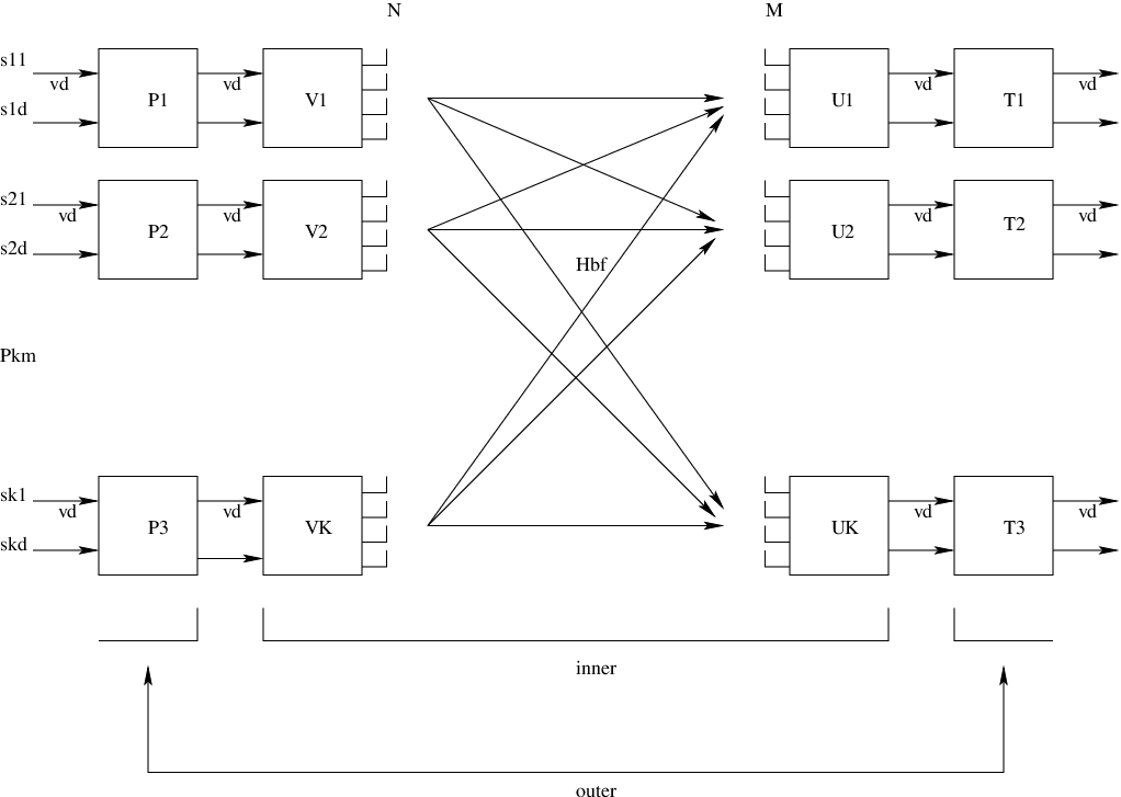
The optimal solution (23) has an interesting precoding and decoding structure, as shown in Fig. 2. That is, as noted previously, optimal linear processing under interference alignment is composed of two layers: inner precoders and decoders implement interference alignment to yield an other-user-interference-free single user channel for each transmit-receive pair, and outer precoders and decoders perform single-user optimal channel diagonalization for the single user channel resulting from the inner processing.

IV Properties of the Sum-Rate Based Algorithms and their Relationship with the Two-Layer Beamformer Structure

In this section, we investigate the properties and solution structure of the sum-rate-based beamformer design algorithms in Section II-A2, and establish an optimality of the max-SINR algorithm and the relationship between the sum-rate based algorithms and the two-layer linear beamformer of the previous section at high SNR. Under an assumption of sufficiently high SNR, we can use equal power distribution $P_{k}^{(m)}=P_{t}/Kd$ . We begin with an invariance property of the max-SINR algorithm for interference-aligning subspace, given in the following theorem.

Theorem 1

Any interference-aligning subspace is invariant under one composite iteration (composed of one VU step and one UV step) of the max-SINR algorithm at sufficiently high SNR. That is, when a set of interference-aligning beamforming matrices $\{{\bf V}_{k},{\bf U}_{k}\}$ are input to the iteration of the max-SINR algorithm, the resulting matrices after iteration have the same subspace and thus maintains the interference alignment property at sufficiently high SNR.

Proof: Let any interference-aligning beamforming matrices ${\bf V}_{k}=[{{\bf v}}_{k}^{(1)},{{\bf v}}_{k}^{(2)},\cdots,{{\bf v}}_{k}^{(d)}]$ and ${{\bf U}}_{k}=[{{\bf u}}_{k}^{(1)},{{\bf u}}_{k}^{(2)},\cdots,{{\bf u}}_{k}^{(d)}]$ be the input to the max-SINR algorithm at step $n$ (i.e., ${\bf V}_{k}[n]={{\bf V}}_{k}$ and ${\bf U}_{k}[n-1]={{\bf U}}_{k}$ for all $k$ ). For the $m$ -th stream of user $k$ , the receive filter is obtained by the max-SINR algorithm as

$\displaystyle{\mathbf{u}}_{k}^{(m)}[n]$	$\displaystyle=$	$\displaystyle{({\mathbf{R}}_{k}^{(m)}[n])^{-1}{\mathbf{H}}_{kk}{\mathbf{v}}_{k}^{(m)}[n]}\big/{\\|({\mathbf{R}}_{k}^{(m)}[n])^{-1}{\mathbf{H}}_{kk}{\mathbf{v}}_{k}^{(m)}[n]\\|},$	(42)
	$\displaystyle=$	$\displaystyle\left(\sum_{l\neq k}\frac{P_{t}}{Kd}{\bf H}_{kl}{{\bf V}}_{l}{{\bf V}}_{l}^{H}{\bf H}_{kl}^{H}+\sum_{j\neq m}\frac{P_{t}}{Kd}{\bf H}_{kk}{{\bf v}}_{k}^{(j)}{{\bf v}}_{k}^{(j)H}{\bf H}_{kk}^{H}+{\bf I}\right)^{-1}{\bf H}_{kk}{{\bf v}}_{k}^{(m)}\bigg/{\\|\cdot\\|},$
	$\displaystyle\stackrel{{\scriptstyle(a)}}{{=}}$	$\displaystyle\left(\left[{\bf q}_{k,m}^{(1)}\ {\bf q}_{k,m}^{(2)}\ \cdots\ {\bf q}_{k,m}^{(M)}\right]\left[\begin{array}[]{cccc}\lambda_{k,m}^{(1)}+1&\cdots&0&0\\ \vdots&\ddots&0&0\\ 0&0&\lambda_{k,m}^{(M-1)}+1&0\\ 0&0&0&1\\ \end{array}\right]\left[\begin{array}[]{c}{\bf q}_{k,m}^{(1)H}\\ {\bf q}_{k,m}^{(2)H}\\ \vdots\\ {\bf q}_{k,m}^{(M)H}\end{array}\right]\right)^{-1}{\bf H}_{kk}{{\bf v}}_{k}^{(m)}\big/\\|\cdot\\|,$
	$\displaystyle\stackrel{{\scriptstyle(b)}}{{=}}$	$\displaystyle{\bf q}_{k,m}^{(M)}{\bf q}_{k,m}^{(M)H}{\bf H}_{kk}{{\bf v}}_{k}^{(m)}\bigg/\\|\cdot\\|,~~~\mbox{as $P_{t}\rightarrow\infty$, i.e., for sufficiently high SNR},$
	$\displaystyle=$	$\displaystyle{\bf q}_{k,m}^{(M)}r_{k,m}e^{j\omega_{k,m}}\big/\\|\cdot\\|~~~\mbox{for a scalar $r_{k,m}e^{j\omega_{k,m}}={\bf q}_{k,m}^{(M)H}{\bf H}_{kk}{{\bf v}}_{k}^{(m)}$},$
	$\displaystyle=$	$\displaystyle{\bf q}_{k,m}^{(M)}e^{j\omega_{k,m}}.$

Equality (a) is because $\{{{\bf V}}_{k}\}$ satisfy the interference alignment condition, resulting in $\mbox{rank}(\sum_{l\neq k}$ ${\bf H}_{kl}{{\bf V}}_{l}{{\bf V}}_{l}^{H}{\bf H}_{kl}^{H})=d=M/2$ (see (6)), and the covariance matrix of the additional inter-stream interference has rank $d-1$ . Thus, the total rank is $M-1$ . Equality (b) is by the assumption of sufficiently high SNR. Collecting all $m=1,2,\cdots,d$ , the VU step of the max-SINR algorithm yields the receive beamforming matrix for user $k$ as

{\bf U}_{k}[n]=[{\bf q}_{k,1}^{(M)}e^{j\omega_{k,1}},\ {\bf q}_{k,2}^{(M)}e^{j\omega_{k,2}},\ \cdots,{\bf q}_{k,d}^{(M)}e^{j\omega_{k,d}}].

(43)

With this ${\bf U}_{k}[n]$ as the input to the UV step of the iteration, we obtain a new transmit beamforming matrix ${\bf V}_{k}[n+1]$ . For the $m$ -th stream of user $k$ ,

$\displaystyle{\mathbf{v}}_{k}^{(m)}[n+1]$	$\displaystyle=$	$\displaystyle{(\overleftarrow{{\mathbf{R}}}_{k}^{(m)}[n])^{-1}\overleftarrow{{\mathbf{H}}}_{kk}{\mathbf{u}}_{k}^{(m)}[n]}\big/{\\|(\overleftarrow{{\mathbf{R}}}_{k}^{(m)}[n])^{-1}\overleftarrow{{\mathbf{H}}}_{kk}{\mathbf{u}}_{k}^{(m)}[n]\\|}$	(53)
	$\displaystyle=$	$\displaystyle\left(\sum_{l\neq k}\frac{P_{t}}{Kd}\overleftarrow{{\bf H}}_{kl}{\bf U}_{l}[n]{\bf U}_{l}[n]^{H}\overleftarrow{{\bf H}}_{kl}^{H}+\sum_{j\neq m}\frac{P_{t}}{Kd}\overleftarrow{{\bf H}}_{kk}{\bf u}_{k}^{(j)}[n]{\bf u}_{k}^{(j)}[n]^{H}\overleftarrow{{\bf H}}_{kk}^{H}+{\bf I}\right)^{-1}\overleftarrow{{\bf H}}_{kk}{\bf u}_{k}^{(m)}[n]\bigg/{\\|\cdot\\|}$
	$\displaystyle\stackrel{{\scriptstyle(a)}}{{=}}$	$\displaystyle\left(\left[{\bf w}_{k,m}^{(1)}\ {\bf w}_{k,m}^{(2)}\ \cdots\ {\bf w}_{k,m}^{(M)}\right]\left[\begin{array}[]{cccc}\sigma_{k,m}^{(1)}+1&\cdots&0&0\\ \vdots&\ddots&0&0\\ 0&0&\sigma_{k,m}^{(M-1)}+1&0\\ 0&0&0&1\\ \end{array}\right]\left[\begin{array}[]{c}{\bf w}_{k,m}^{(1)H}\\ {\bf w}_{k,m}^{(2)H}\\ \vdots\\ {\bf w}_{k,m}^{(M)H}\end{array}\right]\right)^{-1}\overleftarrow{{\bf H}}_{kk}{\bf u}_{k}^{(m)}[n]\big/\\|\cdot\\|$
	$\displaystyle=$	$\displaystyle{\bf w}_{k,m}^{(M)}{\bf w}_{k,m}^{(M)H}\overleftarrow{{\bf H}}_{kk}{\bf u}_{k}^{(M)}[n]\bigg/\\|\cdot\\|,~~\mbox{as $P_{t}\rightarrow\infty$, i.e., for sufficiently high SNR,}~$
	$\displaystyle=$	$\displaystyle{\bf w}_{k,m}^{(M)}r^{\prime}_{k,m}e^{j\varphi_{k,m}}\big/\\|\cdot\\|~~~\mbox{for scalar $r^{\prime}_{k,m}e^{j\varphi_{k,m}}={\bf w}_{k,m}^{(M)H}\overleftarrow{{\bf H}}_{kk}{\bf u}_{k}^{(m)}[n]$}$
	$\displaystyle=$	$\displaystyle{\bf w}_{k,m}^{(M)}e^{j\varphi_{k,m}},$

where equality (a) is by Lemma 1, i.e., ${\cal C}({\bf U}_{k}[n])={\cal C}({{\bf U}}_{k})$ ( ${\bf U}_{k}[n]$ is also interference-aligning); thus, $\mbox{rank}(\overleftarrow{{{\bf Z}}}_{k})=d=M/2$ and $\overleftarrow{{\mathbf{R}}}_{k}^{(m)}[n]$ has rank $M-1$ in total, where

\overleftarrow{{{\bf Z}}}_{k}=\frac{P_{t}}{Kd}\sum_{l\neq k}\overleftarrow{{\bf H}}_{kl}{\bf U}_{l}[n]{\bf U}_{l}[n]^{H}\overleftarrow{{\bf H}}_{kl}^{H}.

(54)

The filters for other streams can be obtained similarly. Combining the filters for all streams of user $k$ , we have

{\bf V}_{k}[n+1]=[{\bf w}_{k,1}^{(M)}e^{j\varphi_{k,1}},\ {\bf w}_{k,2}^{(M)}e^{j\varphi_{k,2}},\ \cdots,\ {\bf w}_{k,d}^{(M)}e^{j\varphi_{k,d}}].

(55)

By similar argument as in Lemma 1, we have

{\cal C}({\bf V}_{k}[n+1])={\cal C}([{\bf w}_{k,1}^{(M)},\ \cdots,{\bf w}_{k,d}^{(M)}])={\cal C}(\overleftarrow{{{\bf Z}}}_{k})^{\bot}={\cal C}({{\bf V}}_{k}).

(56)

Thus, we have

{\cal C}({\bf V}_{k}[n+1])={\cal C}({{\bf V}}_{k})={\cal C}({\bf V}_{k}[n]).

(57)

That is, one composite iteration of the max-SINR algorithm preserves an interference-aligning subspace at sufficiently high SNR.

Lemma 1

For the ${\bf U}_{k}[n]$ in (43) obtained by the VU step of the max-SINR iteration, the following holds:

{\cal C}({\bf U}_{k}[n])={\mathcal{C}}([{\bf q}_{k,1}^{(M)},\ {\bf q}_{k,2}^{(M)},\ \cdots,{\bf q}_{k,d}^{(M)}])\subset{\mathcal{C}}({{\bf Z}}_{k})^{\bot}={\mathcal{C}}({{\bf U}}_{k})

(58)

where ${{\bf Z}}_{k}=\frac{P_{t}}{Kd}\sum_{l\neq k}{\bf H}_{kl}{{\bf V}}_{l}{{\bf V}}_{l}^{H}{\bf H}_{kl}^{H}$ . When the rank of ${\bf U}_{k}[n]$ is $d$ ,

{\mathcal{C}}({\bf U}_{k}[n])={\mathcal{C}}([{\bf q}_{k,1}^{(M)},\ {\bf q}_{k,2}^{(M)},\ \cdots,\ {\bf q}_{k,d}^{(M)}])={\mathcal{C}}({{\bf Z}}_{k})^{\bot}={\mathcal{C}}({{\bf U}}_{k}).

(59)

Proof: Let the SVD of ${{\bf Z}}_{k}$ be

{{\bf Z}}_{k}=\left[{\bf z}_{k}^{(1)}\ {\bf z}_{k}^{(2)}\ \cdots{\bf z}_{k}^{(M)}\right]\left[\begin{array}[]{lc}\hbox{$\bf\Sigma$}_{k}&{\mathbf{0}}_{d\times d}\\ {\mathbf{0}}_{d\times d}&{\mathbf{0}}_{d\times d}\end{array}\right]\left[\begin{array}[]{c}{\bf z}_{k}^{(1)H}\\ {\bf z}_{k}^{(2)H}\\ \vdots\\ {\bf z}_{k}^{(M)H}\end{array}\right],

(60)

where $\hbox{$\bf\Sigma$}_{k}$ is a $d\times d$ diagonal matrix containing non-zero singular values of ${{\bf Z}}_{k}$ . (This is because $\{{{\bf V}}_{k}\}$ is interference-aligning.) Hence,

{\cal C}({{\bf Z}}_{k})^{\bot}={\cal C}([{\bf z}_{k}^{(d+1)},\cdots,{\bf z}_{k}^{(M)}])={\cal C}({\bf U}_{k}).

(61)

Furthermore, we can see from (IV) that

{\bf q}_{k,m}^{(M)}={\cal C}([{\bf q}_{k,m}^{(1)},{\bf q}_{k,m}^{(2)},\cdots,{\bf q}_{k,m}^{(M-1)}])^{\bot}\quad\mbox{for all~ }m,

(62)

and for all $m$

{\mathcal{C}}({{\bf Z}}_{k})\subset{\mathcal{C}}({{\bf R}}_{k}^{(m)}[n])={\mathcal{C}}([{\bf q}_{k,m}^{(1)},{\bf q}_{k,m}^{(2)},\cdots,{\bf q}_{k,m}^{(M-1)}])

(63)

since ${\bf Z}_{k}$ is contained in ${\bf R}_{k}^{(m)}$ . Now, (62) and (63) imply

{\bf q}_{k,m}^{(M)}={\mathcal{C}}([{\bf q}_{k,m}^{(1)},\cdots,{\bf q}_{k,m}^{(M-1)}])^{\bot}\subset{\mathcal{C}}({{\bf Z}}_{k})^{\bot},

(64)

since ${\mathcal{C}}({\bf A})\subset{\mathcal{C}}({\bf B})$ $\Rightarrow$ ${\mathcal{C}}({\bf B})^{\bot}\subset{\mathcal{C}}({\bf A})^{\bot}$ . Since ${\bf q}_{k,m}^{(M)}\in{\mathcal{C}}({{\bf Z}}_{k})^{\bot}$ for each $m\in\{1,2,\cdots,d\}$ , we have

{\mathcal{C}}([{\bf q}_{k,1}^{(M)},{\bf q}_{k,2}^{(M)},\cdots,{\bf q}_{k,d}^{(M)}])\subset{\mathcal{C}}({{\bf Z}}_{k})^{\bot},

(65)

and (58) follows from (61) and (65). When $\mbox{rank}([{\bf q}_{k,m}^{(1)},{\bf q}_{k,m}^{(2)},\cdots,{\bf q}_{k,m}^{(d)}])=d=\mbox{rank}({{\bf Z}}_{k})$ , two subspaces are the same, i.e.,

{\mathcal{C}}([{\bf q}_{k,1}^{(M)},{\bf q}_{k,2}^{(M)},\cdots,{\bf q}_{k,d}^{(M)}])={\mathcal{C}}({{\bf Z}}_{k})^{\bot}={\cal C}({\bf U}_{k}).

(66)

Next, we investigate the fixed point structure of the max-SINR algorithm by showing the relationship between the (coder) optimal two-layer precoder and decoder structure in Section III and the max-SINR algorithm.

Theorem 2

The two-layer linear beamforming solution (23) with optimal outer coder under interference alignment, i.e., $\{{\bf V}_{k}^{*}=\underline{{\bf V}}_{k}\mbox{${\bf\Phi}$}_{k}^{*}(\{\underline{{\bf V}}_{k},\underline{{\bf U}}_{k}\}),{\bf U}_{k}^{*}=\underline{{\bf U}}_{k}\hbox{$\bf\Theta$}_{k}^{*}(\{\underline{{\bf V}}_{k},\underline{{\bf U}}_{k}\})$ , is a fixed point of the max-SINR algorithm for any interference-aligning matrices $\{\underline{{\bf V}}_{k},\underline{{\bf U}}_{k}\}$ at sufficiently high SNR.

Proof: Set $\{{\bf V}_{k}^{*}=\underline{{\bf V}}_{k}\mbox{${\bf\Phi}$}_{k}^{*}\}$ as the input to the VU step of the max-SINR iteration. Let ${\bf U}_{k}[n]=[{\bf q}_{k,1}^{(M)}e^{j\omega_{k,1}},\cdots,$ ${\bf q}_{k,d}^{(M)}e^{j\omega_{k,d}}]$ of (43) be the corresponding output of the VU step (the notation here follows Theorem 1). From (IV), ${\bf q}_{k,m}^{(M)}\ \bot\ {\mathcal{C}}([{\bf q}_{k,m}^{(1)},{\bf q}_{k,m}^{(2)},\cdots,{\bf q}_{k,m}^{(M-1)}])={\cal C}({\bf R}_{k}^{(m)})$ and this implies

	$\displaystyle 0$	$\displaystyle=$	$\displaystyle{\bf q}_{k,m}^{(M)H}\left(\sum_{l\neq k}{\bf H}_{kl}{\bf V}^{}_{l}{\bf V}^{H}_{l}{\bf H}_{kl}^{H}+\sum_{j\neq m}{\bf H}_{kk}{\bf v}_{k}^{(j)}{\bf v}_{k}^{(j)H}{\bf H}_{kk}^{H}\right){\bf q}_{k,m}^{(M)}$		(67)
		$\displaystyle=$	$\displaystyle{\bf q}_{k,m}^{(M)H}\left(\sum_{l\neq k}{\bf H}_{kl}{\bf V}^{}_{l}{\bf V}^{H}_{l}{\bf H}_{kl}^{H}\right){\bf q}_{k,m}^{(M)}+{\bf q}_{k,m}^{(M)H}\left(\sum_{j\neq m}{\bf H}_{kk}{\bf v}_{k}^{(j)}{\bf v}_{k}^{(j)H}{\bf H}_{kk}^{H}\right){\bf q}_{k,m}^{(M)}.$		(68)

From Lemma 1 we have

{\mathcal{C}}([{\bf q}_{k,1}^{(M)},\ {\bf q}_{k,2}^{(M)},\ \cdots,\ {\bf q}_{k,d}^{(M)}])\subset{\mathcal{C}}({\bf U}_{k}^{*})={\mathcal{C}}(\underline{{\bf U}}_{k}).

(69)

Because of this, the first term on the RHS in (68) is nulled out by the interference alignment condition. Also, (69) implies that for each $m$

{\bf q}_{k,m}^{(M)}=\underline{{\bf U}}_{k}{\bf x}_{km}

(70)

for some vector ${\bf x}_{km}$ . Denote ${\bf V}_{k}^{*}$ as

{\bf V}_{k}^{*}=[{\bf v}_{k}^{*(1)},~{\bf v}_{k}^{*(2)},\cdots,~{\bf v}_{k}^{*(d)}]=\underline{{\bf V}}_{k}\mbox{${\bf\Phi}$}_{k}^{*}=\underline{{\bf V}}_{k}[\hbox{\boldmath$\phi$\unboldmath}_{k}^{*(1)},\hbox{\boldmath$\phi$\unboldmath}_{k}^{*(2)},\cdots,\hbox{\boldmath$\phi$\unboldmath}_{k}^{*(d)}],

(71)

where $\mbox{${\bf\Phi}$}_{k}^{*}$ is a unitary matrix composed of the right singular vectors of the single-user equivalent channel $\bar{{\bf H}}_{k}=\underline{{\bf U}}_{k}^{H}{\bf H}_{kk}\underline{{\bf V}}_{k}$ in (28) with SVD $\bar{{\bf H}}_{k}=\bar{{\bf U}}_{k}\bar{\mbox{$\bf\Lambda$}}_{k}\bar{{\bf V}}_{k}^{H}=\hbox{$\bf\Theta$}_{k}^{*}\bar{\mbox{$\bf\Lambda$}}_{k}\mbox{${\bf\Phi}$}^{*H}_{k}$ (see (31)). Since both terms of the RHS of (68) are nonnegative, we have for the second term

$\displaystyle 0$	$\displaystyle=$	$\displaystyle\textstyle{\bf q}_{k,m}^{(M)H}(\sum_{j\neq m}{\bf H}_{kk}{\bf v}_{k}^{(j)}{\bf v}_{k}^{(j)H}{\bf H}_{kk}^{H}){\bf q}_{k,m}^{(M)},$	(72)
	$\displaystyle=$	$\displaystyle\textstyle\sum_{j\neq m}{\bf q}_{k,m}^{(M)H}{\bf H}_{kk}{\bf v}_{k}^{(j)}{\bf v}_{k}^{(j)H}{\bf H}_{kk}^{H}{\bf q}_{k,m}^{(M)},$
	$\displaystyle=$	$\displaystyle\textstyle\sum_{j\neq m}\left\|{\bf q}_{k,m}^{(M)H}{\bf H}_{kk}{\bf v}_{k}^{*(j)}\right\|^{2},$
	$\displaystyle\stackrel{{\scriptstyle(a)}}{{=}}$	$\displaystyle\textstyle\sum_{j\neq m}\left\|{\bf x}_{km}^{H}\underline{{\bf U}}_{k}^{H}{\bf H}_{kk}\underline{{\bf V}}_{k}\hbox{\boldmath$\phi$\unboldmath}_{k}^{*(j)}\right\|^{2},$
	$\displaystyle\stackrel{{\scriptstyle(b)}}{{=}}$	$\displaystyle\textstyle\sum_{j\neq m}\left\|{\bf x}_{km}^{H}\bar{{\bf H}}_{k}\hbox{\boldmath$\phi$\unboldmath}_{k}^{*(j)}\right\|^{2},$
	$\displaystyle\stackrel{{\scriptstyle(c)}}{{=}}$	$\displaystyle\textstyle\sum_{j\neq m}\left\|{\bf x}_{km}^{H}(\hbox{$\bf\Theta$}_{k}^{}\bar{\mbox{$\bf\Lambda$}}_{k}\mbox{${\bf\Phi}$}^{H}_{k})\hbox{\boldmath$\phi$\unboldmath}_{k}^{*(j)}\right\|^{2},$
	$\displaystyle=$	$\displaystyle\textstyle\sum_{j\neq m}\left\|{\bf x}_{km}^{H}(\sum_{i=1}^{d}\bar{\lambda}_{k}^{(i)}{\mbox{\boldmath$\theta$\unboldmath}}_{k}^{(i)}\hbox{\boldmath$\phi$\unboldmath}_{k}^{(i)H})\hbox{\boldmath$\phi$\unboldmath}_{k}^{*(j)}\right\|^{2},$
	$\displaystyle\stackrel{{\scriptstyle(d)}}{{=}}$	$\displaystyle\textstyle\sum_{j\neq m}\left\|{\bf x}_{km}^{H}(\bar{\lambda}_{k}^{(j)}{\mbox{\boldmath$\theta$\unboldmath}}_{k}^{*(j)})\right\|^{2},$
	$\displaystyle=$	$\displaystyle\textstyle\sum_{j\neq m}\left\|\bar{\lambda}_{k}^{(j)}{\bf x}_{km}^{H}{\mbox{\boldmath$\theta$\unboldmath}}_{k}^{*(j)}\right\|^{2},$

where (a) is by (70) and (71), (b) is by the definition of the equivalent channel, (c) is by its SVD and (d) is because $\mbox{${\bf\Phi}$}_{k}^{*}$ is unitary. Since each term in the summation in (72) is non-negative, each term (i.e., for each $j$ ) is zero for the sum to be zero. Therefore, the unique ${\bf x}_{km}$ satisfying this is given by

{\bf x}_{km}={\mbox{\boldmath$\theta$\unboldmath}}_{k}^{*(m)}

(73)

since $\hbox{$\bf\Theta$}_{k}^{*}$ is unitary, and thus

{\bf q}_{k,m}^{(M)}=\underline{{\bf U}}_{k}{\mbox{\boldmath$\theta$\unboldmath}}_{k}^{*(m)}.

(74)

The filters for other streams can be obtained similarly. Combining all the streams yields

$\displaystyle{\bf U}_{k}[n]$	$\displaystyle=$	$\displaystyle[{\bf q}_{k,1}^{(M)}e^{j\omega_{k,1}},\ {\bf q}_{k,2}^{(M)}e^{j\omega_{k,2}},\ \cdots,\ {\bf q}_{k,d}^{(M)}e^{j\omega_{k,d}}],$	(75)
	$\displaystyle=$	$\displaystyle[\underline{{\bf U}}_{k}{\mbox{\boldmath$\theta$\unboldmath}}_{k}^{(1)}e^{j\omega_{k,1}},\ \underline{{\bf U}}_{k}{\mbox{\boldmath$\theta$\unboldmath}}_{k}^{(2)}e^{j\omega_{k,2}},\ \cdots,\ \underline{{\bf U}}_{k}{\mbox{\boldmath$\theta$\unboldmath}}_{k}^{*(d)}e^{j\omega_{k,d}}],$	(76)
	$\displaystyle=$	$\displaystyle\underline{{\bf U}}_{k}\hbox{$\bf\Theta$}_{k}^{*}\mbox{diag}(e^{j\omega_{k,1}},e^{j\omega_{k,2}},\cdots,e^{j\omega_{k,d}}),$	(77)
	$\displaystyle=$	$\displaystyle[{\bf u}_{k}^{(1)}e^{j\omega_{k,1}},\ {\bf u}_{k}^{(2)}e^{j\omega_{k,2}},\ \cdots,~{\bf u}_{k}^{*(d)}e^{j\omega_{k,d}}].$	(78)

This is valid for all $k$ (i.e., for all users).

Now consider the UV step of the iteration from ${\bf U}_{k}[n]={\bf U}_{k}^{*}\mbox{diag}(e^{j\omega_{k,1}},\cdots,e^{j\omega_{k,d}})$ to ${\bf V}_{k}[n+1]$ . From (55) in the proof of Theorem 1, we have

{\bf V}_{k}[n+1]=[{\bf w}_{k,1}^{(M)}e^{j\varphi_{k,1}},\ {\bf w}_{k,2}^{(M)}e^{j\varphi_{k,2}},\ \cdots,\ {\bf w}_{k,d}^{(M)}e^{j\varphi_{k,d}}]

and (IV) shows that ${\bf w}_{k,m}^{(M)}\ \bot\ {\mathcal{C}}([{\bf w}_{k,m}^{(1)},{\bf w}_{k,m}^{(2)},\cdots,{\bf w}_{k,m}^{(M-1)}])={\cal C}(\overleftarrow{{\bf R}}_{k}^{(m)})$ . From this and (IV) we have

	$\displaystyle 0$	$\displaystyle=$	$\displaystyle{\bf w}_{k,m}^{(M)H}\left(\sum_{l\neq k}\overleftarrow{{\bf H}}_{kl}{{\bf U}}_{l}[n]{{\bf U}}_{l}^{H}[n]\overleftarrow{{\bf H}}_{kl}^{H}+\sum_{j\neq m}\overleftarrow{{\bf H}}_{kk}{\bf u}_{k}^{(j)}[n]({\bf u}_{k}^{(j)}[n])^{H}\overleftarrow{{\bf H}}_{kk}^{H}\right){\bf w}_{k,m}^{(M)}$		(79)
		$\displaystyle=$	$\displaystyle{\bf w}_{k,m}^{(M)H}\left(\sum_{l\neq k}\overleftarrow{{\bf H}}_{kl}{{\bf U}}^{}_{l}{{\bf U}}^{H}_{l}\overleftarrow{{\bf H}}_{kl}^{H}\right){\bf w}_{k,m}^{(M)}+{\bf w}_{k,m}^{(M)H}\left(\sum_{j\neq m}\overleftarrow{{\bf H}}_{kk}{\bf u}_{k}^{(j)}{\bf u}_{k}^{(j)H}\ \overleftarrow{{\bf H}}_{kk}^{H}\right){\bf w}_{k,m}^{(M)}.$		(80)

By (56) we have

{\cal C}([{\bf w}_{k,1}^{(M)},{\bf w}_{k,2}^{(M)},\cdots,{\bf w}_{k,d}^{(M)}])\subset{\cal C}({\bf V}_{k}^{*})={\cal C}(\overleftarrow{{\bf Z}}_{k}^{*})^{\perp},

(81)

where $\overleftarrow{{\bf Z}}_{k}^{*}=(P_{t}/Kd)\sum_{l\neq k}\overleftarrow{{\bf H}}_{kl}{{\bf U}}_{l}^{*}{{\bf U}}_{l}^{*H}\overleftarrow{{\bf H}}_{kl}^{H}$ . This implies that the first term on the RHS of (80) is zero and for each $m$

{\bf w}_{k,m}^{(M)}=\underline{{\bf V}}_{k}{\bf y}_{km}

for some vector ${\bf y}_{km}$ . By a procedure similar to that used to obtain (73) we obtain the unique ${\bf y}_{km}=\hbox{\boldmath$\phi$\unboldmath}_{k}^{*(m)}$ . Hence, ${\bf w}_{k,m}^{(M)}=\underline{{\bf V}}_{k}\hbox{\boldmath$\phi$\unboldmath}_{k}^{*(m)}$ . Combining all the streams yields,

$\displaystyle{\bf V}_{k}[n+1]$	$\displaystyle=$	$\displaystyle[{\bf w}_{k,1}^{(M)}e^{j\varphi_{k,1}},\ {\bf w}_{k,2}^{(M)}e^{j\varphi_{k,2}},\ \cdots,\ {\bf w}_{k,d}^{(M)}e^{j\varphi_{k,d}}],$	(82)
	$\displaystyle=$	$\displaystyle[\underline{{\bf V}}_{k}\hbox{\boldmath$\phi$\unboldmath}_{k}^{(1)}e^{j\varphi_{k,1}},\ \underline{{\bf V}}_{k}\hbox{\boldmath$\phi$\unboldmath}_{k}^{(2)}e^{j\varphi_{k,2}},\ \cdots,\ \underline{{\bf V}}_{k}\hbox{\boldmath$\phi$\unboldmath}_{k}^{*(d)}e^{j\varphi_{k,d}}],$	(83)
	$\displaystyle=$	$\displaystyle\underline{{\bf V}}_{k}\mbox{${\bf\Phi}$}_{k}^{*}\mbox{diag}(e^{j\varphi_{k,1}},e^{j\varphi_{k,2}},\cdots,e^{j\varphi_{k,d}}),$	(84)
	$\displaystyle=$	$\displaystyle[{\bf v}_{k}^{(1)}e^{j\varphi_{k,1}},\ {\bf v}_{k}^{(2)}e^{j\varphi_{k,2}},\ \cdots,~{\bf v}_{k}^{*(d)}e^{j\varphi_{k,d}}]$	(85)

for all $k$ . Now, recall from (53) that $r^{\prime}_{k,m}e^{j\varphi_{k,m}}={\bf w}_{k,m}^{(M)H}\overleftarrow{{\bf H}}_{kk}{\bf u}_{k}^{(m)}[n]$ . Substituting ${\bf w}_{k,m}^{(M)}={\bf v}_{k}^{*(m)}$ and ${\bf u}_{k}^{(m)}[n]={\bf u}_{k}^{*(m)}e^{j\omega_{k,m}}$ into (53) yields

r^{\prime}_{k,m}e^{j\varphi_{k,m}}={\bf w}_{k,m}^{(M)H}\overleftarrow{{\bf H}}_{kk}{\bf u}_{k}^{(m)}[n]={\bf v}_{k}^{*(m)H}\overleftarrow{{\bf H}}_{kk}{\bf u}_{k}^{*(m)}e^{j\omega_{k,m}}.

(86)

Also, substituting ${\bf q}_{k,m}^{(M)}$ in (42) with (74) yields

r_{k,m}e^{j\omega_{k,m}}={\bf q}_{k,m}^{(M)H}{\bf H}_{kk}{\bf v}_{k}^{*(m)}={\bf u}_{k}^{*(m)H}{\bf H}_{kk}{\bf v}_{k}^{*(m)}.

(87)

From (86) and (87) we have

r^{\prime}_{k,m}e^{j\varphi_{k,m}}={\bf v}_{k}^{*(m)H}\overleftarrow{{\bf H}}_{kk}{\bf u}_{k}^{*(m)}e^{j\omega_{k,m}}=r_{k,m}e^{-j\omega_{k,m}}e^{j\omega_{k,m}}=r_{k,m},

(88)

and thus $\varphi_{k,m}=0$ since both $r_{k,m}$ and $r^{\prime}_{k,m}$ are real. This holds for all streams and users, i.e., $\varphi_{k,m}=0$ for all $k$ and $m$ . Finally, from (82) and $\varphi_{k,m}=0$ , we have

{\bf V}_{k}[n+1]={\bf V}_{k}^{*}={\bf V}_{k}[n].

(89)

Thus, the two-layer linear beamforming solution $\{\underline{{\bf V}}_{k}\mbox{${\bf\Phi}$}_{k}^{*},\underline{{\bf U}}_{k}\hbox{$\bf\Theta$}_{k}^{*}\}$ is a fixed point of the max-SINR algorithm at sufficiently high SNR.

Note that if the outer precoder and decoder ${\bf\Phi}$ and $\bf\Theta$ are not optimized to the single user equivalent channel $\bar{{\bf H}}_{k}$ resulting from interference alignment by the inner precoder and decoder $\{\underline{{\bf V}}_{k},\underline{{\bf U}}_{k}\}$ , then (73) and (74) are not valid and thus the beamforming matrices change with the iteration; the interference-aligning solution with suboptimal outer coders (including the zero-forcing $\hbox{$\bf\Theta$}_{k}=(\bar{{\bf H}}_{k}\mbox{${\bf\Phi}$})^{\dagger}$ ) within the given space is not a fixed point of the max-SINR algorithm. (Numerical result confirming this will be shown in Section V.) Now define the optimal interference-aligning subspaces as the column spaces of matrices

\{\underline{{\bf V}}_{k}^{*},\underline{{\bf U}}_{k}^{*}\}=\mathop{\arg\max}_{\underline{{\bf V}}_{k},\underline{{\bf U}}_{k}}R(\underline{{\bf V}}_{k}\mbox{${\bf\Phi}$}_{k}^{*}(\{\underline{{\bf V}}_{k},\underline{{\bf U}}_{k}\}),\underline{{\bf U}}_{k}\hbox{$\bf\Theta$}_{k}^{*}(\{\underline{{\bf V}}_{k},\underline{{\bf U}}_{k}\})),

(90)

which achieves $R_{IA}^{*}$ . Then, since Theorem 2 is valid for any interference-aligning matrices, we have the following corollary to Theorem 2.

Corollary 1

$\{{\bf V}_{k}^{**}=\underline{{\bf V}}_{k}^{*}\mbox{${\bf\Phi}$}^{*}(\underline{{\bf V}}_{k}^{*},\underline{{\bf U}}_{k}^{*}),{\bf U}_{k}^{**}=\underline{{\bf U}}_{k}^{*}\hbox{$\bf\Theta$}^{*}(\underline{{\bf V}}_{k}^{*},\underline{{\bf U}}_{k}^{*})\}$ is a fixed point of the max-SINR algorithm at sufficiently high SNR.

Lemma 2

The globally optimal fixed point of the max-SINR algorithm (in the sense that it has the maximum sum rate among all its fixed points) satisfies the interference alignment condition at sufficiently high SNR.

Proof: Suppose that the globally optimal fixed point does not satisfy the interference alignment condition. Then, due to the interference leakage the SINR of a certain stream does not increase unboundedly as the signal power tends to infinity and the maximum number of degrees of freedom is not achieved with this assumed ”globally optimal” fixed point. Therefore, this assumed globally optimal fixed point has lower sum rate than the interference-aligning fixed point $\{{\bf V}_{k}^{**},{\bf U}_{k}^{**}\}$ in Corollary 1 at sufficiently high SNR, and it is not globally optimal among the fixed points of the max-SINR algorithm. Thus, we have a contradiction, and hence the claim follows.

Theorem 3

$\{{\bf V}_{k}^{**},{\bf U}_{k}^{**}\}$ in Corollary 1 is the globally optimal fixed point of the max-SINR algorithm at sufficiently high SNR.

Proof: By Lemma 2 the globally optimal fixed point of the max-SINR algorithm is interference-aligning at sufficiently high SNR. Among all interference-aligning beamforming matrices, $\{{\bf V}_{k}^{**},{\bf U}_{k}^{**}\}$ has the maximum sum rate $R_{IA}^{*}$ and it is also a fixed point of the max-SINR algorithm by Corollary 1. Hence, $\{{\bf V}_{k}^{**},{\bf U}_{k}^{**}\}$ is the globally optimal fixed-point of the max-SINR algorithm at sufficiently high SNR.

Theorem 3 established an optimality property for the max-SINR algorithm at high SNR. At high SNR one can deduce that the optimal beamformer among all linear beamformers should satisfy the interference alignment condition at high SNR by an argument similar to that used in Lemma 2 and thus $R_{IA}^{*}$ in (32) is the best sum rate achievable by linear processing at sufficiently high SNR. Thus, the max-SINR algorithm is optimal at high SNR among all linear beamformers in the sense that the set of its fixed points includes the globally optimal linear beamforming solution $\{{\bf V}_{k}^{**},{\bf U}_{k}^{**}\}$ . One algorithmic advantage of the max-SINR algorithm is that it updates the beamforming matrices at least to be outer-coder optimal. The benefit is evident when we consider the sum-rate gradient algorithm based on the user-by-user approach (2, 14, 19), which has a much larger set of fixed points as described in the following theorem.

Theorem 4

Any set $\{\check{{\bf V}}_{k},k=1,2,\cdots,K\}$ of interference-aligning beamforming matrices is a fixed point of the sum-rate gradient algorithm in Section II-A2 at sufficiently high SNR.

Proof: This result can be proven by computing the gradient (22) at $\{\check{{\bf V}}_{k}\}$ . The gradient (22) at $\{\check{{\bf V}}_{k}\}$ is given by

\nabla_{{\bf V}_{k}^{o}}C({\bf V}_{1},\cdots,{\bf V}_{K})|_{\check{{\bf V}}_{k}}=\sum_{l=1}^{K}\frac{P_{t}}{Kd}{\bf H}_{lk}^{H}{\bf R}_{l}^{-1}{\bf H}_{lk}\check{{\bf V}}_{k}-\sum_{l\neq k}\frac{P_{t}}{Kd}{\bf H}_{lk}^{H}({\bf I}+{\bf Z}_{l})^{-1}{\bf H}_{lk}\check{{\bf V}}_{k}.

(91)

The SVD of the term $({\bf I}+{\bf Z}_{l})^{-1}$ on the RHS of the above equation is obtained from (60) and is given by

	$\displaystyle({\bf I}+{\bf Z}_{l})^{-1}$	$\displaystyle=$	$\displaystyle\left[{\bf z}_{l}^{(1)}\ {\bf z}_{l}^{(2)}\ \cdots{\bf z}_{l}^{(M)}\right]\left[\begin{array}[]{cc}\hbox{$\bf\Sigma$}_{l}+{\bf I}_{d\times d}&{\mathbf{0}}_{d\times d}\\ {\mathbf{0}}_{d\times d}&{\bf I}_{d\times d}\end{array}\right]^{-1}\left[\begin{array}[]{c}{\bf z}_{l}^{(1)H}\\ {\bf z}_{l}^{(2)H}\\ \vdots\\ {\bf z}_{l}^{(M)H}\end{array}\right]$		(99)
		$\displaystyle=$	$\displaystyle\left[{\bf z}_{l}^{(d+1)}\ {\bf z}_{l}^{(d+2)}\ \cdots{\bf z}_{l}^{(M)}\right]\left[{\bf z}_{l}^{(d+1)}\ {\bf z}_{l}^{(d+2)}\ \cdots{\bf z}_{l}^{(M)}\right]^{H}$		(99)

as $P_{t}\rightarrow\infty$ since the nonzero singular values of ${\bf Z}_{l}$ increases without bound as $P_{t}\rightarrow\infty$ . From Lemma 1, we have ${\mathcal{C}}([{\bf z}_{l}^{(d+1)},\cdots,{\bf z}_{l}^{(M)}])={\cal C}({\bf Z}_{l})^{\perp}={\mathcal{C}}(\check{{\bf U}}_{l})$ . Due to the interference alignment by $\{\check{{\bf V}}_{k},\check{{\bf U}}_{k}\}$ , we have

({\bf I}+{\bf Z}_{l})^{-1}{\bf H}_{lk}\check{{\bf V}}_{k}={\mathbf{0}},

(100)

for $l\neq k$ , and thus the second term on the RHS of (91) vanishes at sufficiently high SNR. Now consider the first term on the RHS of (91). From the matrix inversion lemma, we have

	$\displaystyle{\bf R}_{l}^{-1}$	$\displaystyle=$	$\displaystyle\left({\bf I}+{\bf Z}_{l}+\frac{P_{t}}{Kd}{\bf H}_{ll}\check{{\bf V}}_{l}\check{{\bf V}}_{l}^{H}{\bf H}_{ll}^{H}\right)^{-1}=\left({\bf M}_{l}+\frac{P_{t}}{Kd}{\bf H}_{ll}\check{{\bf V}}_{l}\check{{\bf V}}_{l}^{H}{\bf H}_{ll}^{H}\right)^{-1}$		(101)
		$\displaystyle=$	$\displaystyle{\bf M}_{l}^{-1}-\frac{P_{t}}{Kd}{\bf M}_{l}^{-1}{\bf H}_{ll}\check{{\bf V}}_{l}\left({\bf I}+\frac{P_{t}}{Kd}\check{{\bf V}}_{l}^{H}{\bf H}_{ii}^{H}{\bf M}_{l}^{-1}{\bf H}_{ll}\check{{\bf V}}_{l}\right)^{-1}\check{{\bf V}}_{l}^{H}{\bf H}_{ll}^{H}{\bf M}_{l}^{-1},$		(101)

where ${\bf M}_{l}={\bf I}+{\bf Z}_{l}$ . Substituting this into the second term yields

			$\displaystyle\sum_{l=1}^{K}\frac{P_{t}}{Kd}{\bf H}_{lk}^{H}{\bf R}_{l}^{-1}{\bf H}_{lk}\check{{\bf V}}_{k}$		(102)
		$\displaystyle=$	$\displaystyle\sum_{l=1}^{K}\frac{P_{t}}{Kd}{\bf H}_{lk}^{H}\left({\bf M}_{l}^{-1}-\frac{P_{t}}{Kd}{\bf M}_{l}^{-1}{\bf H}_{ll}\check{{\bf V}}_{l}\left({\bf I}+\frac{P_{t}}{Kd}\check{{\bf V}}_{l}^{H}{\bf H}_{ll}^{H}{\bf M}_{l}^{-1}{\bf H}_{ll}\check{{\bf V}}_{l}\right)^{-1}\check{{\bf V}}_{l}^{H}{\bf H}_{ll}^{H}{\bf M}_{l}^{-1}\right){\bf H}_{lk}\check{{\bf V}}_{k}.$		(102)

Since ${\bf M}_{l}^{-1}{\bf H}_{lk}\check{{\bf V}}_{k}={\mathbf{0}}$ for all $l\neq k$ by (100), we have

	$\displaystyle\nabla_{{\bf V}_{k}^{o}}C({\bf V}_{1},\cdots,{\bf V}_{K})\|_{\check{{\bf V}}_{k}}=\frac{P_{t}}{Kd}{\bf H}_{kk}^{H}{\bf M}_{k}^{-1}{\bf H}_{kk}\check{{\bf V}}_{k}$	(103)
	$\displaystyle-\left(\frac{P_{t}}{Kd}\right)^{2}{\bf H}_{kk}^{H}{\bf M}_{k}^{-1}{\bf H}_{kk}\check{{\bf V}}_{k}\left({\bf I}+\frac{P_{t}}{Kd}\check{{\bf V}}_{k}^{H}{\bf H}_{kk}^{H}{\bf M}_{k}^{-1}{\bf H}_{kk}\check{{\bf V}}_{k}\right)^{-1}\check{{\bf V}}_{k}^{H}{\bf H}_{kk}^{H}{\bf M}_{k}^{-1}{\bf H}_{kk}\check{{\bf V}}_{k}+o(1)$
$\displaystyle\stackrel{{\scriptstyle(a)}}{{=}}$	$\displaystyle\frac{P_{t}}{Kd}{\bf H}_{kk}^{H}{\bf M}_{k}^{-1}{\bf H}_{kk}\check{{\bf V}}_{k}$
	$\displaystyle-\left(\frac{P_{t}}{Kd}\right)^{2}{\bf H}_{kk}^{H}{\bf M}_{k}^{-1}{\bf H}_{kk}\check{{\bf V}}_{k}\left(\frac{P_{t}}{Kd}\check{{\bf V}}_{k}^{H}{\bf H}_{kk}^{H}{\bf M}_{k}^{-1}{\bf H}_{kk}\check{{\bf V}}_{k}\right)^{-1}\check{{\bf V}}_{k}^{H}{\bf H}_{kk}^{H}{\bf M}_{k}^{-1}{\bf H}_{kk}\check{{\bf V}}_{k}+o(1)$
$\displaystyle=$	$\displaystyle\frac{P_{t}}{Kd}{\bf H}_{kk}^{H}{\bf M}_{k}^{-1}{\bf H}_{kk}\check{{\bf V}}_{k}-\frac{P_{t}}{Kd}{\bf H}_{kk}^{H}{\bf M}_{k}^{-1}{\bf H}_{kk}\check{{\bf V}}_{k}+o(1)$
$\displaystyle=$	$\displaystyle{\mathbf{0}}~~\mbox{as}~~P_{t}\rightarrow\infty,$

where (a) holds for sufficiently high SNR since ${\bf M}_{l}^{-1}$ in (99) does not depend on $P_{t}$ . Hence, the gradient is zero at $\{\check{{\bf V}}_{k}\}$ and $\{\check{{\bf V}}_{k}\}$ is a fixed point of the sum-rate gradient algorithm at sufficiently high SNR.

Now the difference between the stream-by-stream approach and the user-by-user approach is clear under equal power allocation to all streams. One could have conjectured that aggregating all the streams of a user together and formulating the sum rate problem correspondingly to construct an algorithm might yield better performance. However, there is an algorithmic disadvantage of such a formulation at least at high SNR. For the user-by-user approach (2, 14, 19) to algorithm construction, there is no resolving power of the algorithm to distinguish each stream of a user and thus the algorithm yields only a DoF-optimal point at high SNR, i.e., it only yields a set of interference-aligning matrices (or user-by-user interference alignment), as shown in Theorem 4. On the other hand, the max-SINR algorithm based on the stream-by-stream approach has the resolving capability to optimize each stream further and to yield at least a point with an optimal outer coder in addition to user-by-user interference alignment. Of course, the sum-rate gradient algorithm also contains $\{{\bf V}_{k}^{**},{\bf U}_{k}^{**}\}$ in its fixed-point set.

Finally, we examine the convergence behavior of the max-SINR algorithm. The conventional convergence analysis of the algorithm is not straightforward due to its nonconvex nature and the normalization step in each iteration to make each beam vector have norm one. Such a normalization is a projection to the surface of a unit sphere in a high dimensional space and it is not a non-expansive^¶^¶ ¶ A projection ${\bf\Pi}$ is called non-expansive if $||{\bf\Pi}{\bf x}-{\bf\Pi}{\bf x}||\leq||{\bf x}-{\bf y}||$ for all ${\bf x}$ and ${\bf y}$ , which is a useful property for proving convergence. projection, unlike the non-expansive projection to a unit sphere including the inside [27], which makes the application of general convergence analysis tools difficult. To circumvent this difficulty, we consider the local convergence since we have already shown the existence of a fixed point. Based on the perturbation approach, we provide the local convergence behavior of the max-SINR algorithm at high SNR, given in the following theorem.

Theorem 5

The max-SINR algorithm converges to a fixed point exponentially when it is initialized within a neighborhood around the fixed point at sufficiently high SNR.

Proof: Any point $\tilde{{\bf V}}_{k}$ within an $\epsilon$ -neighborhood of a fixed point ${\bf V}^{*}$ is represented as

\tilde{{\bf V}}_{k}=({\bf V}_{k}^{*}+\epsilon{\bf P}_{k})\left[\begin{array}[]{ccccc}\alpha_{k}^{(1)}&&&\\ &\alpha_{k}^{(2)}&&\\ &&\ddots&\\ &&&\alpha_{k}^{(d)}\end{array}\right]=({\bf V}_{k}^{*}+\epsilon{\bf P}_{k}){\bf A}_{k},

(104)

where the matrix ${\bf P}_{k}$ consists of arbitrary unit-norm vectors. Here $\{\alpha_{k}^{(m)}\}$ are the normalization factors so that each column of the initial point $\tilde{{\bf V}}_{k}$ has unit norm. Since both ${\bf V}_{k}^{*}$ and ${\bf P}_{k}$ have unit-norm column vectors, we have $1-\epsilon\leq\alpha_{k}^{(m)}\leq 1+\epsilon$ . Thus, we have ${\bf A}_{k}={\bf I}-\epsilon{\bf D}_{k}$ , where ${\bf D}_{k}=\mbox{diag}(\eta_{k}^{(1)},\eta_{k}^{(2)},\cdots,\eta_{k}^{(d)})$ and $-1\leq\eta_{k}^{(m)}\leq 1$ . The interference-plus-noise covariance matrix with the initialization $\tilde{{\bf V}}_{k}$ is given by

$\displaystyle\tilde{\bf R}_{k}^{(m)}$	$\displaystyle=$	$\displaystyle\sum_{l\neq k}\frac{P_{t}}{Kd}{\bf H}_{kl}\tilde{\bf V}_{l}\tilde{\bf V}_{l}^{H}{\bf H}_{kl}^{H}+\sum_{j\neq m}\frac{P_{t}}{Kd}{\bf H}_{kk}\tilde{\bf v}_{k}^{(j)}\tilde{\bf v}_{k}^{(j)H}{\bf H}_{kk}^{H}+{\bf I},$	(105)
	$\displaystyle=$	$\displaystyle\sum_{l\neq k}\frac{P_{t}}{Kd}{\bf H}_{kl}({\bf V}_{l}^{}+\epsilon{\bf P}_{l})({\bf I}-\epsilon{\bf D}_{l})^{2}({\bf V}_{l}^{}+\epsilon{\bf P}_{l})^{H}{\bf H}_{kl}^{H}$
		$\displaystyle~~~~~+\sum_{j\neq m}\frac{P_{t}}{Kd}(1-\epsilon\eta_{k}^{j})^{2}{\bf H}_{kk}({\bf v}_{k}^{(j)}+\epsilon{\mathbf{p}}_{k}^{(j)})({\bf v}_{k}^{(j)}+\epsilon{\mathbf{p}}_{k}^{(j)})^{H}{\bf H}_{kk}^{H}+{\bf I}.$

After some manipulation, (105) is given by

\tilde{\bf R}_{k}^{(m)}={\bf R}_{k}^{(m)}+\epsilon\Delta{\bf R}_{k}^{(m)}+o(\epsilon),

(106)

where ${\bf R}_{k}^{(m)}$ is the interference-plus-noise covariance matrix based on the fixed point ${\bf V}_{k}^{*}$ and

	$\displaystyle\Delta{\bf R}_{k}^{(m)}$	$\displaystyle=$	$\displaystyle\sum_{l\neq k}\frac{P_{t}}{Kd}{\bf H}_{kl}({\bf V}_{l}^{}{\bf P}_{l}^{H}+{\bf P}_{l}{\bf V}_{l}^{H}){\bf H}_{kl}^{H}+\sum_{j\neq m}\frac{P_{t}}{Kd}{\bf H}_{kk}({\bf v}_{k}^{(j)}{\mathbf{p}}_{k}^{(j)H}+{\mathbf{p}}_{k}^{(j)}{\bf v}_{k}^{(j)H}){\bf H}_{kk}^{H}$		(107)
			$\displaystyle\qquad\quad-2\sum_{l\neq k}\frac{P_{t}}{Kd}{\bf H}_{kl}{\bf V}_{l}^{}{\bf D}_{l}{\bf V}_{l}^{H}{\bf H}_{kl}^{H}-2\sum_{j\neq m}\eta_{k}^{(j)}\frac{P_{t}}{Kd}{\bf H}_{kk}{\bf v}_{k}^{(j)}{\bf v}_{k}^{(j)H}{\bf H}_{kk}^{H}.$		(107)

Note that $\Delta{\bf R}_{k}^{(m)}$ is a full rank matrix unless ${\bf P}_{l}={\bf V}_{l}^{*}$ since the third and fourth terms of the RHS of (107) already yield rank of $M-1$ and ${\bf v}_{k}^{*(j)}{\mathbf{p}}_{k}^{(j)H}$ adds one to the total rank. (In case of ${\bf P}_{l}={\bf V}_{l}^{*}$ , simply $\Delta{\bf R}_{k}^{(m)}$ is a scaled version of ${\bf R}_{k}^{(m)}-{\bf I}$ .) Applying the matrix inversion lemma to $\tilde{{\bf R}}_{k}^{(m)}$ successively, we have

$\displaystyle(\tilde{\bf R}_{k}^{(m)})^{-1}$	$\displaystyle=$	$\displaystyle({\bf R}_{k}^{(m)}+\epsilon\Delta{\bf R}_{k}^{(l)})^{-1}+o(\epsilon),$	(108)
	$\displaystyle=$	$\displaystyle({\bf R}_{k}^{(m)})^{-1}-\epsilon({\bf R}_{k}^{(m)})^{-1}\left\{(\Delta{\bf R}_{k}^{(m)})^{-1}+\epsilon({\bf R}_{k}^{(m)})^{-1}\right\}^{-1}({\bf R}_{k}^{(m)})^{-1}+o(\epsilon),$
	$\displaystyle=$	$\displaystyle({\bf R}_{k}^{(m)})^{-1}-\epsilon({\bf R}_{k}^{(m)})^{-1}{\bf X}_{k}({\bf R}_{k}^{(m)})^{-1}+o(\epsilon),$

where ${\bf X}_{k}=\left\{(\Delta{\bf R}_{k}^{(m)})^{-1}+\epsilon({\bf R}_{k}^{(m)})^{-1}\right\}^{-1}$ . Thus, the unnormalized receive beamforming vector by the VU update is given by

\tilde{\bf u}_{k}^{(m)}=(\tilde{\bf R}_{k}^{(m)})^{-1}{\bf H}_{kk}\tilde{{\bf v}}_{k}^{(m)}=(\tilde{\bf R}_{k}^{(m)})^{-1}{\bf H}_{kk}({\bf v}_{k}^{*(m)}+\epsilon{\mathbf{p}}_{k}^{(m)})(1-\epsilon\eta_{k}^{(m)}).\\

(109)

Applying (108) to (109), we have after some manipulation

	$\displaystyle\tilde{\bf u}_{k}^{(m)}$	$\displaystyle=$	$\displaystyle({\bf R}_{k}^{(m)})^{-1}{\bf H}_{kk}{\bf v}_{k}^{*(m)}$		(110)
			$\displaystyle-\epsilon\left\{\eta_{k}^{(m)}({\bf R}_{k}^{(m)})^{-1}{\bf H}_{kk}{\bf v}_{k}^{(m)}+({\bf R}_{k}^{(m)})^{-1}{\bf X}_{k}({\bf R}_{k}^{(m)})^{-1}{\bf H}_{kk}{\bf v}_{k}^{(m)}-({\bf R}_{k}^{(m)})^{-1}{\bf H}_{kk}{\mathbf{p}}_{k}^{(m)}\right\}+o(\epsilon),$		(110)

where $o(\epsilon)$ term starts with $\epsilon^{2}$ order. From (IV) we have

({\bf R}_{k}^{(m)})^{-1}={\bf q}_{k,m}^{(M)}{\bf q}_{k,m}^{(M)H}+\sum_{i=1}^{M-1}\frac{1}{1+\lambda_{k,m}^{(i)}}{\bf q}_{k,m}^{(i)}{\bf q}_{k,m}^{(i)H}.

(111)

As the SNR increases, $\lambda_{k,m}^{(i)}\rightarrow\infty$ and we have

({\bf R}_{k}^{(m)})^{-1}={\bf q}_{k,m}^{(M)}{\bf q}_{k,m}^{(M)H}+\delta{\bf Q}_{k,m},

(112)

for arbitrary $\delta$ , where ${\bf Q}_{k,m}$ has the trace norm less than one. Substituting (112) into (110) yields

\tilde{\bf u}_{k}^{(m)}={\bf q}_{k,m}^{(M)}c_{1}+\delta{\bf Q}_{k,m}{\bf c}_{1}-\epsilon\left\{{\bf q}_{k,m}^{(M)}c_{2}+\delta{\bf Q}_{k,m}{\bf c}_{2}\right\}+\epsilon^{2}+o(\epsilon^{2}),

(113)

where $c_{1}$ and $c_{2}$ are finite constants and ${\bf c}_{1}$ and ${\bf c}_{2}$ are vectors with finite norm. Since $\delta$ is arbitrary at high SNR, the terms with $\delta$ are negligible. The $\epsilon$ -linear perturbation output is aligned with ${\bf q}_{k,m}^{(M)}$ which is ${\bf u}_{k}^{*(m)}$ at high SNR. (See Theorem 2.) Thus, the linear perturbation term in $\epsilon$ disappears by being aligned to the fixed point vector and after this the high order terms starting from the second order in $\epsilon$ remain. Since the overall normalization is on $\tilde{{\bf u}}_{k}^{(m)}$ , it does not change the relative size of each term. Similarly, the elimination of the dominant perturbation term holds to the UV step since the UV step is the same as the VU step only with the role exchange between ${\bf U}_{k}$ and ${\bf V}_{k}$ . Thus, the algorithm converges to the fixed point.

Now the behavior of the max-SINR algorithm is clear at least at high SNR. When it is near a fixed point, the algorithm converges exponentially; at every step it converges to the fixed point by eliminating the perturbation by aligning to the fixed point by factor $\epsilon$ .

V Numerical Results

In this section, we provide some numerical results to validate our analysis in the previous sections. We considered the sum rate performance of several beamformer design methods: two layer optimal inner and outer precoder/decoder design based on interference alignment and channel diagonalization, two-layer suboptimal design with interference-aligning inner beamforming and zero-forcing outer filter, i.e., $\hbox{$\bf\Theta$}_{k}=(\bar{{\bf H}}_{k}\mbox{${\bf\Phi}$}_{k})^{\dagger}$ and $\mbox{${\bf\Phi}$}_{k}={\bf I}$ in (29), and the max-SINR algorithm with orthogonalization. (The orthogonalization step will be explained shortly.) First, we randomly generated a set of MIMO channel matrices $\{{\bf H}_{kl}\}$ . For this given channel realization, each algorithm was run 500 times with different random initialization (hoping to converge to different fixed points). Here, we used the iterative interference alignment (IIA) algorithm in [14] to obtain the interference-aligning subspaces.

Algorithm		0dB	10dB	20dB	30dB	40dB	50dB	60dB	70dB	80dB
max-SINR algorithm	F1	4.46	11.43	20.64	30.51	40.47	50.43	60.40	70.37	80.33
	F1	(100)	(71)	(62)	(61)	(61)	(61)	(61)	(61)	(61)
	F2	-	9.79	18.05	27.68	37.61	47.57	57.54	67.51	77.47
	F2	(0)	(29)	(38)	(39)	(39)	(39)	(39)	(39)	(39)
	Average rate	4.46	10.95	19.65	29.42	39.35	49.32	59.28	69.25	79.22
IA with optimal power allocation	F1	3.78	11.02	20.58	30.51	40.47	50.43	60.40	70.37	80.33
	F1	(37)	(37)	(37)	(37)	(37)	(37)	(37)	(37)	(37)
	F2	3.14	8.86	17.81	27.66	37.61	47.57	57.54	67.51	77.47
	F2	(63)	(63)	(63)	(63)	(63)	(63)	(63)	(63)	(63)
	Average rate	3.38	9.66	18.83	28.71	38.67	48.63	58.60	68.56	78.53
IA with equal power allocation	F1	3.53	11.01	20.58	30.51	40.47	50.43	60.40	70.37	80.33
	F1	(37)	(37)	(37)	(37)	(37)	(37)	(37)	(37)	(37)
	F2	2.59	8.75	17.80	27.66	37.61	47.57	57.54	67.51	77.47
	F2	(63)	(63)	(63)	(63)	(63)	(63)	(63)	(63)	(63)
	Average rate	2.94	9.59	18.83	28.71	38.67	48.63	58.60	68.56	78.53

TABLE I: Sum rate and percentage of fixed points as functions of SNR when

M=2

and

d=1

: the numbers without and with parenthesis in each box correspond to sum rate and percentage of that fixed point over 500 random initializations, respectively.

Fig. 3 shows the sum rate performance in case of $K=3$ and $M=2d=2$ . In this case, there is no outer coder issue since $d=1$ , but we can optimize power allocation under interference alignment. Fig. 3 (a) shows the sum rate curve as a function of SNR for all initializations for interference alignment with optimal power allocation. (The 500 curves overlap on the two distinct curves. Here, we generated one initialization randomly, and the IIA algorithm was run for different SNR values with the same initialization. This procedure was repeated over 500 times.) From [1] we know the number of interference-aligning subspaces is $\left(\begin{array}[]{c}M\\ d\end{array}\right)$ for $M\times M$ MIMO channels when interference alignment is feasible. Indeed, we see in the figure that there exist only two modes or fixed points in $2\times 2$ MIMO with $d=1$ . Since the IIA algorithm does not depend on the SNR, if one initialization ends with either of the two fixed points, that initialization ends with the same fixed point regardless of the value of SNR, i.e., we see two parallel lines in the figure. On the other hand, Fig. 3 (b) shows the sum rate curve as a function of SNR for all initializations for the max-SINR algorithm. (The procedure was the same as that of Fig. 3 (a).) Since the algorithm depends on the SNR, now the surface of the sum rate functional changes with SNR and the same initialization can lead to a different fixed point as SNR changes. That is, there are the cross-over lines in Fig. 3 (b). It was also observed that the cross over is unidirectional in most cases, i.e., we only have either an $F1$ to $F2$ or an $F2$ to $F1$ transition once in most cases as SNR increases. We seldom have such a transition as $F1\rightarrow F2\rightarrow F1$ , which implies that the sum-rate surface is not too irregular. Fig. 3 (c) is the figure combining Fig. 3 (a) and (b) together. It is seen in the figure that for each mode (or fixed point) the max-SINR algorithm and interference alignment coincide at high SNR, as predicted by Theorem 2. Table I shows more detailed information in this case. At low SNR, there is some gain to be had by optimal power allocation for the same interference alignment, but the gain is negligible and the two coincide as SNR increases since equal power allocation is optimal at high SNR. As expected, the max-SINR algorithm has further gain over interference alignment with optimal power allocation at low SNR (e.g. 0 dB) for each mode. At high SNR, all three coincide for each mode as predicted. One interesting observation is that the interference alignment and the max-SINR algorithm have almost the same sum rate in each mode from 10 dB SNR and the difference in the average sum rate in Fig. 3 (d) comes from the fact that the max-SINR algorithm is more likely to end with the better fixed point (i.e., the globally optimal one, F1, in this case) with arbitrary initialization than is interference alignment across all the SNR values.

Algorithm		0dB	10dB	20dB	30dB	40dB	50dB	60dB	70dB	80dB
max-SINR with orthogonalization	F1	8.91	20.88	36.41	54.75	74.53	94.45	114.38	134.31	154.24
	F1	(100)	(15.4)	(16.0)	(35.6)	(29.2)	(28.0)	(28.0)	(28.0)	(28.0)
	F2	-	20.82	35.90	54.45	74.12	94.03	113.95	133.89	153.82
	F2	(0)	(43.4)	(41.6)	(13.4)	(13.0)	(13.0)	(13.0)	(13.0)	(13.0)
	F3	-	20.55	35.88	53.58	73.18	93.10	113.03	132.97	152.90
	F3	(0)	(6.6)	(35.6)	(27.8)	(0.8)	(0.8)	(0.8)	(0.8)	(0.8)
	F4	-	20.42	34.24	52.34	72.14	91.68	111.55	131.48	151.41
	F4	(0)	(27.4)	(0.6)	(0.8)	(33.0)	(34.4)	(34.2)	(34.4)	(34.4)
	F5	-	20.41	34.23	52.132	71.62	91.50	111.42	131.35	151.29
	F5	(0)	(7.2)	(6.2)	(11.4)	(12.4)	(12.4)	(12.4)	(12.4)	(12.4)
	F6	-	-	-	52.130	71.41	91.26	111.18	131.11	151.04
	F6	(0)	(0)	(0)	(11.0)	(11.6)	(11.4)	(11.6)	(11.4)	(11.4)
	Average rate	8.91	20.67	35.86	53.79	72.96	92.70	112.61	132.54	152.47
Two-layer optimal	F1	7.21	19.18	35.08	54.63	74.52	94.45	114.38	134.31	154.24
	F1	(33.2)	(33.2)	(33.2)	(13.8)	(13.8)	(13.8)	(13.8)	(13.8)	(13.8)
	F2	7.16	18.14	35.08	54.19	74.09	94.02	113.95	133.89	153.82
	F2	(12.0)	(13.8)	(13.8)	(9.8)	(9.8)	(9.8)	(9.8)	(9.8)	(9.8)
	F3	6.93	17.95	34.56	53.27	73.17	93.10	113.03	132.97	152.90
	F3	(26.0)	(12.0)	(9.8)	(5.2)	(5.2)	(5.2)	(5.2)	(5.2)	(5.2)
	F4	6.82	17.76	33.63	52.27	71.74	91.62	111.55	131.48	151.41
	F4	(13.8)	(26.0)	(5.2)	(33.2)	(33.2)	(33.2)	(33.2)	(33.2)	(33.2)
	F5	6.58	17.18	32.67	51.73	71.57	91.49	111.42	131.35	151.29
	F5	(9.8)	(9.8)	(12.0)	(12.0)	(12.0)	(12.0)	(12.0)	(12.0)	(12.0)
	F6	5.50	16.15	32.52	51.50	71.33	91.25	111.18	131.11	151.04
	F6	(5.2)	(5.2)	(26.0)	(26.0)	(26.0)	(26.0)	(26.0)	(26.0)	(26.0)
	Average rate	6.93	18.17	34.00	52.57	72.30	92.21	112.14	132.07	152.00
Two-layer suboptimal	F1	4.21	15.55	33.31	52.96	72.86	92.79	112.72	132.65	152.58
	F1	(5.2)	(5.2)	(5.2)	(5.2)	(5.2)	(5.2)	(5.2)	(5.2)	(5.2)
	F2	4.05	14.58	31.80	51.36	71.25	91.18	111.11	131.04	150.97
	F2	(13.8)	(13.8)	(13.8)	(13.8)	(13.8)	(13.8)	(13.8)	(13.8)	(13.8)
	F3	3.56	12.94	29.34	48.97	68.87	88.80	108.73	128.66	148.59
	F3	(33.2)	(33.2)	(9.8)	(9.8)	(9.8)	(9.8)	(9.8)	(9.8)	(9.8)
	F4	2.82	11.88	26.96	44.52	64.02	83.90	103.83	123.76	143.69
	F4	(12.0)	(9.8)	(33.2)	(33.2)	(33.2)	(33.2)	(33.2)	(33.2)	(33.2)
	F5	2.65	10.18	25.04	44.13	63.97	83.89	103.82	123.75	143.68
	F5	(26.0)	(12.0)	(12.0)	(12.0)	(12.0)	(12.0)	(12.0)	(12.0)	(12.0)
	F6	2.36	10.14	24.94	43.96	63.79	83.71	106.64	123.58	143.51
	F6	(9.8)	(26.0)	(26.0)	(26.0)	(26.0)	(26.0)	(26.0)	(26.0)	(26.0)
	Average rate	3.22	12.14	27.44	46.15	65.89	85.80	105.73	125.66	145.59

TABLE II: Sum rate and percentage of fixed points as functions of SNR when

M=4

and

d=2

In case of $M=4$ and $d=2$ , on the other hand, the situation is more complicated. Table II shows the sum rate performance in this case. The same procedure was performed as in the single stream case. We observed $\left(\begin{array}[]{c}4\\ 2\end{array}\right)$ $=6$ fixed points^∥^∥ ∥ In the two-layer suboptimal case, each point in the same interference-aligning subspace may yield a different sum rate and the number of observed sum rates might not have been six. However, if we confine to beamforming matrices with columns’ being an orthonormal basis for the subspace, then the sum rate is the same for the subspace regardless of the choice of the orthonormal basis. That is, $C_{k}=\log|{\bf I}+{\bf U}^{H}{\bf H}_{kk}{\bf V}{\bf V}^{H}{\bf H}_{kk}^{H}{\bf U}|=\log|{\bf I}+\tilde{{\bf U}}^{H}{\bf H}_{kk}\tilde{{\bf V}}\tilde{{\bf V}}^{H}{\bf H}_{kk}^{H}\tilde{{\bf U}}|$ if ${\bf U}$ and $\tilde{{\bf U}}$ are two different orthogonal bases for the same subspace and so are ${\bf V}$ and $\tilde{{\bf V}}$ . This is the case with the IIA algorithm which returns beamforming matrices with orthonormal columns, and thus we observe six sum rate values in this case also. at each SNR, denoted as F1 to F6 in the table. Now the role of the outer precoder and decoder is clearly seen. Comparing the optimal two-layer and suboptimal two-layer designs based on interference alignment, we see that there is noticeable degradation in the suboptimal outer coder case with the same interference-aligning subspace, i.e., the same mode. The gap does not vanish as SNR increases. Also, the table shows that the max-SINR algorithm indeed coincides with the two-layer optimal beamforming of Section III for each of the six modes at high SNR, predicted by our Theorem 2; all the fixed points of the max-SINR algorithm are two-layer optimal points at high SNR. The F1’s of the two algorithms are the same globally optimal linear beamforming point, i.e., $\{{\bf V}_{k}^{**},{\bf U}_{k}^{**}\}$ in Theorem 3. Consistently with the case of $d=1$ , it is seen that the max-SINR algorithm is more likely to converge to a better fixed point. (See the distribution of fixed points.) Another interesting fact is that at 0 dB SNR the max-SINR algorithm shows only one mode. This can easily be explained. The term ${\bf R}_{k}^{(m)}$ on the RHS of (11) converges to ${\bf I}$ at very low SNR and $C_{k}^{(m)}$ becomes quadratic in ${\bf v}_{k}^{(m)}$ and thus has a unique solution; the optimal ${\bf v}_{k}^{(m)}$ with maximum SINR at low SNR is simply the eigenvector of ${\bf H}_{kk}^{H}{\bf H}_{kk}$ associated with the largest eigenvalue. This low SNR behavior is seen at 0 dB SNR. Fig. 4 shows the sum rate performance averaged over all random initializations in this case. The average behavior is almost the same as that of each mode; the two-layer optimal beamforming under interference alignment matches the max-SINR algorithm at high SNR. One noticeable thing is that the original max-SINR algorithm in [14] can yield linearly dependent beam vectors and does not guarantee the DoF, as shown in the black curve in Fig. 4. (It is easy to show that linearly dependent beams can be a fixed point of the original max-SINR algorithm at high SNR by setting ${\bf v}_{k}^{(1)}[n]=e^{j\theta}{\bf v}_{k}^{(2)}[n]$ and deriving ${\bf v}_{k}^{(1)}[n+1]$ and ${\bf v}_{k}^{(2)}[n+1]$ as in Theorem 2.) However, this problem was fixed easily by inserting orthogonalization after each step. This insertion does not cause any loss at high SNR since outer-coder optimal fixed points with DoF guarantee themselves have orthonormal columns. Also, the simulation shows that at low and intermediate SNR (0 to 20 dB SNR) the algorithm yields the same performance with or without orthogonalization.

Finally, Fig. 5 show the sum rate performance of the algorithms with one initialization averaged over 100 different random channel realizations from a Gaussian distribution. Similar behavior is seen among the three algorithms. The performance gap of the zero-forcing outer filter and optimal outer filter under interference alignment can be obtained similarly to the classical point-to-point MIMO case [28] as

\Delta C=K\left(\sum_{i=2}^{d}{\mathbb{E}}\{\log\chi_{2i}^{2}\}-(d-1){\mathbb{E}}\{\log\chi_{2}^{2}\}\right),

(114)

for the Gaussian channel, where $\chi_{2i}^{2}$ denotes the chi-squared distribution with $2i$ degrees of freedom. For the example of $d=2$ , $\Delta C\approx 4.328$ bits, which matches the simulation well.

VI Conclusion

In this paper we have considered several beamformer design algorithms for time-invariant MIMO interference channels including interference alignment and sum-rate based algorithms such as the max-SINR and sum-rate gradient algorithms. We have established the relationship between the sum-rate based algorithms and optimal linear beamforming under interference alignment given by the two-layer beamforming structure consisting of inter-user interference-aligning inner filters and single-user optimal outer filters. We have shown the optimality of the max-SINR algorithm at high SNR and the algorithmic advantage of the stream-by-stream approach, and have also established the structure of the fixed point set and local convergence of the max-SINR algorithm at high SNR and the single mode behavior of the algorithm at low SNR. The optimality here is in the sense that the algorithm contains the globally optimal beamformer in the fixed point set, and thus driving the algorithm to the globally optimal fixed point with arbitrary initialization is still an open issue.

References

[1] V. R. Cadambe and S. A. Jafar, “Interference alignment and degrees of freedom of the $K$ -user interference channel,” IEEE Transactions on Information Theory, vol. 54, no. 8, pp. 3425 – 3441, Aug. 2008.
[2] G. Bresler, A. Parekh, and D. Tse, “The approximate capacity of the many-to-one and one-to-many Gaussian interference channels,” IEEE Transactions on Information Theory, vol. 56, no. 9, pp. 4566 – 4592, Sep. 2010.
[3] V. R. Cadambe, S. A. Jafar, and S. Shamai, “Interference alignment on the deterministic channel and application to fully connected Gaussian interference networks,” IEEE Transactions on Information Theory, vol. 55, no. 1, pp. 269 – 274, Jan. 2009.
[4] S. Sridharan, A. Jafarian, S. Vishwanath, and S. A. Jafar, “Capacity of symmetric $K$ -user Gaussian very strong interference channels,” in Proceedings of the 2008 IEEE Global Communications Conference, New Orleans, LA, Dec. 2008.
[5] S. Sridharan, A. Jafarian, S. Vishwanath, S. A. Jafar, and S. Shamai, “A layered lattice coding scheme for a class of three user Gaussian interference channels,” ArXiv pre-print cs.IT/0809.4316, Sep. 2008.
[6] X. He and A. Yener, “ $K$ -user interference channels: Achievable secrecy rate and degrees of freedom,” in Proceedings of the IEEE Information Theory Workshop on Networking and Information Theory, pp. 336 – 340, Volos, Greece, Jun. 2009.
[7] R. Erkin and E. Ordentlich, “On the degrees-of-freedom for the $K$ -user Gaussian interference channel,” ArXiv pre-print cs.IT/0901.1695, Jan. 2009.
[8] A. S. Motahari, S. O. Gharan, M. A. Maddah-Ali, and A. K. Khandani, “Real interference alignment: Exploiting the potential of signal antenna systems,” ArXiv pre-print cs.IT/0908.2282v2, Nov. 2009.
[9] T. Gou and S. A. Jafar, “Degrees of freedom of the $K$ user $M\times N$ MIMO interference channel,” ArXiv pre-print cs.IT/0809.0099, Aug. 2008.
[10] S. A. Jafar and S. Shamai, “Degrees of freedom region for the MIMO $X$ channel,” IEEE Transactions on Information Theory, vol. 54, no. 1, pp. 151 – 170, Jan. 2008.
[11] M. A. Maddah-Ali, A. S. Motahari, and A. K. Khandani, “Communication over MIMO $X$ channels: Interference alignment, decomposition, and performance analysis,” IEEE Transactions on Information Theory, vol. 54, no. 8, pp. 3457 – 3470, Aug. 2008.
[12] H. Weingarten, S. Shamai, and G. Kramer, “On the compound MIMO broadcast channel,” in Proceedings of the Annual Information Theory and Applications Workshop, La Jolla, CA, Feb. 2007.
[13] C. M. Yetis, T. Gou, S. A. Jafar, and A. H. Kayran, “On feasibility of interference alignment in MIMO interference networks,” IEEE Transactions on Signal Processing, vol. 58, no. 9, pp. 4771 – 4782, Sep. 2010.
[14] K. Gomadam, V. R. Cadambe, and S. A. Jafar, “Approaching the capacity of wireless networks through distributed interference alignment,” ArXiv pre-print cs.IT/0803.3816, Mar. 2008.
[15] S. W. Peters and R. W. Heath, “Interference alignment via alternating minimization,” in Proceedings of the 2009 IEEE International Conference on Acoustics, Speech and Signal Processing, Taipei, Taiwan, Apr. 2009.
[16] H. Yu and Y. Sung, “Least squares approach to joint beam design for interference alignment in multiuser multi-input multi-output interference channels,” IEEE Transactions on Signal Processing, vol. 58, no. 9, pp. 4960 – 4966, Sep. 2010.
[17] K. R. Kumar and F. Xu, “An iterative algorithm for joint signal and interference alignment,” in Proceedings of the 2010 IEEE International Symposium on Information Theory, Austin, TX, Jun. 2010.
[18] H. Sung, S. Park, K. Lee, I. Lee, “Linear precoder designs for $K$ -user interference channels,” IEEE Transactions on Wireless Communications, vol. 9, no. 1, pp. 291 – 301, Jan. 2010.
[19] Y. Censor and S. A. Zenios, Parallel Optimization: Theory, Algorithms and Applications. New York:Oxford University Press, 1997.
[20] H. V. Poor, An Introduction to Signal Detection and Estimation, 2nd ed., New York: Springer, 1994.
[21] S. Vishwanath, N. Jindal, and A. Goldsmith, “On the capacity of multiple input multiple output broadcast channels,” in Proceedings of the 2002 IEEE International Conference on Communications, vol. 3, pp. 1444 – 1450, New York, Aug, 2002.
[22] N. Jindal, S. Vishwanath, and A. Goldsmith, “On the duality of Gaussian multiple-access and broadcast channels,” IEEE Transactions on Information Theory, vol. 50, no. 5, pp. 768 – 783, May, 2004.
[23] P. Viswanath and D. Tse, “Sum capacity of the vector Gaussian broadcast channel and uplink-downlink duality,” IEEE Transactions on Information Theory, vol. 49, no. 8, pp. 1912 – 1921, Aug, 2003.
[24] J. R. Magnus and H. Neudecker, Matrix Differential Calculus with Applications in Statistics and Economics, revised ed., New York: John Wiley & Sons, 1999.
[25] D. H. Brandwood, “A complex gradient operator and its application in adaptive array theory,” IEE Proceedings H Microwaves, Optics and Antennas, vol. 130, no. 1, pp. 11 – 16, Feb. 1983.
[26] İ. Telatar, “Capacity of multi-antenna Gaussian channels,” European Transactions on Telecommunications, vol. 10, no. 6, pp. 585 – 596, Nov.-Dec. 1999.
[27] H. Stark and Y. Yang, Vector Space Projections, New York: Wiley, 1998.
[28] D. Tse and P. Viswanath, Fundamentals of Wireless Communication, Cambridge, UK: Cambridge University Press, 2005.