跳到论文正文
W Papers独立论文阅读器 arXiv:1011.5979 论文正文 计算阅读时间 · 0%
引用这篇论文根据当前论文元数据生成,正式投稿前建议核对。


License: arXiv.org perpetual non-exclusive license
arXiv:1011.5979v4 [hep-ph] 19 Apr 2011

UMISS-HEP-2010-04

Like-sign dimuon charge asymmetry in Randall-Sundrum model

Alakabha Datta Thanks: datta@phy.olemiss.edu Affiliation: Department of Physics and Astronomy, 108 Lewis Hall, University of Mississippi, Oxford, MS 38677-1848, USA.    Murugeswaran Duraisamy Thanks: duraism@phy.olemiss.edu Affiliation: Department of Physics and Astronomy, 108 Lewis Hall, University of Mississippi, Oxford, MS 38677-1848, USA.    Shaaban Khalil Thanks: skhalil@bue.edu.eg Affiliation: Center for Theoretical Physics at the British University in Egypt, Sherouk City, Cairo 11837, Egypt.
Department of Mathematics, Ain Shams University, Faculty of Science, Cairo, 11566, Egypt.
August 24, 2026
Abstract

We confirm that in order to account for the recent DØ result of large like-sign dimuon charge asymmetry, a considerable large new physics effect in Γ12s\Gamma_{12}^{s} is required in addition to a large CP violating phase in Bs−B¯sB_{s}-\bar{B}_{s} mixing. In the Randall-Sundrum model of warped geometry, where the fermion fields reside in the bulk, new sources of flavor and CP violation are obtained. We analyze the like-sign dimuon asymmetry in this class of model as an example of the desired new physics. We show that the wrong-charge asymmetry, as​lsa_{sl}^{s}, which is related to the dimuon asymmetry, is significantly altered compared to the standard model value. However, experimental limits from Δ​Ms\Delta M_{s}, Δ​Γs\Delta\Gamma_{s} as well as KK mixing and electroweak corrections constrain it to be greater than a σ\sigma away from its experimental average value. This model cannot fully account for the DØ anomaly due to its inability to generate a sufficient new contribution to the width difference Γ12s\Gamma^{s}_{12}, even though the model can generate large contribution to the mass difference M12sM^{s}_{12}.

I Introduction

The B factories, BaBar and Belle, have firmly established the CKM mechanism as the leading order contributor to CP violating phenomena in the quark sector. New physics (NP) effects can add to the leading order term producing deviations from the standard model (SM) predictions. These deviations are expected to be more pronounced in rare FCNC processes, as they are suppressed in the SM. The Belle experiment is scheduled for an upgrade [1] which will result in very precise results in BB decays. LHCb is ready to take data and is expected to make many important measurements in bb quark decays. These measurements may reveal the presence of new physics.

In recent years, there have been several measurements of BB decays which differ from the predictions of the SM by ∼2​σ\sim 2\sigma. For example, in B→π​KB\to\pi K, the SM has difficulty accounting for all the experimental measurements [2]. The measured indirect (mixing-induced) CP asymmetry in several b→sb\to s penguin decays is not found to be identical to that in Bd0→J/ψ​KSB_{d}^{0}\to J/\psi K_{\scriptscriptstyle S} [3], counter to expectations of the SM and could be providing hints for new physics [4]. The large transverse polarization in some penguin dominated decays to light vector particles, like B→ϕ​K∗B\to\phi K^{*} [5], are also somewhat difficult to understand in the SM where naively one expects the transverse polarization amplitudes to be suppressed. A further effect has recently been seen in the lepton sector: in the exclusive decay Bd0¯→K¯∗​μ+​μ−{\overline{B_{d}^{0}}}\to{\bar{K}^{*}}\mu^{+}\mu^{-}, the forward-backward asymmetry has been found to deviate somewhat from the predictions of the SM [6, 7]. Although this disagreement is not statistically significant, the Belle experiment itself claims this measurement shows a clear hint of physics beyond the SM [8]. There are also other measurements like the branching ratio of B→τ​νB\to\tau\nu measured at Belle which appear to be in conflict with SM expectation [9].

Most discrepancies reported above have appeared in b→sb\to s transitions and so it is obvious that measurements in BsB_{s} mixing will be crucial in testing the SM and finding evidence of new physics. In the SM, Bs0−Bs0¯B_{s}^{0}-{\overline{B_{s}^{0}}} mixing is generated at loop level and is suppressed. Many new physics models can contribute to Bs0−Bs0¯B_{s}^{0}-{\overline{B_{s}^{0}}} mixing and can cause measurable deviations from the SM. There are already measurements in the Bs0−Bs0¯B_{s}^{0}-{\overline{B_{s}^{0}}} system where the mass difference Δ​Ms\Delta M_{s} and the width difference Δ​Γs\Delta\Gamma_{s} between the two mass eigenstates have been measured. Two other measurements in the BsB_{s} system have generated enormous interest as they do not appear to agree with the SM predictions. The first measurement is the phase of Bs0−Bs0¯B_{s}^{0}-{\overline{B_{s}^{0}}} mixing which can be measured via indirect CP violation in B¯s→J/ψ​ϕ\bar{B}_{s}\to J/\psi\phi. The CDF [10] and DØ [11] Collaborations have measured indirect CP violation in B¯s→J/ψ​ϕ\bar{B}_{s}\to J/\psi\phi. The experiments measured Sψ​ϕ=−2​βsS_{\psi\phi}=-2\beta_{s}, and found [3]

βs=0.41−0.15+0.18o​r1.16−0.18+0.15.\beta_{s}=0.41^{+0.18}_{-0.15}\quad or\quad 1.16^{+0.15}_{-0.18}~. (1)

This disagrees with the SM prediction

βsSM=0.019±0.001.\beta_{s}^{\rm SM}=0.019\pm 0.001. (2)

Implications of this measurement for NP models have been analyzed [12, 13].

The second measurement was made recently in the Bs0−Bs0¯B_{s}^{0}-{\overline{B_{s}^{0}}} system when the DØ Collaboration measured the like-sign dimuon charge asymmetry with 6.1 f​b−1fb^{-1} of data [14]. The following result was reported:

As​lb\displaystyle A^{b}_{sl} =\displaystyle= −(9.57±2.51(stat)±1.46(syst))×10−3.\displaystyle-(9.57\pm 2.51(stat)\pm 1.46(syst))\times 10^{-3}. (3)

The like-sign dimuon charge asymmetry As​lbA^{b}_{sl} for semileptonic decays of bb hadrons produced in p¯​p\bar{p}p collision is defined as

As​lb=Nb+⁣+−Nb−⁣−Nb+⁣++Nb−⁣−,A^{b}_{sl}=\frac{N_{b}^{++}-N_{b}^{--}}{N_{b}^{++}+N_{b}^{--}}, (4)

where Nb+⁣+N^{++}_{b} and Nb−⁣−N^{--}_{b} are the number of events containing two bb hadrons that decay semileptonically into μ+​μ+​X\mu^{+}\mu^{+}X and μ−​μ−​X\mu^{-}\mu^{-}X, respectively. The semileptonic decays of both BdB_{d} and BsB_{s} can contribute to As​lbA^{b}_{sl}. The relation between As​lbA^{b}_{sl} and the ”wrong-charge” asymmetries as​lda^{d}_{sl} and as​lba^{b}_{sl} is given by [15]

As​lb\displaystyle A^{b}_{sl} =\displaystyle= (fd​zdfd​zd+fs​zs)​as​ld+(fs​zsfd​zd+fs​zs)​as​ls,\displaystyle\Big(\frac{f_{d}z_{d}}{f_{d}z_{d}+f_{s}z_{s}}\Big)a^{d}_{sl}+\Big(\frac{f_{s}z_{s}}{f_{d}z_{d}+f_{s}z_{s}}\Big)a^{s}_{sl}, (5)

where zq=1/(1−yq2)−1/(1+xq2)z_{q}=1/(1-y^{2}_{q})-1/(1+x^{2}_{q}) (q = d, s). Here fdf_{d} and fsf_{s} denote the production fraction of BdB_{d} and BsB_{s}, and the quantities xqx_{q} and yqy_{q} are given as,

xq\displaystyle x_{q} ≡\displaystyle\equiv Δ​MqΓq,yq≡Δ​Γq2​Γq,\displaystyle\frac{\Delta M_{q}}{\Gamma_{q}},~~y_{q}\equiv\frac{\Delta\Gamma_{q}}{2\Gamma_{q}}, (6)

where Δ​Mq\Delta M_{q} and Δ​Γq\Delta\Gamma_{q} are the mass and width differences in the Bq0−Bq0¯B_{q}^{0}-{\overline{B_{q}^{0}}} system. The semileptonic wrong-charge asymmetry as​lqa^{q}_{sl} is defined as

as​lq\displaystyle a^{q}_{sl} =\displaystyle= Γ⁡(B¯q→μ+​X)−Γ⁡(Bq→μ−​X)Γ⁡(B¯q→μ+​X)+Γ⁡(Bq→μ−​X).\displaystyle\frac{\Gamma(\bar{B}_{q}\rightarrow\mu^{+}X)-\Gamma(B_{q}\rightarrow\mu^{-}X)}{\Gamma(\bar{B}_{q}\rightarrow\mu^{+}X)+\Gamma(B_{q}\rightarrow\mu^{-}X)}.\ (7)

Using the known values fd=0.323±0.037f_{d}=0.323\pm 0.037, fs=0.118±0.015f_{s}=0.118\pm 0.015, xd=0.774±0.008x_{d}=0.774\pm 0.008, yd≈0y_{d}\approx 0, xs=26.2±0.5x_{s}=26.2\pm 0.5 and ys=0.0046±0.027y_{s}=0.0046\pm 0.027 [14], [16] , one can rewrite Eq. (5) as

As​lb\displaystyle A^{b}_{sl} =\displaystyle= (0.506±0.043)​as​ld+(0.49±0.043)​as​ls.\displaystyle(0.506\pm 0.043)a_{sl}^{d}+(0.49\pm 0.043)a_{sl}^{s}~. (8)

The SM predictions for the charge asymmetries are [14]

as​ld\displaystyle a^{d}_{sl} =\displaystyle= (−4.8−1.2+1.0)×10−4,as​ls=(2.1±0.6)×10−5.\displaystyle(-4.8^{+1.0}_{-1.2})\times 10^{-4},~~~a^{s}_{sl}=(2.1\pm 0.6)\times 10^{-5}. (9)

The SM result for As​lbA^{b}_{sl} can be obtained using Eqs. (8) and (9) as

As​lb\displaystyle A^{b}_{sl} =\displaystyle= (−2.3−0.6+0.5)×10−4,\displaystyle(-2.3^{+0.5}_{-0.6})\times 10^{-4}, (10)

which is about 3.2 σ\sigma away from the value in Eq. (3).

The SM prediction of the charge symmetry as​lda^{d}_{sl} in Eq. (9) is consistent with the observed value as​ld=−​0.0047±0.0046a^{d}_{sl}=−0.0047\pm 0.0046 [14, 3], within errors. In order to obtain DØ measurement for As​lbA^{b}_{sl} in Eq. (3) using the measured as​lda^{d}_{sl}, the value of the charge symmetry as​lsa^{s}_{sl} needs to be [14]

as​ls\displaystyle a^{s}_{sl} =\displaystyle= −(14.6±7.5)×10−3.\displaystyle-(14.6\pm 7.5)\times 10^{-3}. (11)

This value is much larger than its SM prediction in Eq. (9). The DØ direct measurement of as​ls=−(1.7±9.1​(s​t​a​t)−1.5+1.4​(s​y​s))​10−3a^{s}_{sl}=-(1.7\pm 9.1(stat)^{+1.4}_{-1.5}(sys))10^{-3} [17], is consistent with the SM value in Eq. (9). An average value for as​lsa^{s}_{sl} can be extracted by combining the DØ and CDF [18] measurements as [19]

(as​ls)a​v​g\displaystyle(a^{s}_{sl})_{avg} ≈\displaystyle\approx −(12.7±5.0)×10−3.\displaystyle-(12.7\pm 5.0)\times 10^{-3}. (12)

This average value of as​lsa^{s}_{sl} is about 2.5σ\sigma away from its SM value in Eq. 9. A confirmation of this deviation would be an unambiguous evidence for new physics, and already interpretations of this result in terms of NP have been performed in various extensions of the SM [19, 21, 20, 22].

In this work we consider the warped extra dimension Randall-Sundrum (RS) model [23]. This model was proposed to solve the hierarchy problem in the SM and in this framework some of the flavor puzzles in the SM can be addressed in the split fermion scenario with the fermions located at different points in the extra dimension [24, 25, 26].

In this paper we work out the contribution to the parameters Γ12s\Gamma^{s}_{12} and M12sM_{12}^{s} in the Bs0−Bs0¯B_{s}^{0}-{\overline{B_{s}^{0}}} system for the general case of NP with operators that are of the vector and/or axial vector types. The general formula that we derive can be used for several extensions of the SM. Taking the RS model as an example for new physics we use our general expressions to compute the contribution to Γ12s\Gamma_{12}^{s} and M12sM_{12}^{s}.

The paper is organized as follows. In the first section, we present an overview of the phenomenology of the Bs0−Bs0¯B_{s}^{0}-{\overline{B_{s}^{0}}} system including constraints on NP with present measurements. In the second section, we present the general expression for Γ12s\Gamma^{s}_{12} and M12sM^{s}_{12} for general new physics containing vector and /or axial vector operators. FCNC effects in the RS model with split fermions are discussed in the next section. The subsequent sections contain our numerical results and conclusions.

II Model independent analysis of Bs0−Bs0¯B_{s}^{0}-{\overline{B_{s}^{0}}} Mixing

In this section we will briefly review the phenomenology of the Bq0−B¯q0B^{0}_{q}-\bar{B}^{0}_{q} system for q = s,d. The formalism for BB mixing is well known but we will review it here for completeness and study the constraints on NP imposed by measurements in this system.

The Bq0B^{0}_{q} and B¯q0\bar{B}^{0}_{q} states can mix in the presence of weak interactions. The resulting mass eigenstates can differ in their masses and lifetimes. In the Bq−B¯q0B_{q}-\bar{B}^{0}_{q} system, the time evolution of the general state is governed by the Schrödinger equation

i​dd​t​(Bq​(t)B¯q​(t))\displaystyle i\frac{d}{dt}\begin{pmatrix}B_{q}(t)\\ \bar{B}_{q}(t)\end{pmatrix} =\displaystyle= ℋq​(Bq​(t)B¯q​(t)),\displaystyle{\cal{H}}_{q}\begin{pmatrix}B_{q}(t)\\ \bar{B}_{q}(t)\end{pmatrix}, (13)

where the Hamiltonian ℋq{\cal{H}}_{q} is given in terms of the 2×22\times 2 Hermitian mass (MqM_{q}) and the decay width (Γq\Gamma_{q}) matrices

ℋq\displaystyle{\cal{H}}_{q} =\displaystyle= (Mq−i2​Γq)=[M11q−i2​Γ11qM12q−i2​Γ12qMq∗12−i2Γq∗12M11q−i2​Γ11q].\displaystyle\Big(M_{q}-\frac{i}{2}\Gamma_{q}\Big)=\begin{bmatrix}M^{q}_{11}-\frac{i}{2}\Gamma^{q}_{11}&M^{q}_{12}-\frac{i}{2}\Gamma^{q}_{12}\\ M^{q*}_{12}-\frac{i}{2}\Gamma^{q*}_{12}&M^{q}_{11}-\frac{i}{2}\Gamma^{q}_{11}\end{bmatrix}. (14)

The mass eigenstates are the eigenvectors of ℋq{\cal{H}}_{q}. The eigenvectors with the lightest and heaviest mass eigenvalues can be written as

|BqL⟩\displaystyle\left|B^{L}_{q}\right\rangle =\displaystyle= p|Bq⟩+q|B¯q0⟩,|BqH⟩=p|Bq⟩−q|B¯q0⟩,\displaystyle p\left|B_{q}\right\rangle+q\left|\bar{B}^{0}_{q}\right\rangle,~~\left|B^{H}_{q}\right\rangle=p\left|B_{q}\right\rangle-q\left|\bar{B}^{0}_{q}\right\rangle\,, (15)

with |p|2+|q|2|p|^{2}+|q|^{2} = 1. The masses and widths of these mass eigenstates are

MqH,L\displaystyle M_{q}^{H,L} =\displaystyle= M11q±R​e​[(Mq12−i2Γq12)(Mq∗12−i2Γq∗12)],\displaystyle M^{q}_{11}\pm Re[\sqrt{\Big(M^{q}_{12}-\frac{i}{2}\Gamma^{q}_{12}\Big)\Big(M^{q*}_{12}-\frac{i}{2}\Gamma^{q*}_{12}\Big)}],
ΓqH,L\displaystyle\Gamma_{q}^{H,L} =\displaystyle= Γ11q∓2​I​m​[(Mq12−i2Γq12)(Mq∗12−i2Γq∗12)].\displaystyle\Gamma^{q}_{11}\mp 2Im[\sqrt{\Big(M^{q}_{12}-\frac{i}{2}\Gamma^{q}_{12}\Big)\Big(M^{q*}_{12}-\frac{i}{2}\Gamma^{q*}_{12}\Big)}]. (16)

One can now construct the following observables

Mq\displaystyle M_{q} =\displaystyle= MqH+MqL2=M11q,Γq=ΓqH+ΓqL2=Γ11q,\displaystyle\frac{M^{H}_{q}+M^{L}_{q}}{2}=M^{q}_{11},~~~~\Gamma_{q}=\frac{\Gamma^{H}_{q}+\Gamma^{L}_{q}}{2}=\Gamma^{q}_{11},
Δ​Mq\displaystyle\Delta M_{q} =\displaystyle= MqH−MqL=2​R​e​[(Mq12−i2Γq12)(Mq∗12−i2Γq∗12)],\displaystyle M^{H}_{q}-M^{L}_{q}=2Re[\sqrt{\Big(M^{q}_{12}-\frac{i}{2}\Gamma^{q}_{12}\Big)\Big(M^{q*}_{12}-\frac{i}{2}\Gamma^{q*}_{12}\Big)}],
Δ​Γq\displaystyle\Delta\Gamma_{q} =\displaystyle= ΓqL−ΓqH=4​I​m​[(Mq12−i2Γq12)(Mq∗12−i2Γq∗12)].\displaystyle\Gamma^{L}_{q}-\Gamma^{H}_{q}=4Im[\sqrt{\Big(M^{q}_{12}-\frac{i}{2}\Gamma^{q}_{12}\Big)\Big(M^{q*}_{12}-\frac{i}{2}\Gamma^{q*}_{12}\Big)}]. (17)

The mass difference, the width difference and the parameters in the eigenvectors expression in Eq. (15) can be written as

(Δ​Mq)2−14​(Δ​Γq)2\displaystyle(\Delta M_{q})^{2}-\frac{1}{4}(\Delta\Gamma_{q})^{2} =\displaystyle= 4​(|M12q|2−14​|Γ12q|2),\displaystyle 4(|M^{q}_{12}|^{2}-\frac{1}{4}|\Gamma^{q}_{12}|^{2}),
Δ​Mq​Δ​Γq\displaystyle\Delta M_{q}\Delta\Gamma_{q} =\displaystyle= −4Re[M12qΓ12q∗],\displaystyle-4Re[M^{q}_{12}\Gamma^{q*}_{12}],
(qp)q\displaystyle\Big(\frac{q}{p}\Big)_{q} =\displaystyle= −2Mq∗12−iΓq∗12Δ​Mq+i2​Δ​Γq.\displaystyle-\frac{2M^{q*}_{12}-i\Gamma^{q*}_{12}}{\Delta M_{q}+\frac{i}{2}\Delta\Gamma_{q}}. (18)

One usually defines the two dimensionless quantities

xBq\displaystyle x_{B_{q}} ≡\displaystyle\equiv Δ​MqΓq,yBq≡Δ​Γq2​Γq.\displaystyle\frac{\Delta M_{q}}{\Gamma_{q}},~~y_{B_{q}}\equiv\frac{\Delta\Gamma_{q}}{2\Gamma_{q}}. (19)

Measurements indicate yBq∼O⁡(10−2)y_{B_{q}}\sim O(10^{-2}) while xBq∼1x_{B_{q}}\sim 1. These results model independently imply

Δ​Γq<<Δ​Mq.\displaystyle\Delta\Gamma_{q}<<\Delta M_{q}. (20)

Thus to a good approximation

Δ​Mq\displaystyle\Delta M_{q} =\displaystyle= 2​|M12q|,Δ​Γq=−2Re[Mq12Γq∗12]|M12q|=2|Γ12|cos⁡ϕq,(qp)q=−Mq∗12|M12q|​(1−12​I​m​[Γ12qM12q]),\displaystyle 2|M^{q}_{12}|,~~~\Delta\Gamma_{q}=-\frac{2Re[M^{q}_{12}\Gamma^{q*}_{12}]}{|M^{q}_{12}|}=2|\Gamma_{12}|\cos{\phi_{q}},~~\Big(\frac{q}{p}\Big)_{q}=-\frac{M^{q*}_{12}}{|M^{q}_{12}|}\Big(1-\frac{1}{2}Im[\frac{\Gamma^{q}_{12}}{M^{q}_{12}}]\Big)\,, (21)

where

M12Γ12\displaystyle\frac{M_{12}}{\Gamma_{12}} =\displaystyle= −|M12||Γ12|​ei​ϕq,ϕq=a​r​g​(−M12Γ12).\displaystyle-\frac{|M_{12}|}{|\Gamma_{12}|}e^{i\phi_{q}},~~\phi_{q}=arg\Big(-\frac{M_{12}}{\Gamma_{12}}\Big). (22)

The semileptonic wrong-charge asymmetry as​lqa^{q}_{sl} is defined as

as​lq\displaystyle a^{q}_{sl} =\displaystyle= Γ⁡(B¯q→μ+​X)−Γ⁡(Bq→μ−​X)Γ⁡(B¯q→μ+​X)+Γ⁡(Bq→μ−​X)=I​m​[Γ12qM12q],\displaystyle\frac{\Gamma(\bar{B}_{q}\rightarrow\mu^{+}X)-\Gamma(B_{q}\rightarrow\mu^{-}X)}{\Gamma(\bar{B}_{q}\rightarrow\mu^{+}X)+\Gamma(B_{q}\rightarrow\mu^{-}X)}=Im[\frac{\Gamma^{q}_{12}}{M^{q}_{12}}],
as​lq\displaystyle a^{q}_{sl} =\displaystyle= |Γ12||M12|sinϕq=Δ​ΓqΔ​Mqtanϕq.\displaystyle\frac{|\Gamma_{12}|}{|M_{12}|}\sin{\phi_{q}}=\frac{\Delta\Gamma_{q}}{\Delta M_{q}}\tan{\phi_{q}}. (23)

The off-diagonal element M12qM^{q}_{12} of the matrix M is related to the dispersive part of the Δ​B=2\Delta B=2 transition amplitude

M12q\displaystyle M^{q}_{12} =\displaystyle= 12​mBq⟨B¯q0|He​f​fΔ​B=2|Bq0⟩,\displaystyle\frac{1}{2m_{B_{q}}}\left\langle\bar{B}^{0}_{q}\right|H^{\Delta B=2}_{eff}\left|B^{0}_{q}\right\rangle, (24)

where mBqm_{B_{q}} is the BqB_{q} meson mass. In the presence of NP contributions to M12qM^{q}_{12}, it can be written as

M12q\displaystyle M^{q}_{12} =\displaystyle= M12q,S​M+M12q,N​P=M12q,S​M​RMq​ei​ϕMq,\displaystyle M^{q,SM}_{12}+M^{q,NP}_{12}=M^{q,SM}_{12}R^{q}_{M}e^{i\phi^{q}_{M}}, (25)

where

RMq\displaystyle R^{q}_{M} =\displaystyle= |1+rMq​ei​δMq|=1+2rqMcosδqM+(rqM)2,ϕMq=a​r​g​[1+rMq​ei​δMq],\displaystyle|1+r^{q}_{M}e^{i\delta^{q}_{M}}|=\sqrt{1+2r^{q}_{M}\cos{\delta^{q}_{M}}+(r^{q}_{M})^{2}},~~\phi^{q}_{M}=arg[1+r^{q}_{M}e^{i\delta^{q}_{M}}], (26)

with rMq​ei​δMq=M12q,N​P/M12q,S​Mr^{q}_{M}e^{i\delta^{q}_{M}}=M^{q,NP}_{12}/M^{q,SM}_{12}. The mass difference in Eq. (21) is modified as

Δ​Mq=Δ​MBqS​M​RMq.\displaystyle\Delta M_{q}=\Delta M^{SM}_{B_{q}}R^{q}_{M}. (27)

The experimental result of Δ​Md\Delta M_{{d}} is Δ​Md=0.507±0.004​ps−1\Delta M_{d}=0.507\pm 0.004~{\rm ps}^{-1}, which is consistent with the SM expectation with RMd≃1R^{d}_{M}\simeq 1. This imposes a stringent constraint on any NP contribution to the Bd−B¯dB_{d}-\bar{B}_{d} mixing. One may estimate the SM contribution to Δ​Ms\Delta M_{s} through the ratio Δ​MsS​M/Δ​MdS​M\Delta M^{SM}_{s}/\Delta M^{SM}_{d}, in order to minimize the hadronic uncertainties. For quark mixing angle γ=67∘\gamma=67~^{\circ}, one finds Δ​MsS​M≃19​ps−1\Delta M^{SM}_{s}\simeq 19~{\rm ps}^{-1}, which is in agreement with the latest measurements by CDF [27] and DØ [28]:

Δ​Ms\displaystyle\Delta M_{s} =\displaystyle= 17.77±0.10(stat.)±0.07(syst.),\displaystyle 17.77\pm 0.10({\rm stat.})\pm 0.07({\rm syst.}),
Δ​Ms\displaystyle\Delta M_{s} =\displaystyle= 18.53±0.93(stat.)±0.30(syst.).\displaystyle 18.53\pm 0.93({\rm stat.})\pm 0.30({\rm syst.}). (28)

Fig. 1 shows the allowed ranges for δMs−rMs\delta^{s}_{M}-r^{s}_{M} where we have neglected the SM phase in M12sM_{12}^{s}. The green scatter points satisfy the combined result of CDF and DØ in Eq. (28) within the 1​σ1\sigma limit. The phase δMs\delta^{s}_{M} is varied in the range [0, 2π\pi], and it is not constrained below rMs​<∼​0.4r^{s}_{M}\raise 1.29167pt\hbox{$\;<$\kern-7.5pt\raise-4.73611pt\hbox{$\sim\;$}}0.4. Also, one can conclude that RMsR^{s}_{M} is limited by:

0.7​<∼​RMs​<∼​1.4.\displaystyle 0.7\raise 1.29167pt\hbox{$\;<$\kern-7.5pt\raise-4.73611pt\hbox{$\sim\;$}}R^{s}_{M}\raise 1.29167pt\hbox{$\;<$\kern-7.5pt\raise-4.73611pt\hbox{$\sim\;$}}1.4. (29)
Refer to caption
Figure 1: The allowed ranges for δMs−rMs\delta^{s}_{M}-r^{s}_{M} from the combined result of CDF and DØ in Eq. (28) are shown.

The off-diagonal element Γ12q\Gamma^{q}_{12} of the matrix Γ\Gamma is related to the absorptive part of the transition amplitude from BqB_{q} to B¯q\bar{B}_{q}. Γ12q\Gamma^{q}_{12} can be written as

Γ12q\displaystyle\Gamma^{q}_{12} =\displaystyle= 12​mBq⟨B¯q|𝒯|Bq⟩,\displaystyle\frac{1}{2m_{B_{q}}}\left\langle\bar{B}_{q}\right|{\cal{T}}\left|B_{q}\right\rangle, (30)

where the transition operator 𝒯{\cal{T}} is defined by

𝒯\displaystyle{\cal{T}} =\displaystyle= I​m​[i​∫d4​x​T​ℋe​f​fΔ​B=1​(x)​ℋe​f​fΔ​B=1​(0)].\displaystyle Im\Big[i\int d^{4}xT{\cal{H}}^{\Delta B=1}_{eff}(x){\cal{H}}^{\Delta B=1}_{eff}(0)\Big]. (31)

In the presence of NP contributions to Γ12q\Gamma^{q}_{12}, it can be written as

Γ12q\displaystyle\Gamma^{q}_{12} =\displaystyle= Γ12q,S​M+Γ12q,N​P=Γ12q,S​M​RΓq​ei​ϕΓq,\displaystyle\Gamma^{q,SM}_{12}+\Gamma^{q,NP}_{12}=\Gamma^{q,SM}_{12}R^{q}_{\Gamma}e^{i\phi^{q}_{\Gamma}}, (32)

where

RΓq\displaystyle R^{q}_{\Gamma} =\displaystyle= |1+rΓq​ei​δΓq|=1+2rqΓcosδqΓ+(rqΓq)2,ϕΓq=a​r​g​[1+rΓq​ei​δΓq],\displaystyle|1+r^{q}_{\Gamma}e^{i\delta^{q}_{\Gamma}}|=\sqrt{1+2r^{q}_{\Gamma}\cos{\delta^{q}_{\Gamma}}+(r^{q}_{\Gamma_{q}})^{2}},~~\phi^{q}_{\Gamma}=arg[1+r^{q}_{\Gamma}e^{i\delta^{q}_{\Gamma}}], (33)

with rΓq​ei​δΓq=Γ12N​P/Γ12S​Mr^{q}_{\Gamma}e^{i\delta^{q}_{\Gamma}}=\Gamma^{NP}_{12}/\Gamma^{SM}_{12}. The width difference in Eq. 21 is modified as

Δ​Γq=2​|Γ12q,S​M|​RΓq​cos⁡(ϕS​Mq+ϕMq−ϕΓq).\displaystyle\Delta\Gamma_{q}=2|\Gamma^{q,SM}_{12}|R^{q}_{\Gamma}\cos{(\phi^{q}_{SM}+\phi^{q}_{M}-\phi^{q}_{\Gamma})}. (34)

The decay width difference Δ​Γs\Delta\Gamma_{s} has been measured independently. The angular analysis of B¯s→J/ψ​ϕ\bar{B}_{s}\to J/\psi\phi gives [3, 29, 30]

Δ​Γs=±(0.154−0.070+0.054)​ps−1,\Delta\Gamma_{s}=\pm(0.154^{+0.054}_{-0.070})\;{\rm ps}^{-1}~, (35)

to be compared with the SM prediction [31]

Δ​ΓsSM=(0.096±0.039)​ps−1.\Delta\Gamma_{s}^{\rm SM}=(0.096\pm 0.039)\;{\rm ps}^{-1}~. (36)

The measurement of Δ​Γs\Delta\Gamma_{s}, in principle, constrains NP contributions to Γ12s\Gamma^{s}_{12}. Note that the present theory predictions are consistent with experimental measurements though it should be kept in mind that theory predictions for Δ​Γs\Delta\Gamma_{s} can contain hadronic uncertainties and constraints on NP from this measurement is not that strong.

In the presence of NP contributions to both M12qM^{q}_{12} and Γ12q\Gamma^{q}_{12}, the charge asymmetry in Eq. (23) can be rewritten using Eq. (25) and Eq. (32) as

as​lq\displaystyle a^{q}_{sl} =\displaystyle= RΓqRMq​|Γ12q,S​M||M12q,S​M|​sin⁡(ϕS​Mq+ϕMq−ϕΓq).\displaystyle\frac{R^{q}_{\Gamma}}{R^{q}_{M}}\frac{|\Gamma^{q,SM}_{12}|}{|M^{q,SM}_{12}|}\sin{(\phi^{q}_{SM}+\phi^{q}_{M}-\phi^{q}_{\Gamma})}. (37)

If one neglects the NP effects to the Δ​B=1\Delta B=1 effective Hamiltonian, i.e., Γ12s=Γ12s,S​M\Gamma^{s}_{12}=\Gamma_{12}^{s,SM} (RΓs=0,ϕΓs=0R^{s}_{\Gamma}=0,\phi^{s}_{\Gamma}=0), then using Eq. (37) , the charged asymmetry as​lsa^{s}_{sl} is given by

as​ls=1RMs​|Γ12s,S​M||M12s,S​M|​sin⁡(ϕMs),a^{s}_{sl}=\frac{1}{R^{s}_{M}}\frac{|\Gamma_{12}^{s,SM}|}{|M_{12}^{s,SM}|}\sin(\phi^{s}_{M}), (38)

where we have neglected the SM phase ϕS​Ms=2​βsS​M\phi^{s}_{SM}=2\beta^{SM}_{s}. As indicated earlier, using the experimental value for as​ld=−0.0047±0.0046a^{d}_{sl}=-0.0047\pm 0.0046, one finds that in order to account for the DØ results, as​lsa^{s}_{sl} must be given by

as​ls=(−14.6±7.5)×10−3.a^{s}_{sl}=(-14.6\pm 7.5)\times 10^{-3}. (39)

This implies that

sin⁡ϕMs=−(2.9±1.5)​|RMs|.\sin\phi^{s}_{M}=-(2.9\pm 1.5)|R^{s}_{M}|. (40)

Using the fact that |RMs|≃1|R_{M_{s}}|\simeq 1, one finds that sin⁡ϕMs≫1\sin\phi_{M_{s}}\gg 1, which is unphysical. Therefore, one concludes that new physics contribution to Γ12s\Gamma^{s}_{12} is necessary to explain the observed CP charge asymmetry as​lsa^{s}_{sl}. This conclusion was also discussed earlier in Refs. [19, 21, 20, 22]. The measured Δ​Ms\Delta M_{s}, Δ​Γs\Delta\Gamma_{s}, and (as​ls)(a​v​g)(a^{s}_{sl})_{(avg)} in Eqs. (28), (35), and (12), respectively can be used to determine model independently the ranges for the NP quantities involved in Eq. (25) and  (32). In Fig. 2 we show the possible ranges for δMs−rMs\delta^{s}_{M}-r^{s}_{M}, δΓs−rΓs\delta^{s}_{\Gamma}-r^{s}_{\Gamma}, sin⁡(ϕMs−ϕΓs)−RΓs\sin{(\phi^{s}_{M}-\phi^{s}_{\Gamma})}-R^{s}_{\Gamma}, and sin⁡(ϕMs−ϕΓs)−RMs\sin{(\phi_{M_{s}}-\phi_{\Gamma_{s}})}-R_{M_{s}}. The green scatter points satisfy the measured Δ​Ms\Delta M_{s}, Δ​Γs\Delta\Gamma_{s}, and (as​ls)(a​v​g)(a^{s}_{sl})_{(avg)} within the 1​σ1\sigma limit. The allowed ranges for δMs−rMs\delta^{s}_{M}-r^{s}_{M} and RMsR^{s}_{M} remain the same as shown earlier. The phase δΓs\delta^{s}_{\Gamma} is varied in the range [0, 2π\pi], and it is highly constrained below rΓs​<∼​0.4r^{s}_{\Gamma}\raise 1.29167pt\hbox{$\;<$\kern-7.5pt\raise-4.73611pt\hbox{$\sim\;$}}0.4. Also, one can see that the allowed ranges for RΓs​>∼​1.4R^{s}_{\Gamma}\raise 1.29167pt\hbox{$\;>$\kern-7.5pt\raise-4.73611pt\hbox{$\sim\;$}}1.4. These results indicate that a considerably large NP effect in Γ12s\Gamma^{s}_{12} is required to address the observed charge asymmetry as​lsa^{s}_{sl}. We note that similar plots and similar conclusions can be found in recent literature [22].

Refer to caption
Refer to caption
Refer to caption
Refer to caption
Figure 2: The allowed ranges for δMs−rMs\delta^{s}_{M}-r^{s}_{M}, δΓs−rΓs\delta^{s}_{\Gamma}-r^{s}_{\Gamma}, sin⁡(ϕMs−ϕΓs)−RΓs\sin{(\phi^{s}_{M}-\phi^{s}_{\Gamma})}-R^{s}_{\Gamma}, and sin⁡(ϕMs−ϕΓs)−RMs\sin{(\phi_{M_{s}}-\phi_{\Gamma_{s}})}-R_{M_{s}}. The scatter points satisfy the measured Δ​Ms\Delta M_{s}, Δ​Γs\Delta\Gamma_{s}, and (as​ls)(a​v​g)(a^{s}_{sl})_{(avg)} within the 1​σ1\sigma limit.

III Effects of New Physics: General case

III.1 NP contribution to the decay width Γ12s\Gamma^{s}_{12}

In this section we present the SM and NP calculations of the off-diagonal element Γ12s\Gamma^{s}_{12} of the matrix Γs\Gamma_{s} defined in Eq. (30). The results for Γ12s\Gamma^{s}_{12} including general NP are new to the best of our knowledge. We will only consider vector/axial vector operators in the NP Hamiltonian.

Refer to caption
Figure 3: A graphical representation of Feynman diagrams contribute to the leading order Γ12s\Gamma^{s}_{12} is shown.

In the Bs0B_{s}^{0} to Bs0¯{\overline{B_{s}^{0}}} transition amplitude in Eq. (30), the dominant contribution comes from intermediate c​c¯c\bar{c} states (see Fig. 3)at the tree level. Neglecting CKM-suppressed terms one can write the effective Hamiltonian for Δ​B=1\Delta B=1 transitions in the SM as [32]

ℋe​f​fΔ​B=1\displaystyle{\cal{H}}^{\Delta B=1}_{eff} =\displaystyle= GF2Vc​b∗Vc​s∑n=16(CnQn+h.c),\displaystyle\frac{G_{F}}{\sqrt{2}}V^{*}_{cb}V_{cs}\sum^{6}_{n=1}\left(C_{n}Q_{n}+h.c\right), (41)

where the operators are

Q1\displaystyle Q_{1} =\displaystyle= (b¯i​cj)V−A​(c¯j​si)V−A,Q2=(b¯i​ci)V−A​(c¯j​sj)V−A,\displaystyle(\bar{b}_{i}c_{j})_{V-A}(\bar{c}_{j}s_{i})_{V-A},~~~~~~~Q_{2}=(\bar{b}_{i}c_{i})_{V-A}(\bar{c}_{j}s_{j})_{V-A},
Q3\displaystyle Q_{3} =\displaystyle= (b¯i​si)V−A​(q¯j​qj)V−A,Q4=(b¯i​sj)V−A​(q¯j​qi)V−A,\displaystyle(\bar{b}_{i}s_{i})_{V-A}(\bar{q}_{j}q_{j})_{V-A},~~~~~~~Q_{4}=(\bar{b}_{i}s_{j})_{V-A}(\bar{q}_{j}q_{i})_{V-A},
Q5\displaystyle Q_{5} =\displaystyle= (b¯i​si)V−A​(q¯j​qj)V+A,Q6=(b¯i​sj)V−A​(q¯j​qi)V+A.\displaystyle(\bar{b}_{i}s_{i})_{V-A}(\bar{q}_{j}q_{j})_{V+A},~~~~~~~Q_{6}=(\bar{b}_{i}s_{j})_{V-A}(\bar{q}_{j}q_{i})_{V+A}. (42)

Here the i and j denote color indices and a summation over these color indices is implied. The notation (f1¯​f2)V±A(\bar{f_{1}}f_{2})_{V\pm A} means f1¯​γμ​(1±γ5)​f2\bar{f_{1}}\gamma^{\mu}(1\pm\gamma_{5})f_{2} while q=u,d,s,c,bq=u,d,s,c,b. Q1Q_{1}, Q2Q_{2} are color suppressed and color allowed tree-level operators, respectively, and Q3​…​Q6Q_{3}...Q_{6} are QCD penguin operators. The Wilson coefficients of these operators are denoted by C1​…​C6C_{1}...C_{6}, respectively. Γ12s\Gamma^{s}_{12} is determined up to next-to-leading order in both Λ¯/mb\bar{\Lambda}/m_{b} and αs​(mb)\alpha_{s}(m_{b}) in [31], [32], [33], [34], and [35]. In the rest of this section, we summarize the leading order results of Γ12s\Gamma^{s}_{12} in the 1/mb1/m_{b} expansion and introduce the effects of new physics to Γ12s\Gamma^{s}_{12}. We point out that in our numerical analysis, we used the update SM value of Δ​ΓsS​M\Delta\Gamma^{SM}_{s} in Eq. (36).

In the SM, Γ12s\Gamma^{s}_{12} for the tree-level operators Q1Q_{1} and Q2Q_{2} is obtained by computing the related matrix elements in Eq. (31). The corresponding Feynman diagram is illustrated in Fig. 3. Γ12s\Gamma^{s}_{12} can be written, to leading order in the 1/mb1/m_{b} expansion, as [32], [33]

Γ12s,S​M\displaystyle\Gamma^{s,SM}_{12} =\displaystyle= −GF2​mb212​π​(2​MBs)​(Vc​b∗​Vc​s)2​(G0​(z)<Q−>+GS​0<QS−>),\displaystyle-\frac{G^{2}_{F}m^{2}_{b}}{12\pi(2M_{B_{s}})}(V^{*}_{cb}V_{cs})^{2}\Big(G_{0}(z)<Q_{-}>+G_{S0}<Q_{S-}>\Big), (43)

where z=mc2/mb2z=m^{2}_{c}/m^{2}_{b} and the functions G0​(z)G_{0}(z) and GS​0G_{S0} are given by

G0​(z)\displaystyle G_{0}(z) =\displaystyle= 1−4​z​((1−z)​CA+12​(1−4​z)​CB),\displaystyle\sqrt{1-4z}\Big((1-z)C_{A}+\frac{1}{2}(1-4z)C_{B}\Big),
GS​0​(z)\displaystyle G_{S0}(z) =\displaystyle= 1−4​z​(1+2​z)​(CA−CB).\displaystyle\sqrt{1-4z}(1+2z)(C_{A}-C_{B}). (44)

The combinations of Wilson coefficients CAC_{A} and CBC_{B} are given by

CA\displaystyle C_{A} =\displaystyle= (NC​C12+2​C1​C2),CB=C22,\displaystyle\Big(N_{C}C^{2}_{1}+2C_{1}C_{2}\Big),~~C_{B}=C^{2}_{2}, (45)

where NC=3N_{C}=3. The two Δ​B=2\Delta B=2 operators Q−Q_{-} and QS−Q_{S-} in Eq. (43) are given by

Q−\displaystyle Q_{-} =\displaystyle= (b¯i​γμ​(1−γ5)​si)​(b¯j​γμ​(1−γ5)​sj),QS−=(b¯i​(1−γ5)​si)​(b¯j​(1−γ5)​sj).\displaystyle(\bar{b}_{i}\gamma^{\mu}(1-\gamma_{5})s_{i})(\bar{b}_{j}\gamma_{\mu}(1-\gamma_{5})s_{j}),~~Q_{S-}=(\bar{b}_{i}(1-\gamma_{5})s_{i})(\bar{b}_{j}(1-\gamma_{5})s_{j}). (46)

The matrix elements <Q−><Q_{-}> and <QS−><Q_{S-}> can be found using a vacuum insertion method as [33]

<Q−>\displaystyle<Q_{-}> =\displaystyle= ⟨B¯s|Q−|Bs⟩=83mBs2fBs2B1,\displaystyle\left\langle\bar{B}_{s}\right|Q_{-}\left|B_{s}\right\rangle=\frac{8}{3}m^{2}_{B_{s}}f^{2}_{B_{s}}B_{1},
<QS−>\displaystyle<Q_{S_{-}}> =\displaystyle= ⟨B¯s|QS−|Bs⟩=−53mBs2fBs2rχsB2,\displaystyle\left\langle\bar{B}_{s}\right|Q_{S_{-}}\left|B_{s}\right\rangle=-\frac{5}{3}m^{2}_{B_{s}}f^{2}_{B_{s}}r^{s}_{\chi}B_{2}, (47)

where B1B_{1} and B2B_{2} are bag parameters, and the quantity rχsr^{s}_{\chi} is defined by

rχs\displaystyle r^{s}_{\chi} =\displaystyle= mBs2(m¯b​(mb)+m¯s​(mb))2.\displaystyle\frac{m^{2}_{B_{s}}}{(\bar{m}_{b}(m_{b})+\bar{m}_{s}(m_{b}))^{2}}. (48)

The contributions of the all six operators Qi​(i=1..6)Q_{i}(i=1..6) in Eq. (42) to Γ12s\Gamma^{s}_{12} are given by

Γ12s,S​M\displaystyle\Gamma^{s,SM}_{12} =\displaystyle= −GF2​mb212​π​(2​MBs)​(Vc​b∗​Vc​s)2​(G0′​(z)<Q−>+GS​0′​(z)<QS−>),\displaystyle-\frac{G^{2}_{F}m^{2}_{b}}{12\pi(2M_{B_{s}})}(V^{*}_{cb}V_{cs})^{2}\Big(G^{\prime}_{0}(z)<Q_{-}>+G^{\prime}_{S0}(z)<Q_{S-}>\Big), (49)

where the functions G0′​(z)G^{\prime}_{0}(z) and GS​0′​(z)G^{\prime}_{S0}(z) are given by [33]

G0′​(z)\displaystyle G^{\prime}_{0}(z) =\displaystyle= 1−4​z​((1−z)​CA′+12​(1−4​z)​CB′+3​z​CC′),\displaystyle\sqrt{1-4z}\Big((1-z)C^{\prime}_{A}+\frac{1}{2}(1-4z)C^{\prime}_{B}+3zC^{\prime}_{C}\Big),
GS​0′​(z)\displaystyle G^{\prime}_{S0}(z) =\displaystyle= 1−4​z​(1+2​z)​(CA′−CB′).\displaystyle\sqrt{1-4z}(1+2z)(C^{\prime}_{A}-C^{\prime}_{B}). (50)

The combinations of Wilson coefficients CA′C^{\prime}_{A} and CB′C^{\prime}_{B} are given by

CA′\displaystyle C^{\prime}_{A} =\displaystyle= (NC​(C1+C3)2+2​(C1+C3)​(C2+C4)+2​C5​C6+NC​C52),\displaystyle\Big(N_{C}(C_{1}+C_{3})^{2}+2(C_{1}+C_{3})(C_{2}+C_{4})+2C_{5}C_{6}+N_{C}C^{2}_{5}\Big),
CB′\displaystyle C^{\prime}_{B} =\displaystyle= ((C2+C4)2+C62),\displaystyle\Big((C_{2}+C_{4})^{2}+C^{2}_{6}\Big),
CC′\displaystyle C^{\prime}_{C} =\displaystyle= 2​(NC​(C1+C3)​C5+(C1+C3)​C6+(C2+C4)​C5+(C2+C4)​C6).\displaystyle 2\Big(N_{C}(C_{1}+C_{3})C_{5}+(C_{1}+C_{3})C_{6}+(C_{2}+C_{4})C_{5}+(C_{2}+C_{4})C_{6}\Big). (51)

Setting Ci=3..6=0C_{i=3..6}=0 in Eq. (49) one recovers Eq. (43). The effects of Ci=3..6C_{i=3..6} on Γ21s,S​M\Gamma^{s,SM}_{21} are small.

Next we consider the contributions to Γ12s\Gamma^{s}_{12} from NP operators involving b→c​c¯​sb\to c\bar{c}s transitions. Note that these operators can also contribute to the lifetimes of the bb hadrons and we will consider constraints on these operators from lifetime measurements in our numerical analysis. In general NP can also contribute to b→q​q¯​sb\to q\bar{q}s transitions with q=u,d,sq=u,d,s. However, we note that in the SM these transitions are suppressed and measurements in decays like B→K​πB\to K\pi, B→ϕ​KB\to\phi K etc. already constrain these NP contributions. In other words, an NP contribution to b→q​q¯​sb\to q\bar{q}s with q=u,d,sq=u,d,s cannot significantly affect Γ12s\Gamma_{12}^{s} and hence we ignore these contributions. The b→c​c¯​sb\to c\bar{c}s transitions, on the other hand, are tree level in the SM and measurements of decays with the underlying b→c​c¯​sb\to c\bar{c}s transitions, such as Bd→Ds​D,J/ψ​KsB_{d}\to D_{s}D,J/\psi K_{s} etc. might still allow for NP in b→c​c¯​sb\to c\bar{c}s transitions that are not small. In this section, we only present model independent results, and for the numerics in the following section we consider the RS model with split fermions. The RS model with split fermions can also generate NP contributions to b→s​τ+​τ−b\to s\tau^{+}\tau^{-} which are not that well constrained from experiments. However, these transitions are generated by the exchange of KK electroweak bosons and hence they are much smaller than the b→c​c¯​sb\to c\bar{c}s transitions that are generated by KK gluon exchange.

The Δ​B=1\Delta B=1 effective weak Hamiltonian for NP operators is written as

ℋe​f​fN​P\displaystyle{\cal{H}}^{NP}_{eff} =\displaystyle= (λL​L​QL​L+λL​L′​QL​L′+λL​R​QL​R+λL​R′​QL​R′CLOSE\displaystyle\Big(\lambda_{LL}Q_{LL}+\lambda^{\prime}_{LL}Q^{\prime}_{LL}+\lambda_{LR}Q_{LR}+\lambda^{\prime}_{LR}Q^{\prime}_{LR} (52)
OPEN+λR​R​QR​R+λR​R′​QR​R′+λR​L​QR​L+λR​L′​QR​L′),\displaystyle+\lambda_{RR}Q_{RR}+\lambda^{\prime}_{RR}Q^{\prime}_{RR}+\lambda_{RL}Q_{RL}+\lambda^{\prime}_{RL}Q^{\prime}_{RL}\Big),

where

QL​L\displaystyle Q_{LL} =\displaystyle= (b¯i​si)V−A​(c¯j​cj)V−A,QL​L′=(b¯i​sj)V−A​(c¯j​ci)V−A,\displaystyle(\bar{b}_{i}s_{i})_{V-A}(\bar{c}_{j}c_{j})_{V-A},~~~~~~~Q^{\prime}_{LL}=(\bar{b}_{i}s_{j})_{V-A}(\bar{c}_{j}c_{i})_{V-A},
QL​R\displaystyle Q_{LR} =\displaystyle= (b¯i​si)V−A​(c¯j​cj)V+A,QL​R′=(b¯i​sj)V−A​(c¯j​ci)V+A,\displaystyle(\bar{b}_{i}s_{i})_{V-A}(\bar{c}_{j}c_{j})_{V+A},~~~~~~~Q^{\prime}_{LR}=(\bar{b}_{i}s_{j})_{V-A}(\bar{c}_{j}c_{i})_{V+A},
QR​R\displaystyle Q_{RR} =\displaystyle= (b¯i​si)V+A​(c¯j​cj)V+A,QR​R′=(b¯i​sj)V+A​(c¯j​ci)V+A,\displaystyle(\bar{b}_{i}s_{i})_{V+A}(\bar{c}_{j}c_{j})_{V+A},~~~~~~~Q^{\prime}_{RR}=(\bar{b}_{i}s_{j})_{V+A}(\bar{c}_{j}c_{i})_{V+A},
QR​L\displaystyle Q_{RL} =\displaystyle= (b¯i​si)V+A​(c¯j​cj)V−A,QR​L′=(b¯i​sj)V+A​(c¯j​ci)V−A.\displaystyle(\bar{b}_{i}s_{i})_{V+A}(\bar{c}_{j}c_{j})_{V-A},~~~~~~~Q^{\prime}_{RL}=(\bar{b}_{i}s_{j})_{V+A}(\bar{c}_{j}c_{i})_{V-A}. (53)

The eight couplings λA​B\lambda_{AB}, and λA​B′\lambda^{\prime}_{AB} (A, B = L, R) are in general complex and can be determined from specific models. Thus, the total effective Hamiltonian can be written as

ℋe​f​f\displaystyle{\cal{H}}_{eff} =\displaystyle= ℋe​f​fS​M+ℋe​f​fN​P,\displaystyle{\cal{H}}^{SM}_{eff}+{\cal{H}}^{NP}_{eff},
ℋe​f​f\displaystyle{\cal{H}}_{eff} =\displaystyle= GF2​(Vc​b∗​Vc​s)​((C1+C3+C3L​L)​Q1+(C2+C4+C4L​L)​Q2+(C5+C5L​R)​Q5+(C6+C6L​R)​Q6CLOSE\displaystyle\frac{G_{F}}{\sqrt{2}}(V^{*}_{cb}V_{cs})\Big((C_{1}+C_{3}+C^{LL}_{3})Q_{1}+(C_{2}+C_{4}+C^{LL}_{4})Q_{2}+(C_{5}+C^{LR}_{5})Q_{5}+(C_{6}+C^{LR}_{6})Q_{6} (54)
OPEN+C3R​R​QR​R+C4R​R​QR​R′+C5R​L​QR​L+C6R​L​QR​L′),\displaystyle+C^{RR}_{3}Q_{RR}+C^{RR}_{4}Q^{\prime}_{RR}+C^{RL}_{5}Q_{RL}+C^{RL}_{6}Q^{\prime}_{RL}\Big),

where the new Wilson coefficients (A, B = L, R) are

C3A​A\displaystyle C^{AA}_{3} =\displaystyle= 2​λA​AGF​Vc​b∗​Vc​s,C4A​A=2​λA​A′GF​Vc​b∗​Vc​s,\displaystyle\frac{\sqrt{2}\lambda_{AA}}{G_{F}V^{*}_{cb}V_{cs}},~~~~C^{AA}_{4}=\frac{\sqrt{2}\lambda^{\prime}_{AA}}{G_{F}V^{*}_{cb}V_{cs}},
C5A​B\displaystyle C^{AB}_{5} =\displaystyle= 2​λA​BGF​Vc​b∗​Vc​s,C6A​B=2​λA​B′GF​Vc​b∗​Vc​s​(A≠B).\displaystyle\frac{\sqrt{2}\lambda_{AB}}{G_{F}V^{*}_{cb}V_{cs}},~~~~C^{AB}_{6}=\frac{\sqrt{2}\lambda^{\prime}_{AB}}{G_{F}V^{*}_{cb}V_{cs}}~~~(A\neq B). (55)

The NP contributions to Γ21s\Gamma^{s}_{21} are obtained by computing the related matrix elements in Eq. (31) to the leading order in the 1/mb1/m_{b} expansion using the M​S¯\overline{MS} scheme. The NP contributions contain both pure NP and SM-NP interference terms. In general the latter dominate NP contributions due to the large SM Wilson coefficients. We obtain NP contributions to Γ21s\Gamma^{s}_{21} as

Γ12s,N​P\displaystyle\Gamma^{s,NP}_{12} =\displaystyle= Γ12s,L​L+Γ12s,R​R+Γ12s,m​i​x,\displaystyle\Gamma^{s,LL}_{12}+\Gamma^{s,RR}_{12}+\Gamma^{s,mix}_{12}, (56)

where Γ12s,L​L\Gamma^{s,LL}_{12} , Γ12s,R​R\Gamma^{s,RR}_{12}, and Γ12s,m​i​x\Gamma^{s,mix}_{12} contain the contributions from LL and LR, RR and RL, and all possible type of operators, respectively. They can be expressed in terms of the matrix elements of eight Δ​B=2\Delta B=2 operators

Q−\displaystyle Q_{-} =\displaystyle= (b¯i​si)V−A​(b¯j​sj)V−A,QS−=(b¯i​si)S−P​(b¯j​sj)S−P,\displaystyle(\bar{b}_{i}s_{i})_{V-A}(\bar{b}_{j}s_{j})_{V-A},~~~~~~~Q_{S_{-}}=(\bar{b}_{i}s_{i})_{S-P}(\bar{b}_{j}s_{j})_{S-P},
Q+\displaystyle Q_{+} =\displaystyle= (b¯i​si)V+A​(b¯j​sj)V+A,QS+=(b¯i​si)S+P​(b¯j​sj)S+P,\displaystyle(\bar{b}_{i}s_{i})_{V+A}(\bar{b}_{j}s_{j})_{V+A},~~~~~~~Q_{S_{+}}=(\bar{b}_{i}s_{i})_{S+P}(\bar{b}_{j}s_{j})_{S+P},
Q∓\displaystyle Q_{\mp} =\displaystyle= (b¯i​si)V−A​(b¯j​sj)V+A,QS∓=(b¯i​si)S−P​(b¯j​sj)S+P,\displaystyle(\bar{b}_{i}s_{i})_{V-A}(\bar{b}_{j}s_{j})_{V+A},~~~~~~~Q_{S_{\mp}}=(\bar{b}_{i}s_{i})_{S-P}(\bar{b}_{j}s_{j})_{S+P},
Q±\displaystyle Q_{\pm} =\displaystyle= (b¯i​si)V+A​(b¯j​sj)V−A,QS±=(b¯i​si)S+P​(b¯j​sj)S−P,\displaystyle(\bar{b}_{i}s_{i})_{V+A}(\bar{b}_{j}s_{j})_{V-A},~~~~~~~Q_{S_{\pm}}=(\bar{b}_{i}s_{i})_{S+P}(\bar{b}_{j}s_{j})_{S-P}, (57)

where S±\pm P = 1 ±γ5\pm\gamma_{5}. The explicit forms of Γ12s,L​L\Gamma^{s,LL}_{12}, Γ12s,R​R\Gamma^{s,RR}_{12}, and Γ12s,m​i​x\Gamma^{s,mix}_{12} are

Γ12s,L​L\displaystyle\Gamma^{s,LL}_{12} =\displaystyle= −GF2​mb212​π​(2​MBs)​(Vc​b∗​Vc​s)2​(G0′′​(z)<Q−>+GS​0′′​(z)<QS−>),\displaystyle-\frac{G^{2}_{F}m^{2}_{b}}{12\pi(2M_{B_{s}})}(V^{*}_{cb}V_{cs})^{2}\Big(G^{\prime\prime}_{0}(z)<Q_{-}>+G^{\prime\prime}_{S0}(z)<Q_{S-}>\Big),
Γ12s,R​R\displaystyle\Gamma^{s,RR}_{12} =\displaystyle= −GF2​mb212​π​(2​MBs)​(Vc​b∗​Vc​s)2​(G^0​(z)<Q+>+G^S​0​(z)<QS+>),\displaystyle-\frac{G^{2}_{F}m^{2}_{b}}{12\pi(2M_{B_{s}})}(V^{*}_{cb}V_{cs})^{2}\Big(\hat{G}_{0}(z)<Q_{+}>+\hat{G}_{S0}(z)<Q_{S+}>\Big),
Γ12s,m​i​x\displaystyle\Gamma^{s,mix}_{12} =\displaystyle= −GF2​mb212​π​(2​MBs)​(Vc​b∗​Vc​s)2​(G¯1​(z)+G¯2​(z)+G¯3​(z)+G¯4​(z)),\displaystyle-\frac{G^{2}_{F}m^{2}_{b}}{12\pi(2M_{B_{s}})}(V^{*}_{cb}V_{cs})^{2}\Big(\bar{G}_{1}(z)+\bar{G}_{2}(z)+\bar{G}_{3}(z)+\bar{G}_{4}(z)\Big), (58)

where the G functions are

G0′′​(z)\displaystyle G^{\prime\prime}_{0}(z) =\displaystyle= 1−4​z​((1−z)​CA′′+12​(1−4​z)​CB′′+3​z​CC′′),\displaystyle\sqrt{1-4z}\Big((1-z)C^{\prime\prime}_{A}+\frac{1}{2}(1-4z)C^{\prime\prime}_{B}+3zC^{\prime\prime}_{C}\Big),
GS​0′′​(z)\displaystyle G^{\prime\prime}_{S0}(z) =\displaystyle= 1−4​z​(1+2​z)​(CA′′−CB′′),\displaystyle\sqrt{1-4z}(1+2z)(C^{\prime\prime}_{A}-C^{\prime\prime}_{B}),
G^0​(z)\displaystyle\hat{G}_{0}(z) =\displaystyle= 1−4​z​((1−z)​C^A+12​(1−4​z)​C^B+3​z​C^C),\displaystyle\sqrt{1-4z}\Big((1-z)\hat{C}_{A}+\frac{1}{2}(1-4z)\hat{C}_{B}+3z\hat{C}_{C}\Big),
G^S​0​(z)\displaystyle\hat{G}_{S0}(z) =\displaystyle= 1−4​z​(1+2​z)​(C^A−C^B),\displaystyle\sqrt{1-4z}(1+2z)(\hat{C}_{A}-\hat{C}_{B}),
G¯1​(z)\displaystyle\bar{G}_{1}(z) =\displaystyle= 21−4​z(C1+C3+C3L​L)[((1−z)(NCC5R​L+C6R​L)+3z(NCC3R​R+C4R​R))<Q∓>\displaystyle 2\sqrt{1-4z}(C_{1}+C_{3}+C^{LL}_{3})\Big[\Big((1-z)(N_{C}C^{RL}_{5}+C^{RL}_{6})+3z(N_{C}C^{RR}_{3}+C^{RR}_{4})\Big)<Q_{\mp}>
+(1+2z)(NCC5R​L+C6R​L)<QS∓>],\displaystyle+(1+2z)(N_{C}C^{RL}_{5}+C^{RL}_{6})<Q_{S\mp}>\Big],
G¯2​(z)\displaystyle\bar{G}_{2}(z) =\displaystyle= 21−4​z(C2+C4+C4L​L)[(3zC3R​R+(1−z)C5R​L)<Q∓>+(1+2z)C5R​L<QS∓>\displaystyle 2\sqrt{1-4z}(C_{2}+C_{4}+C^{LL}_{4})\Big[\Big(3zC^{RR}_{3}+(1-z)C^{RL}_{5}\Big)<Q_{\mp}>+(1+2z)C^{RL}_{5}<Q_{S_{\mp}}>
−12(1+2z)C6R​L<Q±>−2(3zC4R​R+(1−z)C6R​L)<QS±>],\displaystyle-\frac{1}{2}(1+2z)C^{RL}_{6}<Q_{\pm}>-2\Big(3zC^{RR}_{4}+(1-z)C^{RL}_{6}\Big)<Q_{S_{\pm}}>\Big],
G¯3​(z)\displaystyle\bar{G}_{3}(z) =\displaystyle= 21−4​z(C5+C5L​R)[((1−z)(NCC3R​R+C4R​R)+3z(NCC5R​L+C6R​L))<Q∓>\displaystyle 2\sqrt{1-4z}(C_{5}+C^{LR}_{5})\Big[\Big((1-z)(N_{C}C^{RR}_{3}+C^{RR}_{4})+3z(N_{C}C^{RL}_{5}+C^{RL}_{6})\Big)<Q_{\mp}>
+(1+2z)(NCC3R​R+C4R​R)<QS∓>],\displaystyle+(1+2z)\Big(N_{C}C^{RR}_{3}+C^{RR}_{4}\Big)<Q_{S_{\mp}}>\Big],
G¯4​(z)\displaystyle\bar{G}_{4}(z) =\displaystyle= 21−4​z(C6+C6L​R)[((1−z)C3R​R+3zC6R​L)<Q∓>\displaystyle 2\sqrt{1-4z}(C_{6}+C^{LR}_{6})\Big[\Big((1-z)C^{RR}_{3}+3zC^{RL}_{6}\Big)<Q_{\mp}> (59)
+(1+2z)C3R​R<QS∓>+3z(−C4R​R<Q±>+2C6R​L<QS±>)].\displaystyle+(1+2z)C^{RR}_{3}<Q_{S_{\mp}}>+3z(-C^{RR}_{4}<Q_{\pm}>+2C^{RL}_{6}<Q_{S_{\pm}}>)\Big].

The combinations of Wilson coefficients are

CA′\displaystyle C^{\prime}_{A} =\displaystyle= [NC((C3L​L)2+(C5L​R)2)+2C3L​LC4L​L+2C5L​RC6L​R+2C3L​L(NC(C1+C3)+C2+C4)\displaystyle\Big[N_{C}\Big((C^{LL}_{3})^{2}+(C^{LR}_{5})^{2}\Big)+2C^{LL}_{3}C^{LL}_{4}+2C^{LR}_{5}C^{LR}_{6}+2C^{LL}_{3}(N_{C}(C_{1}+C_{3})+C_{2}+C_{4})
+2C4L​L(C1+C3)+2C5L​R(NCC5+C6)+2C6L​RC5],\displaystyle+2C^{LL}_{4}(C_{1}+C_{3})+2C^{LR}_{5}(N_{C}C_{5}+C_{6})+2C^{LR}_{6}C_{5}\Big],
CB′\displaystyle C^{\prime}_{B} =\displaystyle= [(C4L​L)2+(C6L​R)2+2C4L​L(C2+C4)+2C6L​RC6)],\displaystyle\Big[(C^{LL}_{4})^{2}+(C^{LR}_{6})^{2}+2C^{LL}_{4}(C_{2}+C_{4})+2C^{LR}_{6}C_{6})\Big],
CC′\displaystyle C^{\prime}_{C} =\displaystyle= [2C3L​L(NCC5L​R+C6L​R)+2C4L​L(C5L​R+C6L​R)+2C3L​L(NCC5L​R+C6L​R)\displaystyle\Big[2C^{LL}_{3}(N_{C}C^{LR}_{5}+C^{LR}_{6})+2C^{LL}_{4}(C^{LR}_{5}+C^{LR}_{6})+2C^{LL}_{3}(N_{C}C^{LR}_{5}+C^{LR}_{6})
+2C4L​L(C5+C6)+2C5L​R(NC(C1+C3)+C2+C4)+2C6L​R(C1+C2+C3+C4)],\displaystyle+2C^{LL}_{4}(C_{5}+C_{6})+2C^{LR}_{5}(N_{C}(C_{1}+C_{3})+C_{2}+C_{4})+2C^{LR}_{6}(C_{1}+C_{2}+C_{3}+C_{4})\Big],
C~A\displaystyle\tilde{C}_{A} =\displaystyle= [NC​((C3R​R)2+(C5R​L)2)+2​C3R​R​C4R​R],\displaystyle\Big[N_{C}\Big((C^{RR}_{3})^{2}+(C^{RL}_{5})^{2}\Big)+2C^{RR}_{3}C^{RR}_{4}\Big],
C~B\displaystyle\tilde{C}_{B} =\displaystyle= [(C4R​R)2+(C6R​L)2],\displaystyle\Big[(C^{RR}_{4})^{2}+(C^{RL}_{6})^{2}\Big],
C~C\displaystyle\tilde{C}_{C} =\displaystyle= [2​(NC​C3R​R​C5R​L+C3R​R​C6R​L+C4R​R​C5R​L+C4R​R​C6R​L)].\displaystyle\Big[2(N_{C}C^{RR}_{3}C^{RL}_{5}+C^{RR}_{3}C^{RL}_{6}+C^{RR}_{4}C^{RL}_{5}+C^{RR}_{4}C^{RL}_{6})\Big]. (60)

The matrix elements <Q>=⟨B¯s|Q|Bs⟩<Q>=\left\langle\bar{B}_{s}\right|Q\left|B_{s}\right\rangle of the operators in Eq. (57) are given by [36]

<Q−>\displaystyle<Q_{-}> =\displaystyle= <Q+>=83​mBs2​fBs2​B1,\displaystyle<Q_{+}>=\frac{8}{3}m^{2}_{B_{s}}f^{2}_{B_{s}}B_{1},
<QS−>\displaystyle<Q_{S_{-}}> =\displaystyle= <QS+>=−53​mBs2​fBs2​rχs​B2,\displaystyle<Q_{S_{+}}>=-\frac{5}{3}m^{2}_{B_{s}}f^{2}_{B_{s}}r^{s}_{\chi}B_{2},
<QS∓>\displaystyle<Q_{S\mp}> =\displaystyle= <QS±>=2​mBs2​fBs2​rχs​B4,\displaystyle<Q_{S\pm}>=2m^{2}_{B_{s}}f^{2}_{B_{s}}r^{s}_{\chi}B_{4},
<Q∓>\displaystyle<Q_{\mp}> =\displaystyle= <Q±>=−43​mBs2​fBs2​rχs​B5,\displaystyle<Q_{\pm}>=-\frac{4}{3}m^{2}_{B_{s}}f^{2}_{B_{s}}r^{s}_{\chi}B_{5}, (61)

where BiB_{i}’s are the bag parameters and their numerical values for Bs0−B¯s0B^{0}_{s}-\bar{B}^{0}_{s} system in the M​S¯\overline{MS}-NDR scheme at mb=4.6m_{b}=4.6 Gev can be found in [37].

III.2 NP contribution to the mass parameter M12sM^{s}_{12}

In this section we present the SM and NP calculations of the off-diagonal element M12sM^{s}_{12} of the matrix MqM_{q} defined in Eq. (24). The effective Hamiltonian for Δ​B=2\Delta B=2 transition that generates Bs0B^{0}_{s}-B¯s0\bar{B}^{0}_{s} mixing in the SM can be written as [38]

ℋe​f​fΔ​B=2,S​M\displaystyle{\cal{H}}^{\Delta B=2,SM}_{eff} =\displaystyle= GF216​π2​MW2​(Vt​b​Vt​s∗)2​ηBs​S0​(xt)​(b¯​s)V−A​(b¯​s)V−A,\displaystyle\frac{G^{2}_{F}}{16\pi^{2}}M^{2}_{W}(V_{tb}V^{*}_{ts})^{2}\eta_{B_{s}}S_{0}(x_{t})(\bar{b}s)_{V-A}(\bar{b}s)_{V-A}, (62)

where ηBs≃0.551\eta_{B_{s}}\simeq 0.551 [39] is the QCD correction, and the loop function S0​(xt)S_{0}(x_{t}) (xt=mt2/MW2x_{t}=m^{2}_{t}/M^{2}_{W}) is given by [40]

S0​(xt)\displaystyle S_{0}(x_{t}) =\displaystyle= 4​xt−11​xt2+xt34​(1−xt)2−3​xt3​l​n​(xt)2​(1−xt)3.\displaystyle\frac{4x_{t}-11x^{2}_{t}+x^{3}_{t}}{4(1-x_{t})^{2}}-\frac{3x^{3}_{t}ln(x_{t})}{2(1-x_{t})^{3}}. (63)

The SM contribution to M12sM^{s}_{12} can be obtained using Eq. (24) as

M12s,S​M\displaystyle M^{s,SM}_{12} =\displaystyle= GF212​π2​MW2​(Vt​b​Vt​s∗)2​ηBs​S0​(xt)​mBs​fBs2​B1.\displaystyle\frac{G^{2}_{F}}{12\pi^{2}}M^{2}_{W}(V_{tb}V^{*}_{ts})^{2}\eta_{B_{s}}S_{0}(x_{t})m_{B_{s}}f^{2}_{B_{s}}B_{1}. (64)

Next we consider NP effects in the Δ​B=2\Delta B=2 transition. The effective Hamiltonian for this transition is written as

ℋe​f​fΔ​B=2,N​P\displaystyle{\cal{H}}^{\Delta B=2,NP}_{eff} =\displaystyle= (δL​L​Q−+δL​L′​Q−′+δL​R​Q∓+δL​R′​Q∓′CLOSE\displaystyle\Big(\delta_{LL}Q_{-}+\delta^{\prime}_{LL}Q^{\prime}_{-}+\delta_{LR}Q_{\mp}+\delta^{\prime}_{LR}Q^{\prime}_{\mp} (65)
OPEN+δR​R​Q++δR​R′​Q+′+δR​L​Q±+δR​L′​Q±′),\displaystyle+\delta_{RR}Q_{+}+\delta^{\prime}_{RR}Q^{\prime}_{+}+\delta_{RL}Q_{\pm}+\delta^{\prime}_{RL}Q^{\prime}_{\pm}\Big),

where δA​B\delta_{AB} (A, B = L, R) are NP couplings. The operators Q−Q_{-}, Q+Q_{+}, Q∓Q_{\mp}, and Q±Q_{\pm} are given in Eq. (57) and their color suppressed counterpart operators can be written as

Q−′\displaystyle Q^{\prime}_{-} =\displaystyle= (b¯i​sj)V−A​(b¯j​si)V−A,Q+′=(b¯i​sj)V+A​(b¯j​si)V+A,\displaystyle(\bar{b}_{i}s_{j})_{V-A}(\bar{b}_{j}s_{i})_{V-A},~~~~~~~Q^{\prime}_{+}=(\bar{b}_{i}s_{j})_{V+A}(\bar{b}_{j}s_{i})_{V+A},
Q∓′\displaystyle Q^{\prime}_{\mp} =\displaystyle= (b¯i​sj)V−A​(b¯j​si)V+A,Q±′=(b¯i​sj)V+A​(b¯j​si)V−A.\displaystyle(\bar{b}_{i}s_{j})_{V-A}(\bar{b}_{j}s_{i})_{V+A},~~~~~~~Q^{\prime}_{\pm}=(\bar{b}_{i}s_{j})_{V+A}(\bar{b}_{j}s_{i})_{V-A}. (66)

Using Eq. (24) and applying the Fierz transformation, one can obtain the contribution of these NP operators to M12sM^{s}_{12} as

M12,N​Ps\displaystyle M^{s}_{12,NP} =\displaystyle= 12​mBs​((δL​L′+δL​L)<Q−>+(δR​R′+δR​R)<Q−>+(δL​R+δR​L)<Q∓>CLOSE\displaystyle\frac{1}{2m_{B_{s}}}\Big((\delta^{\prime}_{LL}+\delta_{LL})<Q_{-}>+(\delta^{\prime}_{RR}+\delta_{RR})<Q_{-}>+(\delta_{LR}+\delta_{RL})<Q_{\mp}> (67)
OPEN−2​(δL​R′+δR​L′)<QS∓>).\displaystyle-2(\delta^{\prime}_{LR}+\delta^{\prime}_{RL})<Q_{S_{\mp}}>\Big).

For certain classes of models including the RS model with split fermions the following relations hold:

δL​L\displaystyle\delta_{LL} =\displaystyle= −1/3δ′L​L,δR​R=−1/3δ′R​R,δL​R=−1/3δ′L​R,δR​L=−1/3δ′R​L,δ′L​R=δ′R​L.\displaystyle-1/3\delta^{\prime}_{LL},~~\delta_{RR}=-1/3\delta^{\prime}_{RR},~~\delta_{LR}=-1/3\delta^{\prime}_{LR},~~\delta_{RL}=-1/3\delta^{\prime}_{RL},~~\delta^{\prime}_{LR}=\delta^{\prime}_{RL}. (68)

One can then obtain

M12,N​Ps\displaystyle M^{s}_{12,NP} =\displaystyle= 43​mBs​fBs2​[23​(δL​L′+δR​R′)​B1+δL​R′​(13​rχs​B5−3​rχs​B4)],\displaystyle\frac{4}{3}m_{B_{s}}f^{2}_{B_{s}}\Big[\frac{2}{3}\Big(\delta^{\prime}_{LL}+\delta^{\prime}_{RR}\Big)B_{1}+\delta^{\prime}_{LR}\Big(\frac{1}{3}r^{s}_{\chi}B_{5}-3r^{s}_{\chi}B_{4}\Big)\Big], (69)

where the bag parameters are defined in Eq. (61).

IV New source of flavor and CP violation in the RS model

The warped extra dimension model has been proposed as a solution of the hierarchy problem. In the original RS model, the SM fields are localized to one of the boundaries and gravity is allowed to propagate in the bulk. However, it was realized that scenarios with SM gauge bosons and fermions in the bulk may lead to a new geometrical interpretation for the hierarchy of quark and lepton masses. The Higgs field has to be confined to the TeV brane in order to obtain the observable masses of the WW and ZZ gauge bosons.

We will consider the scenario of Ref.[23], based on the metric

d​s2=e−2​σ​(y)​ημ​ν​d​xμ​d​xν+d​y2,ds^{2}=e^{-2\sigma(y)}\eta_{\mu\nu}dx^{\mu}dx^{\nu}+dy^{2}, (70)

where σ⁡(y)=κ​|y|\sigma(y)=\kappa|y| and κ∼MP\kappa\sim M_{P} is the curvature scale determined by the negative cosmological constant in the five dimensional bulk. The fermion fields reside in the bulk of this nonfactorizable geometry and can be decomposed as

Ψ⁡(x,y)=12​π​rc​∑n=0∞ψ(n)​(x)​e2​σ​(y)​f(n)​(y).\Psi(x,y)=\frac{1}{\sqrt{2\pi r_{c}}}\sum_{n=0}^{\infty}\psi^{(n)}(x)e^{2\sigma(y)}f^{(n)}(y). (71)

Here rcr_{c} is the radius of the compactified fifth dimension on an orbifold S1/Z2S_{1}/Z_{2} so that the bulk is a slice of A​d​S5AdS_{5} space between two four dimensional boundaries. The left-handed zero mode wave function is given by [24]

fL(0)​(cfα,y)=e−cfα​σ​(y)N0.f^{(0)}_{L}(c_{f_{\alpha}},y)=\frac{e^{-c_{f_{\alpha}}\sigma(y)}}{N_{0}}. (72)

where cfα=mfα/κc_{f_{\alpha}}=m_{f_{\alpha}}/\kappa and mfαm_{f_{\alpha}} is the bulk mass term. Using the orthonormal condition:

12​π​rc​∫−π​rcπ​rcd​y​eσ⁡(y)​fL(0)​(cfα,y)​fL(0)​(cfα,y)=1,\displaystyle\frac{1}{2\pi r_{c}}\int_{-\pi r_{c}}^{\pi r_{c}}dye^{\sigma(y)}f^{(0)}_{L}(c_{f_{\alpha}},y)f^{(0)}_{L}(c_{f_{\alpha}},y)=1, (73)

one finds that N0N_{0} is given by

N0=eπ​κ​rc​(1−2​cfα)−1π​κ​rc​(1−2​cfα).N_{0}=\sqrt{\frac{\displaystyle{e^{\pi\kappa r_{c}(1-2c_{f_{\alpha}})}-1}}{\displaystyle{\pi\kappa r_{c}(1-2c_{f_{\alpha}})}}}. (74)

The right-handed zero mode wave function can be obtained from

fR(0)​(cfα,y)=fL(0)​(−cfα,y).f^{(0)}_{R}(c_{f_{\alpha}},y)=f^{(0)}_{L}(-c_{f_{\alpha}},y). (75)

The tower of fermion KK excited states is not relevant to our discussion here. Note that fermions with cf>1/2c_{f}>1/2 are localized near the Planck brane at y=0y=0 and fermions with cf<1/2c_{f}<1/2 are localized near the TeV brane at y=π​rcy=\pi r_{c}.

The massless gauge fields that propagate in this curved background can be decomposed as [24]

Aμ​(x,y)=12​π​rc​∑n=0∞Aμ(n)​(x)​fA(n)​(y),A_{\mu}(x,y)=\frac{1}{\sqrt{2\pi r_{c}}}\sum_{n=0}^{\infty}A_{\mu}^{(n)}(x)f^{(n)}_{A}(y), (76)

with fA(n)​(y)f^{(n)}_{A}(y) is dimensionless. The n-th (n>0n>0) mode function is given as

fA(n)​(y)=eσ⁡(y)Nn​[J1​(mA(n)κ​eσ⁡(y))+bA​(mA(n))​Y1​(mA(n)κ​eσ⁡(y))],f^{(n)}_{A}(y)=\frac{e^{\sigma(y)}}{N_{n}}\left[J_{1}\left(\frac{m^{(n)}_{A}}{\kappa}e^{\sigma(y)}\right)+b_{A}(m^{(n)}_{A})Y_{1}\left(\frac{m^{(n)}_{A}}{\kappa}e^{\sigma(y)}\right)\right], (77)

where J1J_{1} and Y1Y_{1} are the J- and Y-type Bessel functions of order one and

bA​(mA(n))=−J0​(mA(n)/κ)Y0​(mA(n)/κ).\displaystyle b_{A}(m^{(n)}_{A})=-\frac{J_{0}(m^{(n)}_{A}/\kappa)}{Y_{0}(m^{(n)}_{A}/\kappa)}. (78)

The coupling of the gauge KK modes to the fermion at the vertex qL⁡(R)α​q¯L⁡(R)β​g(n)q^{\alpha}_{L(R)}\bar{q}^{\beta}_{L(R)}g^{(n)} is given by

g(n)​(cfα)L⁡(R)=g(5)(2​π​rc)3/2​∫−π​rcπ​rceσ⁡(y)​fL⁡(R)(0)​(cfα,y)​fL⁡(R)(0)​(cfα,y)​fA(n)​(y)​𝑑y.g^{(n)}(c_{f_{\alpha}})_{L(R)}=\frac{g^{(5)}}{(2\pi r_{c})^{3/2}}\int_{-\pi r_{c}}^{\pi r_{c}}e^{\sigma(y)}f^{(0)}_{L(R)}(c_{f_{\alpha}},y)f^{(0)}_{L(R)}(c_{f_{\alpha}},y)f^{(n)}_{A}(y)dy. (79)

The nonuniversal parameters cfαc_{f_{\alpha}} lead to nonuniversal couplings to the KK state of the gluon. In the basis of mass eigenstates we have the following flavor dependent couplings:

(UL⁡(R)u,d⁡(n))α​β=(VL⁡(R)u,d+)α​γ​gL⁡(R)(n)​(cfγ)​(VL⁡(R)u,d)γ​β,(U^{u,d(n)}_{L(R)})_{\alpha\beta}=(V^{u,d^{+}}_{L(R)})_{\alpha\gamma}~g^{(n)}_{L(R)}(c_{f_{\gamma}})~(V^{u,d}_{L(R)})_{\gamma\beta}, (80)

where the gL⁡(R)(1)g^{(1)}_{L(R)} is given by

gL⁡(R)(1)​(cfα)=g⁡(1−2​cfαeπ​κ​rc​(1−2​cfα)−1)​κN0​∫0π​rce(1−2​cfα)​κ​y​[J1​(mA(1)κ​eκ​y)+bA​(mA(1))​Y1​(mA(1)κ​eκ​y)].g^{(1)}_{L(R)}(c_{f_{\alpha}})=g\left(\frac{1-2c_{f_{\alpha}}}{e^{\pi\kappa r_{c}(1-2c_{f_{\alpha}})}-1}\right)\frac{\kappa}{N_{0}}\int_{0}^{\pi r_{c}}e^{(1-2c_{f_{\alpha}})\kappa y}\left[J_{1}\left(\frac{m^{(1)}_{A}}{\kappa}e^{\kappa y}\right)+b_{A}(m^{(1)}_{A})Y_{1}\left(\frac{m^{(1)}_{A}}{\kappa}e^{\kappa y}\right)\right]. (81)

The tree-level relation between the 5D and 4D QCD couplings g5g_{5} and g is g=g5/2​π​rcg=g_{5}/\sqrt{2\pi r_{c}}. However, at the one loop level the relation between these two couplings also depends on the value of the brane-localized kinetic terms for the bulk gauge fields, and there can be significant corrections to the tree level relation. A detailed discussion on this topic can be found in Ref. [41]. Finally, the unitary matrices VL⁡(R)u,dV_{L(R)}^{u,d} diagonalize the up/down quark mass matrix Mα​βu,d=(v/2)​Yα​βu,dM^{u,d}_{\alpha\beta}=(v/\sqrt{2})Y^{u,d}_{\alpha\beta}, which is given in this model as

Yα​βu,d=lα​βπ​κ​rc​fL(0)​(cQ,y=π​rc)​fR(0)​(cu,d,y=π​rc).Y^{u,d}_{\alpha\beta}=\frac{l_{\alpha\beta}}{\pi\kappa r_{c}}f^{(0)}_{L}(c_{Q},y=\pi r_{c})f^{(0)}_{R}(c_{u,d},y=\pi r_{c}). (82)

The dimensionless parameters lα​βl_{\alpha\beta} are defined as

lα​β=λα​β(5)​κ,\displaystyle l_{\alpha\beta}=\lambda_{\alpha\beta}^{(5)}\sqrt{\kappa}, (83)

where λα​β(5)\lambda_{\alpha\beta}^{(5)} are the 5​D5D Yukawa couplings which are free parameters to be fixed by the observable masses and mixing. In Table 1, we present an example of the cfc_{f} parameters that leads to the correct quark masses and mixing with λ(5)∼𝒪⁡(1)\lambda^{(5)}\sim{\cal O}(1). The corresponding first-KK gluon coupling constants are given by

gL(1)​(cQ1)\displaystyle g^{(1)}_{L}(c_{Q_{1}}) =\displaystyle= −.199,gL(1)​(cQ2)=−.198,gL(1)​(cQ3)=1.496,\displaystyle-.199,~~~~~~~~~~g^{(1)}_{L}(c_{Q_{2}})=-.198,~~~~~~~~~~g^{(1)}_{L}(c_{Q_{3}})=1.496,
gR(1)​(cD1)\displaystyle g^{(1)}_{R}(c_{D_{1}}) =\displaystyle= −.191,gL(1)​(cD2)=−.191,gL(1)​(cD3)=−0.198,\displaystyle-.191,~~~~~~~~~~g^{(1)}_{L}(c_{D_{2}})=-.191,~~~~~~~~~~g^{(1)}_{L}(c_{D_{3}})=-0.198,
gR(1)​(cU1)\displaystyle g^{(1)}_{R}(c_{U_{1}}) =\displaystyle= −.199,gL(1)​(cU2)=−.195,gL(1)​(cU3)=3.38.\displaystyle-.199,~~~~~~~~~~g^{(1)}_{L}(c_{U_{2}})=-.195,~~~~~~~~~~g^{(1)}_{L}(c_{U_{3}})=3.38. (84)

We note that the value of cD​3c_{D3} in Table. 1 is larger than for the 1st/2nd generation. Such a choice of c’s is not consistent with anarchic 5D Yukawa couplings discussed in Ref [26]. We also point out that for simplicity, we have used here the tree-level relation between the 5D and 4D QCD couplings. As can be seen from these values, g(1)g^{(1)} is of order one. In fact, this general conclusion can be obtained with any other values of cfc_{f}. One can easily show that for cf>1/2c_{f}>1/2 the coupling g(1)g^{(1)} approaches zero, while for cf<1/2c_{f}<1/2 one finds g(1)​<∼​4g^{(1)}\raise 1.29167pt\hbox{$\;<$\kern-7.5pt\raise-4.73611pt\hbox{$\sim\;$}}4. We expect the general features about g(1)g^{(1)} to remain true even when the one loop matching of the 5D and 4D QCD couplings is used.

Refer to caption
Figure 4: The gluon KK contribution to Bs0−B¯s0B^{0}_{s}-\bar{B}^{0}_{s} mixing is shown.

In the RS model, the effective Hamiltonian for Δ​B=2\Delta B=2 transition can be generated at tree-level via the exchange of a KK gluon, as shown in Fig. 4. The Δ​B=2\Delta B=2 effective Hamiltonian is given by [42],

ℋe​f​fΔ​B=2,K​K\displaystyle{\cal{H}}^{\Delta B=2,KK}_{eff} =\displaystyle= ∑A,B14​mK​K2​(UAd⁡(1))32​(UBd⁡(1))32​[(b¯i​γμ​PA​sj)​(b¯j​γμ​PB​si)−13​(b¯i​γμ​PA​si)​(b¯j​γμ​PB​sj)],\displaystyle\sum_{A,B}\frac{1}{4m^{2}_{KK}}(U^{d(1)}_{A})_{32}(U^{d(1)}_{B})_{32}\Big[(\bar{b}_{i}\gamma^{\mu}P_{A}s_{j})(\bar{b}_{j}\gamma_{\mu}P_{B}s_{i})-\frac{1}{3}(\bar{b}_{i}\gamma^{\mu}P_{A}s_{i})(\bar{b}_{j}\gamma_{\mu}P_{B}s_{j})\Big], (85)

with A, B = L, R, and PL⁡(R)=1/2​(1∓γ5)P_{L(R)}=1/2(1\mp\gamma_{5}). The contribution to M12sM^{s}_{12} in the RS model can be obtained by comparing Eq. (85) with Eq. (65), and the couplings can be expressed as,

δL​L′\displaystyle\delta^{\prime}_{LL} =\displaystyle= 116​mK​K2​(ULd⁡(1))32​(ULd⁡(1))32,δR​R′=116​mK​K2​(URd⁡(1))32​(URd⁡(1))32,\displaystyle\frac{1}{16m^{2}_{KK}}(U^{d(1)}_{L})_{32}(U^{d(1)}_{L})_{32},~~~\delta^{\prime}_{RR}=\frac{1}{16m^{2}_{KK}}(U^{d(1)}_{R})_{32}(U^{d(1)}_{R})_{32},
δL​R′\displaystyle\delta^{\prime}_{LR} =\displaystyle= 116​mK​K2​(ULd⁡(1))32​(URd⁡(1))32,δR​L′=116​mK​K2​(URd⁡(1))32​(ULd⁡(1))32.\displaystyle\frac{1}{16m^{2}_{KK}}(U^{d(1)}_{L})_{32}(U^{d(1)}_{R})_{32},~~~\delta^{\prime}_{RL}=\frac{1}{16m^{2}_{KK}}(U^{d(1)}_{R})_{32}(U^{d(1)}_{L})_{32}. (86)

Thus, Eq. (69) reduces to

M12s,K​K\displaystyle M^{s,KK}_{12} =\displaystyle= 112​mK​K2​mBs​fBs2​[23​((ULd⁡(1))322+(URd⁡(1))322)​B1+(ULd⁡(1))32​(URd⁡(1))32​(13​rχs​B5−3​rχs​B4)].\displaystyle\frac{1}{12m^{2}_{KK}}m_{B_{s}}f^{2}_{B_{s}}\Big[\frac{2}{3}\Big((U^{d(1)}_{L})^{2}_{32}+(U^{d(1)}_{R})^{2}_{32}\Big)B_{1}+(U^{d(1)}_{L})_{32}(U^{d(1)}_{R})_{32}\Big(\frac{1}{3}r^{s}_{\chi}B_{5}-3r^{s}_{\chi}B_{4}\Big)\Big]. (87)

This result agrees with those in  [38]. If M12s,K​KM^{s,KK}_{12} is dominated by the first term, then the ratio rMsr_{M_{s}} in Eq.  (26) can be obtained for the RS model as

rMsK​K\displaystyle r^{KK}_{M_{s}} =\displaystyle= |M12s,K​KM12s,S​M|=2​π23​mK​K2​GF2​MW2​(ULd⁡(1))322(Vt​b​Vt​s∗)2​ηBs​S0​(xt)∼(2415mK​K)2​((ULd⁡(1))32Vt​b​Vt​s∗)2.\displaystyle\Big|\frac{M^{s,KK}_{12}}{M^{s,SM}_{12}}\Big|=\frac{2\pi^{2}}{3m^{2}_{KK}G^{2}_{F}M^{2}_{W}}\frac{(U^{d(1)}_{L})^{2}_{32}}{(V_{tb}V^{*}_{ts})^{2}\eta_{B_{s}}S_{0}(x_{t})}\sim\Big(\frac{2415}{m_{KK}}\Big)^{2}\Big(\frac{(U^{d(1)}_{L})_{32}}{V_{tb}V^{*}_{ts}}\Big)^{2}. (88)

Therefore, rMsK​K∼r^{KK}_{M_{s}}\sim 𝒪\cal{O}(1) requires mK​K∼m_{KK}\sim 2.4 TeV if we assume (ULd⁡(1))32∼Vt​b​Vt​s∗(U^{d(1)}_{L})_{32}\sim V_{tb}V^{*}_{ts}. If (Ud⁡(1))32≃𝒪⁡(1)(U^{d(1)})_{32}\simeq{\cal O}(1), the experimental limits on Δ​MBs\Delta M_{B_{s}} implies that mK​K​>∼​10​TeVm_{KK}\raise 1.29167pt\hbox{$\;>$\kern-7.5pt\raise-4.73611pt\hbox{$\sim\;$}}10{\rm TeV}, which imposes stringent constraint on the associated compactification scale.

The Δ​B=1\Delta B=1 effective Hamiltonian for the b→s​c¯​cb\rightarrow s\bar{c}c transition in the RS Model can be written as

ℋe​f​fΔ​B=1,K​K\displaystyle{\cal{H}}^{\Delta B=1,KK}_{eff} =\displaystyle= 14​mK​K2​(UAd⁡(1))32​(UBu⁡(1))22​[(b¯i​γμ​PA​sj)​(c¯j​γμ​PB​ci)−13​(b¯i​γμ​PA​si)​(c¯j​γμ​PB​cj)].\displaystyle\frac{1}{4m^{2}_{KK}}(U^{d(1)}_{A})_{32}(U^{u(1)}_{B})_{22}\Big[(\bar{b}_{i}\gamma^{\mu}P_{A}s_{j})(\bar{c}_{j}\gamma_{\mu}P_{B}c_{i})-\frac{1}{3}(\bar{b}_{i}\gamma^{\mu}P_{A}s_{i})(\bar{c}_{j}\gamma_{\mu}P_{B}c_{j})\Big]. (89)

The contribution of the RS model to Γ12s\Gamma^{s}_{12} can be obtained using Eq. (56) with the couplings

δL​L′\displaystyle\delta^{\prime}_{LL} =\displaystyle= 116​mK​K2​(ULd⁡(1))32​(ULu⁡(1))22,δL​L=−13​δL​L′,\displaystyle\frac{1}{16m^{2}_{KK}}(U^{d(1)}_{L})_{32}(U^{u(1)}_{L})_{22},~~\delta_{LL}=-\frac{1}{3}\delta^{\prime}_{LL},
δL​R′\displaystyle\delta^{\prime}_{LR} =\displaystyle= 116​mK​K2​(ULd⁡(1))32​(URu⁡(1))22,δL​R=−13​δL​R′,\displaystyle\frac{1}{16m^{2}_{KK}}(U^{d(1)}_{L})_{32}(U^{u(1)}_{R})_{22},~~\delta_{LR}=-\frac{1}{3}\delta^{\prime}_{LR},
δR​R′\displaystyle\delta^{\prime}_{RR} =\displaystyle= 116​mK​K2​(URd⁡(1))32​(URu⁡(1))22,δR​R=−13​δR​R′,\displaystyle\frac{1}{16m^{2}_{KK}}(U^{d(1)}_{R})_{32}(U^{u(1)}_{R})_{22},~~\delta_{RR}=-\frac{1}{3}\delta^{\prime}_{RR},
δR​L′\displaystyle\delta^{\prime}_{RL} =\displaystyle= 116​mK​K2​(URd⁡(1))32​(ULu⁡(1))22,δR​L=−13​δR​L′.\displaystyle\frac{1}{16m^{2}_{KK}}(U^{d(1)}_{R})_{32}(U^{u(1)}_{L})_{22},~~\delta_{RL}=-\frac{1}{3}\delta^{\prime}_{RL}. (90)

The corresponding Wilson coefficients in the RS Model can be obtained from Eq. (55).

V Numerical Results

The numerical inputs for the parameters in the SM [16] and RS model are summarized in Table. 1. The values of the bag parameters in the M​S¯\overline{MS}-NDR scheme can be found in [37], and the decay constant of BsB_{s} is from [39]. The relevant CKM matrix elements are obtained from the CKMfit collaboration [43]. The SM Wilson coefficients for the quark level b→s​q¯′​qb\rightarrow s\bar{q}^{\prime}q transition at next-to-leading order in the NDR scheme are obtained from [44].

In the RS model, the matrix elements Ms12,K​KM^{12,KK}_{s} and Γs12,K​K\Gamma^{12,KK}_{s} depend on the four couplings (UL⁡(R)d⁡(1))32(U^{d(1)}_{L(R)})_{32}, and (UL⁡(R)u⁡(1))22(U^{u(1)}_{L(R)})_{22} [see Eq. (80)]. Writing these couplings explicitly yield

(ULd⁡(1))32\displaystyle(U^{d(1)}_{L})_{32} =\displaystyle= VL⁡(32)d†VL⁡(22)d[gL(1)(cQ2)−gL(1)(cQ1)]+VL⁡(33)d†VL⁡(32)d[gL(1)(cQ3)−gL(1)(cQ1)],\displaystyle V^{d\dagger}_{L(32)}V^{d}_{L(22)}[g^{(1)}_{L}(c_{Q_{2}})-g^{(1)}_{L}(c_{Q_{1}})]+V^{d\dagger}_{L(33)}V^{d}_{L(32)}[g^{(1)}_{L}(c_{Q_{3}})-g^{(1)}_{L}(c_{Q_{1}})],
(URd⁡(1))32\displaystyle(U^{d(1)}_{R})_{32} =\displaystyle= VR⁡(32)d†VR⁡(22)d[gR(1)(cD2)−gR(1)(cD1)]+VR⁡(33)d†VR⁡(32)d[gR(1)(cD3)−gR(1)(cD1)],\displaystyle V^{d\dagger}_{R(32)}V^{d}_{R(22)}[g^{(1)}_{R}(c_{D_{2}})-g^{(1)}_{R}(c_{D_{1}})]+V^{d\dagger}_{R(33)}V^{d}_{R(32)}[g^{(1)}_{R}(c_{D_{3}})-g^{(1)}_{R}(c_{D_{1}})],
(ULu⁡(1))22\displaystyle(U^{u(1)}_{L})_{22} =\displaystyle= VL⁡(21)u†VL⁡(12)u[gL(1)(cQ1)−gL(1)(cQ3)]+VL⁡(22)u†VL⁡(22)u[gL(1)(cQ2)−gL(1)(cQ3)],\displaystyle V^{u\dagger}_{L(21)}V^{u}_{L(12)}[g^{(1)}_{L}(c_{Q_{1}})-g^{(1)}_{L}(c_{Q_{3}})]+V^{u\dagger}_{L(22)}V^{u}_{L(22)}[g^{(1)}_{L}(c_{Q_{2}})-g^{(1)}_{L}(c_{Q_{3}})],
(URu⁡(1))22\displaystyle(U^{u(1)}_{R})_{22} =\displaystyle= VR⁡(21)u†VR⁡(12)u[gR(1)(cU1)−gR(1)(cU3)]+VR⁡(22)u†VR⁡(22)u[gR(1)(cU2)−gR(1)(cU3)],\displaystyle V^{u\dagger}_{R(21)}V^{u}_{R(12)}[g^{(1)}_{R}(c_{U_{1}})-g^{(1)}_{R}(c_{U_{3}})]+V^{u\dagger}_{R(22)}V^{u}_{R(22)}[g^{(1)}_{R}(c_{U_{2}})-g^{(1)}_{R}(c_{U_{3}})], (91)

where the unitarity of the VL⁡(R)d⁡(u)V^{d(u)}_{L(R)} is used. The bulk parameters cfαc_{f_{\alpha}} specify the position of the fermion’s localized wavefunction in the bulk. The specific choice of c’s are model dependent and they should generate the 4-d Yukawa hierarchy of the quarks as well as the CKM mixing in the left-handed sector. In our numerical analysis, we do not consider any specific values for c’s. We scan the allowed values for the couplings (UL⁡(R)d⁡(1))32(U^{d(1)}_{L(R)})_{32}, and (UL⁡(R)u⁡(1))22(U^{u(1)}_{L(R)})_{22} after imposing the constraints from the experimental measurements of Δ​Ms\Delta M_{s} and Δ​Γs\Delta\Gamma_{s}. Assuming the matrices VL​RdV^{d}_{LR} to be CKM-like and using g(1)​<∼​4g^{(1)}\raise 1.29167pt\hbox{$\;<$\kern-7.5pt\raise-4.73611pt\hbox{$\sim\;$}}4 one notes from Eq. (91), that the coupling (UL⁡(R)d⁡(1))32(U^{d(1)}_{L(R)})_{32} is constrained to (UL⁡(R)d⁡(1))32​<∼​0.1(U^{d(1)}_{L(R)})_{32}\raise 1.29167pt\hbox{$\;<$\kern-7.5pt\raise-4.73611pt\hbox{$\sim\;$}}0.1, while (UL⁡(R)u⁡(1))22(U^{u(1)}_{L(R)})_{22} is of order one. Therefore, we vary the four KK couplings as : |(UL⁡(R)d⁡(1))32|​<∼​0.1|(U^{d(1)}_{L(R)})_{32}|\raise 1.29167pt\hbox{$\;<$\kern-7.5pt\raise-4.73611pt\hbox{$\sim\;$}}0.1, |(ULu⁡(1))22|​<∼​1|(U^{u(1)}_{L})_{22}|\raise 1.29167pt\hbox{$\;<$\kern-7.5pt\raise-4.73611pt\hbox{$\sim\;$}}1, and |(URu⁡(1))22|​<∼​3|(U^{u(1)}_{R})_{22}|\raise 1.29167pt\hbox{$\;<$\kern-7.5pt\raise-4.73611pt\hbox{$\sim\;$}}3, and their phases in the range [0, 2​π2\pi]. Note that this assumption of ULdU^{d}_{L} and VLdV^{d}_{L} being CKM-like is consistent with the scenario of anarchic 5D Yukawa couplings that has been considered in Ref. [26]. Our choice for the right-handed mixing angles are not quite consistent with the scenario of anarchic 5D Yukawa couplings but our assumption is that with proper tuning of the 5D Yukawa couplings we can have the mixing angles in the range considered in this analysis.

In the fit, Δ​Ms\Delta M_{s} and Δ​Γs\Delta\Gamma_{s} are constrained by their experimental results within 1​σ1\sigma errors. All SM input parameters are uniformly varied within their errors and the SM Wilson coefficients are evaluated at μb=4.2\mu_{b}=4.2 GeV. The bag parameters are kept at their central values and mK​Km_{KK} is varied in the range [1.2, 10.0] TeV. Note that strong constraints on mK​Km_{KK} are obtained from measurements in KK mixing [45] but there are still regions of parameter space ([38, 41, 46]) which allow values for mK​Km_{KK} considered in this work. Note that the lower end of the KK scale which is scanned here (a couple of TeV) would require some amount of tuning in order to satisfy the constraint from ϵK\epsilon_{K} (even with Higgs in the bulk)[38]. Similarly, the KK scale of 1.2 to 2 TeV used in the scan is generally disfavored by electroweak precision tests [47, 21]. Such a low KK scale might be allowed if the 1st and 2nd generation fermions are all chosen to have a (very) close-to-flat profile [21], but then one loses the explanation of fermion mass hierarchies based solely on profiles.

Table 1: Numerical values of the theoretical quantities used in the numerical analysis are shown.
Numerical values for the input parameters.
mBsm_{B_{s}} = 5.366 GeV fBsf_{B_{s}}= 238(9.5) MeV
mb​(mb)m_{b}(m_{b}) = 4.19(+0.18)(-0.06) GeV B1B_{1}=0.87
mc​(mc)m_{c}(m_{c}) = 1.27(+0.07)(-0.09) GeV B2B_{2}=0.84
msm_{s}(2 GeV) = 0.01 GeV B3B_{3}=0.91
ms​(mb)m_{s}(m_{b}) =0.084 GeV B4B_{4}=1.16
τBs\tau_{B_{s}} = 1.425 (0.041) ps B5B_{5} = 1.75
|Vc​b|=0.04128|V_{cb}|=0.04128 cQ1c_{Q_{1}} = 0.72
|Vc​s||V_{cs}| = 0.97342 cQ2c_{Q_{2}} = 0.6
|Vt​b||V_{tb}| = 0.999141 cQ3c_{Q_{3}} = 0.35
|Vt​s||V_{ts}| = 0.04054 cU1c_{U_{1}} = 0.63
C1​(mb)C_{1}(m_{b})=-0.1903 cU2c_{U_{2}} = 0.30
C2​(mb)C_{2}(m_{b})= 1.081 cU3c_{U_{3}} = 0.10
C3​(mb)C_{3}(m_{b})= 0.0137 cD1c_{D_{1}} = 0.57
C4​(mb)C_{4}(m_{b})=-0.036 cD2c_{D_{2}} = 0.57
C5​(mb)C_{5}(m_{b})= 0.009 cD3c_{D_{3}} = 0.60
C6​(mb)C_{6}(m_{b})=-0.042
Refer to caption
Refer to caption
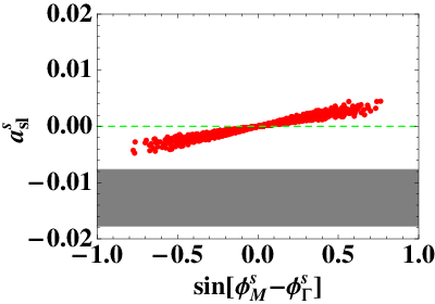
Figure 5: The as​lsa^{s}_{sl}- sin⁡(ϕMs−ϕΓs)\sin{(\phi^{s}_{M}-\phi^{s}_{\Gamma})} (left panel) and as​lsa^{s}_{sl}- mK​Km_{KK} (right panel) correlation plots in the RS model. The gray band indicates the 1σ\sigma experimental allowed ranges for as​lsa^{s}_{sl} (avg). The green line indicates the SM prediction for as​lsa^{s}_{sl}.

We observe that Δ​Ms\Delta M_{s}(exp) constrains |(ULd⁡(1))32||(U^{d(1)}_{L})_{32}| to <∼​10−2\raise 1.29167pt\hbox{$\;<$\kern-7.5pt\raise-4.73611pt\hbox{$\sim\;$}}10^{-2}, and allows rMs,K​K=|M12s,K​K/M12s,S​M|​<∼​1r^{s,KK}_{M}=|M^{s,KK}_{12}/M^{s,SM}_{12}|\raise 1.29167pt\hbox{$\;<$\kern-7.5pt\raise-4.73611pt\hbox{$\sim\;$}}1. Note that similar conclusion about rMs,K​Kr^{s,KK}_{M} was also reached in Ref. [38]. The fit results allow the ratio rΓs,K​K=|Γ12s,K​K/Γ12s,S​M|​<∼​10%r^{s,KK}_{\Gamma}=|\Gamma^{s,KK}_{12}/\Gamma^{s,SM}_{12}|\raise 1.29167pt\hbox{$\;<$\kern-7.5pt\raise-4.73611pt\hbox{$\sim\;$}}10\% for values of mK​K<m_{KK}< 1.5 TeV and this ratio falls quite quickly as mK​Km_{KK} is increased beyond 1.5 TeV. As indicated earlier, NP in b→c​c¯​sb\to c\bar{c}s transitions will also contribute to the lifetimes of bb hadrons. We expect the corrections to the total widths of the bb hadrons to be also <∼​10%\raise 1.29167pt\hbox{$\;<$\kern-7.5pt\raise-4.73611pt\hbox{$\sim\;$}}10\% which cannot be detected experimentally given the hadronic uncertainties in calculating the total widths [48]. The lifetime ratio of the BsB_{s} meson to the BdB_{d} meson, τsS​MτdS​M\frac{\tau_{s}^{SM}}{\tau_{d}^{SM}}, has a tiny theoretical uncertainty in the SM [48]. New physics will contribute equally to the BsB_{s} and BdB_{d} total widths, in the leading order in the heavy quark expansion, thereby largely canceling in the lifetime ratio. Our naive estimate is, NP in b→c​c¯​sb\to c\bar{c}s transition can correct this lifetime ratio as τsτd≈τsS​MτdS​M​(1+x)\frac{\tau_{s}}{\tau_{d}}\approx\frac{\tau_{s}^{SM}}{\tau_{d}^{SM}}(1+x), with x=XΓdS​M​(1−ΓdS​MΓsS​M)x=\frac{X}{\Gamma_{d}^{SM}}\left(1-\frac{\Gamma_{d}^{SM}}{\Gamma_{s}^{SM}}\right) where Γs,dS​M\Gamma_{s,d}^{SM} are the SM Bs,dB_{s,d} widths. Using XΓdS​M​<∼\frac{X}{\Gamma_{d}^{SM}}\raise 1.29167pt\hbox{$\;<$\kern-7.5pt\raise-4.73611pt\hbox{$\sim\;$}} 10 %, τsS​MτdS​M=1±0.01\frac{\tau_{s}^{SM}}{\tau_{d}^{SM}}=1\pm 0.01 [48], we get x​<∼​0.1%x\raise 1.29167pt\hbox{$\;<$\kern-7.5pt\raise-4.73611pt\hbox{$\sim\;$}}0.1\% which is consistent with experimental measurements [16]. In Fig. 5 is shown the as​lsa^{s}_{sl} - sin⁡(ϕMs−ϕΓs)\sin{(\phi^{s}_{M}-\phi^{s}_{\Gamma})} and as​lsa^{s}_{sl}-mK​Km_{KK} correlation plots in the RS model. The gray band indicates the 1σ\sigma experimental allowed ranges for as​lsa^{s}_{sl} (avg) while the green line indicates the SM prediction for as​lsa^{s}_{sl}. As one can see from these figures, the fit results allow as​ls∼−0.00498a^{s}_{sl}\sim-0.00498, which is 1.54​σ1.54\sigma away from its experimental average value in Eq.(12) . The value of the corresponding sin⁡(ϕM−ϕΓs)\sin{(\phi_{M}-\phi^{s}_{\Gamma})} is −0.76-0.76. Hence this model cannot fully account for the experimental results and this is due to the fact that this model cannot generate enough correction to the width difference Δ​Γ12s\Delta\Gamma_{12}^{s}. Note that, as mK​Km_{KK} is increased the suppression to as​lsa^{s}_{sl} due to mK​Km_{KK} is partially compensated by larger mixing angles which are within the considered ranges in this work and are consistent with experimental measurements of Δ​Ms\Delta M_{s} and Δ​Γs\Delta\Gamma_{s}. However, after a certain point the suppression due to mK​Km_{KK} cannot be compensated and as​lsa^{s}_{sl} decreases with increasing mK​Km_{KK} mass.

VI Conclusions

In the past few years several measurements in rare B decays involving b→sb\to s transitions have been somewhat difficult to understand in the SM. This has put the focus on measurements in the Bs0−Bs0¯B_{s}^{0}-{\overline{B_{s}^{0}}} system. The measurements of the phase in Bs0−Bs0¯B_{s}^{0}-{\overline{B_{s}^{0}}} mixing and more recently the like-sign dimuon asymmetry have generated an enormous interest in the community as these measurements indicate possible deviations from the SM predictions. In this work, we presented calculations for general new physics corrections to the parameters in Bs0−Bs0¯B_{s}^{0}-{\overline{B_{s}^{0}}} mixing. Taking the Randall-Sundrum model as an example of new physics we calculated the wrong-charge asymmetry, as​lsa_{sl}^{s}, as well as other parameters in Bs0−Bs0¯B_{s}^{0}-{\overline{B_{s}^{0}}} mixing. Our calculations indicate that while the RS model can cause deviations from the SM predictions for the wrong-charge asymmetry, it cannot explain the present experimental average value within the 1σ\sigma range. This is due its inability to generate sufficient new contribution to the width difference Δ​Γ12s\Delta\Gamma^{s}_{12}, even though the model can generate large contribution to the mass difference Δ​M12s\Delta M^{s}_{12}.

VII Acknowledgements

We would like to thank Q. Shafi, Y. Mimura B. Dutta and Alexander Lenz for useful discussions. The work of S. K. was partially supported by the Science and Technology Development Fund (STDF) Project ID 1855, the ICTP Project ID 30, and the Academy of Scientific Research and Technology. The work of A.D and M.D was supported by the U.S.-Egypt Joint Board on Scientific and Technological Cooperation through the U.S. Department of Agriculture.

References

  • [1] See talk by Kay Kinoshita in DPF 2009.
  • [2] See for example S. Baek, C. W. Chiang and D. London, Phys. Lett. B 675, 59 (2009) [arXiv:0903.3086 [hep-ph]]; S. Baek, P. Hamel, D. London, A. Datta and D. A. Suprun, Phys. Rev. D 71, 057502 (2005) [arXiv:hep-ph/0412086]; M. Duraisamy and A.L. Kagan, Eur. Phys. J. C 70, 921 (2010) [arXiv:0812.3162 [hep-ph]].
  • [3] D. Asner et al. [Heavy Flavor Averaging Group], arXiv:1010.1589 [hep-ex].
  • [4] See for e.g. A. Datta, Phys. Rev. D 66, 071702 (2002) [arXiv:hep-ph/0208016].
  • [5] B. Aubert et al. [BABAR Collaboration], Phys. Rev. Lett. 91, 171802 (2003) [arXiv:hep-ex/0307026]; K. F. Chen et al. [Belle Collaboration], Phys. Rev. Lett. 91, 201801 (2003) [arXiv:hep-ex/0307014].
  • [6] A. Ishikawa et al., Phys. Rev. Lett. 96, 251801 (2006), hep-ex0603018; J. T. Wei et al. [BELLE Collaboration], Phys. Rev. Lett. 103, 171801 (2009) [arXivid0904.0770 [hep-ex]].
  • [7] B. Aubert et al. [BABAR Collaboration], Phys. Rev. D73, 092001 (2006) [hepex0604007], Phys. Rev. D79, 031102 (2009) [arXivid0804.4412 [hep-ex]].
  • [8] “Belle Finds a Hint of New Physics in Extremely Rare B Decays” reported in August 2009 (as Press Release): http://www.kek.jp/intra-e/press/2009/BellePress14e.html.
  • [9] K. Ikado et al., Phys. Rev. Lett. 97, 251802 (2006) [arXiv:hep-ex/0604018].
  • [10] T. Aaltonen et al. [CDF Collaboration], Phys. Rev. Lett. 100, 161802 (2008) [arXiv:0712.2397 [hep-ex]].
  • [11] V. M. Abazov et al. [D0 Collaboration], Phys. Rev. Lett. 101, 241801 (2008) [arXiv:0802.2255 [hep-ex]].
  • [12] See for instance, A. Datta and S. Khalil, Phys. Rev. D 80, 075006 (2009) [arXiv:0905.2105 [hep-ph]]; C. W. Chiang, A. Datta, M. Duraisamy, D. London, M. Nagashima and A. Szynkman, JHEP 1004, 031 (2010) [arXiv:0910.2929 [hep-ph]].
  • [13] A. Lenz et al., arXiv:1008.1593 [hep-ph].
  • [14] V. M. Abazov et al. [DO Collaboration], Phys. Rev. D82 ,032001(2010) [arXiv:1005.2757 [hep-ex]].
  • [15] Y. Grossman, Y.  Nir and G. Raz , Phys. Rev. Lett. 97,151801(2006) [arXiv:hep-ph/0605028].
  • [16] Particle Data Group, C.  Amsler,et al , Phys. Lett. B667, 1(2008), and 2010 edition.
  • [17] V. M. Abazov et al. [DO Collaboration], Phys. Rev. D82 , 012003(2010) [arXiv:0904.3907 [hep-ex]].
  • [18] CDF Collaboration, Note 9015, Oct. 2007.
  • [19] B.  A. Dobrescu, P. J.  Fox and M. Adam  , Phys. Rev. Lett. 105 ,04180(2010) [arXiv:1005.4238 [hep-ph]];
  • [20] A. Dighe, A. Kundu and S. Nandi, arXiv:1005.4051 [hep-ph]; O. Eberhardt, A. Lenz and J. Rohrwild, Phys. Rev. D 82, 095006 (2010) [arXiv:1005.3505 [hep-ph]]; A. Soni, A. K. Alok, A. Giri, R. Mohanta and S. Nandi, Phys. Rev. D 82, 033009 (2010) [arXiv:1002.0595 [hep-ph]]; N. G. Deshpande, X. G. He and G. Valencia, arXiv:1006.1682 [hep-ph]; C. H. Chen and G. Faisel, arXiv:1005.4582 [hep-ph]; C. W. Bauer and N. D. Dunn, arXiv:1006.1629 [hep-ph]; D. Choudhury and D. K. Ghosh, arXiv:1006.2171 [hep-ph]; C. H. Chen, C. Q. Geng and W. Wang, arXiv:1006.5216 [hep-ph]; J. K. Parry, arXiv:1006.5331 [hep-ph]; P. Ko and J. h. Park, arXiv:1006.5821 [hep-ph]; S. F. King, arXiv:1006.5895 [hep-ph]; Y. Bai and A. E. Nelson, arXiv:1007.0596 [hep-ph]; J. Kubo and A. Lenz, arXiv:1007.0680 [hep-ph]; K. Blum, Y. Hochberg and Y. Nir, JHEP 1009, 035 (2010) [arXiv:1007.1872 [hep-ph]]; R. M. Wang, Y. G. Xu, M. L. Liu and B. Z. Li, arXiv:1007.2944 [hep-ph]; B. Dutta, Y. Mimura and Y. Santoso, arXiv:1007.3696 [hep-ph]; A. Lenz et al., arXiv:1008.1593 [hep-ph]; S. Oh and J. Tandean, arXiv:1008.2153 [hep-ph]; S. C. Park, J. Shu, K. Wang and T. T. Yanagida, arXiv:1008.4445 [hep-ph]; W. Chao and Y. c. Zhang, arXiv:1008.5277 [hep-ph]; M. Trott and M. B. Wise, arXiv:1009.2813 [hep-ph]; M. Endo, S. Shirai and T. T. Yanagida, arXiv:1009.3366 [hep-ph]; X. G. He, B. Ren and P. C. Xie, arXiv:1009.3398 [hep-ph]; A. K. Alok, S. Baek and D. London, arXiv:1010.1333 [hep-ph]; The D0 same-charge dimuon asymmetry and possibile new CP violation sources in the Bs−B¯sB_{s}-\bar{B}_{s} system Authors: Jihn E. Kim, Min-Seok Seo, Seodong Shin arXiv:1010.5123v1.
  • [21] C. Delaunay, O. Gedalia, S. J. Lee, G. Perez and E. Ponton, arXiv:1007.0243 [hep-ph].
  • [22] See for example, Z. Ligeti, M. Papucci, G. Perez and J. Zupan, arXiv:1006.0432 [hep-ph].
  • [23] L. Randall and R. Sundrum, Phys. Rev. Lett. 83, 3370 (1999) [arXiv:hep-ph/9905221].
  • [24] T. Gherghetta and A. Pomarol, Nucl. Phys. B 586, 141 (2000) [arXiv:hep-ph/0003129].
  • [25] See for example: S. J. Huber and Q. Shafi, Phys. Lett. B 498, 256 (2001) [arXiv:hep-ph/0010195]. S. J. Huber, Nucl. Phys. B 666, 269 (2003) [arXiv:hep-ph/0303183]. G. Burdman, Phys. Lett. B 590, 86 (2004) [arXiv:hep-ph/0310144]. K. Agashe, G. Perez and A. Soni, Phys. Rev. Lett. 93, 201804 (2004) [arXiv:hep-ph/0406101].
  • [26] K. Agashe, G. Perez and A. Soni, Phys. Rev. D 71, 016002 (2005) [arXiv:hep-ph/0408134].
  • [27] A. Abulencia et al. [CDF Collaboration], Phys. Rev. Lett. 97, 242003 (2006) [arXiv:hep-ex/0609040].
  • [28] V. M. Abazov et al. [D0 Collaboration], Phys. Rev. Lett. 97, 021802 (2006) [arXiv:hep-ex/0603029].
  • [29] A. S. Dighe, I. Dunietz, H. J. Lipkin and J. L. Rosner, Phys. Lett. B 369, 144 (1996) [arXiv:hep-ph/9511363].
  • [30] A. S. Dighe, I. Dunietz and R. Fleischer, Eur. Phys. J. C 6, 647 (1999) [arXiv:hep-ph/9804253].
  • [31] A. Lenz and U. Nierste, JHEP 0706, 072 (2007) [arXiv:hep-ph/0612167]; A. Lenz, Nucl. Phys. Proc. Suppl. 177-178, 81 (2008) [arXiv:0705.3802 [hep-ph]].
  • [32] M. Beneke, G.  Buchalla, C. Greub, A. Lenz and U. Nierste  , Phys. Lett. B459 ,631(1999) [hep-ph/9808385].
  • [33] M. Beneke, G. Buchalla, and I. Dunietz , Phys. Rev. D 54,4419 (1996) arXiv:hep-ph/9605259.
  • [34] A. Dighe, T.  Hurth, C. S. Kim,and T. Yoshikawa , hep-ph/0112067.
  • [35] M. Ciuchini, E. Franco, V. Lubicz, F.Mescia and C. Tarantino , JHEP 08,031. (2003) [arXiv:hep-ph/0308029].
  • [36] A. J. Buras, S. Jager and J. Urban , Nucl. Phys. B 605, 600 (2001) [arXiv:hep-ph/0102316].
  • [37] D. Becirevic, V. Gimenez, G. Martinelli, M. Papinutto and J.  Reyes, JHEP 04, 025 (2002), hep-lat/0110091.
  • [38] M. Blanke, A. J. Buras, B.  Duling, S.  Gori and A. Weiler, JHEP 03, 001 (2009), arXiv:0809.1073[hep-ph].
  • [39] J. Laiho, E. Lunghi and S. R. Van de Water , Rev. Rev. D81,034503(2010) arXiv:0910.2928[hep-ph].
  • [40] A. J. Buras, M. Jamin, and P.  H. Weisz, Nucl. Phys.B347, 491 (1990).
  • [41] A. Agashe, A. Azatov, and L.  Zhu, Phys. Rev.D79, 056006 (2009) arXiv:0810.1016[hep-ph].
  • [42] See S. Khalil and R. Mohapatra, Nucl. Phys. B 695, 313 (2004) [arXiv:hep-ph/0402225]. and references there in.
  • [43] J.  Charles et al [CKMfitter Group], Eur. Phys. J. C41, 1 (2005), hep-ph/0406184.
  • [44] G. Buchalla, A. Buras and M. E. Lautenbacher , Rev. Mod. Phys. 68,1125(1996) arXiv:hep-ph/9512380.
  • [45] C. Csaki, A. Falkowski and A. Weiler, JHEP 0809, 008 (2008) [arXiv:0804.1954 [hep-ph]].
  • [46] O. Gedalia, G. Isidori and G. Perez, Phys. Lett. B 682, 200 (2009) [arXiv:0905.3264 [hep-ph]].
  • [47] K. Agashe, A. Delgado, M. J. May and R. Sundrum, JHEP 0308, 050 (2003) [arXiv:hep-ph/0308036].
  • [48] See A. J. Lenz, AIP Conf. Proc. 1026 (2008) 36 [arXiv:0802.0977 [hep-ph]] and references there in