The leading hadronic vacuum polarisation on the lattice
Abstract
After discussing the relevance of a first principles theory-prediction of the hadronic vacuum polarisation for Standard Model tests, the theoretical challenges for its computation in lattice QCD are reviewed. New ideas that will potentially improve the quality of lattice simulations will be introduced and the status of ongoing simulations will be presented briefly.
Keywords:
chiral Lagrangians, lattice gauge theory, muons, electric momentsClassification:
12.39.Fe; 11.15.Ha; 14.60.Ef; 13.40.Em1 Introduction
The quest to measure the anomalous magnetic moment of the muon, , experimentally with ever increasing precision has started at CERN [1] decades ago and was later continued at BNL [2], yielding a precision of 0.5ppm [3]. In the Standard Model (SM) receives contributions most notably from QED but also from the Weak sector and from QCD. While the former two contributions can be computed in (high order) perturbation theory, the QCD contributions are non-perturbative and as such not computable analytically in a model independent way. As nicely summarised in [4], using unitarity and analyticity, the leading QCD-contribution (cf. figure 1)
is currently determined from the experimental measurement of -annihilation or hadronic -decays. With these experiment-based approaches one is able to predict with a precision below 1%. While the former process seems to provide solid SM-predictions, a pure theory-prediction still seems worth-while. In particular since is sensitive to contributions from physics beyond the SM. In fact, the theory prediction currently differs from the experimental measurement by 3.2 [4]. While not yet providing evidence for new physics, this tension is naturally causing excitement.
2 on the lattice
The leading hadronic contribution is defined as
| (1) |
where the function parametrises the QED contribution to the diagram in figure 1 [9]. Note that the integration is over space-like momenta . The function is the vacuum polarisation amplitude,
where . Simulations of lattice QCD always have to keep track of a number of systematic effects, most notably those stemming from the finite lattice-spacing, the finite volume and unphysically heavy quark masses. These effects have been studied deeply and a large body of tools by now allows one to estimate or to systematically control them at the level of precision required here. In this talk we present new ideas tailored to control systematic uncertainties arising from the presence of quark-disconnected diagrams, from the limited momentum resolution in finite volume field theory and from the contribution of vector resonances.
Quark disconnected diagrams and vector resonances
The electro-magnetic current in eq. (2)
consists of
a linear combination of flavour-diagonal quark-bilinear currents
, where .
The Wick contractions of eq. (2) therefore yield quark connected
contributions
| (3) |
and quark disconnected contributions
| (4) |
where is the quark propagator for the quark flavour and the trace is over spin- and colour-indices. In lattice simulations the latter contribution is often neglected because of the huge overhead its computation causes [10].
A new method for predicting correlation functions consisting of quark-disconnected contributions was developed in [11]. By introducing valence quarks which are degenerate with the dynamical flavours, each Wick contraction can be rewritten in terms of a single fermionic correlation function defined in an unphysical theory. The physical result is recovered by summing over the correlation functions in the unphysical, partially quenched, theory [12, 13, 14]. In particular, the above expectation values eq. (3) and (4) remain unchanged if one of the quarks is replaced by a mass-degenerate partially quenched valence quark . This allows to express them in terms of individual two-point functions, the Wick-contractions of which yield either a connected or a disconnected two-point function:
| (5) | |||
Within partially quenched chiral perturbation theory [12, 13, 14, 15, 16], expressions for the connected and the disconnected contributions to hadronic correlation functions can be computed. The case of the -theory without and with a partially quenched strange quark as well as the -theory were studied in [11]. In the -theory for example, the calculation at next-to-leading order in the effective theory predicts that the disconnected contribution reduces the connected contribution by only 10%.
The analytical prediction of quark-disconnected diagrams is work in progress. In particular, vector resonances which are not dynamical degrees of freedom in chiral perturbation theory turn out to be dominating [6, 7]. It will be interesting to study the impact of vector resonances on the above predictions by including these degrees of freedom into the chiral Lagrangian [17]. However, while the effective theory for pions and kaons stands on solid grounds, this similar ansatz for vector mesons is a model.
Momentum resolution
Today, typical lattices extend over fm in the spatial directions
(typically twice that large in the temporal direction, ).
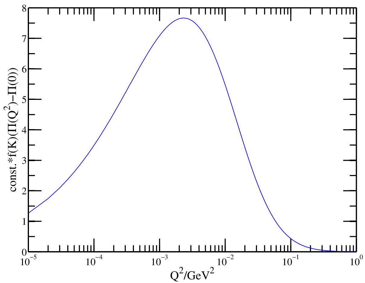
Besides vanishing momentum, the lowest hadron momentum therefore corresponds to the lowest non-vanishing Fourier-mode, MeV. The plot in figure 2 shows the integral kernel of eq. (1), which is peaked at around the muon mass, MeV. The lattice data therefore needs to be extrapolated into this region. In order to compute closer to the peak, the Mainz group [8] is applying twisted boundary conditions to the valence quark fields, , which allows one to tune the offset of the Fourier Modes accessible in the lattice computation [18, 19, 20, 21, 22, 23, 24]. Naively, the twists applied to the quark-fields in the flavour-diagonal currents in eq. (2) will cancel (see e.g. [20]). However, the connected correlation function in eq. (5), , is composed of flavour-off-diagonal currents. Hence, different twist-angles can be applied for the quark fields and , respectively [11]. This argument allows to apply partial twisting at least to the connected contribution to . The disconnected contribution can either be predicted using chiral perturbation theory (cf. above) or it can be computed for the usual Fourier momenta and then be interpolated using the ansatz provided by chiral perturbation theory. Figure 3 shows results for by the Mainz group.

Without twisting only the blue data points are accessible, while with
twisting the red
data points can be added. Besides providing data points closer to the region
where the integral eq. (1) receives major contributions, the
additional data points for larger values of the momentum will help in stabilising fits:
In order to compute the result for the vacuum polarisation tensor eq. (2)
one first fits an ansatz for its momentum-dependence to the data and then
integrates it. The Mainz group uses
models for the vector resonance, polynomials and Padé approximations
as ansätze (cf. also ETM’s study of parametrisations of vector resonances
in [7]). An estimate of the systematic
uncertainties is obtained from the spread of the respective fit-results.
In our analysis the additional data points which we obtained by using
partially twisted boundary conditions helped to reduce this spread significantly.
3 Status
Figure 4 shows results for the vacuum polarisation by
ETM [7], MILC [6]
and by the Mainz group. Note that Mainz is the only group using
twisted boundary conditions while ETM is the only collaboration trying
to compute the disconnected contribution directly. For comparison we
quote the value obtained from the analysis of -annihilation,
[4]. Clearly the lattice
data tend towards
this value as the quark mass is reduced, but the extrapolation to the physical
point is model-dependent and will only be dispensable once the simulation is
carried out for physical quark masses.

In this talk we present the status of lattice computations of
. While significant progress has been made recently systematic
uncertainties are still not under sufficient control. Clearly, simulations
at the physical point would be very desirable in order to be independent of
model-based extrapolations of lattice data.
References
- (1) G. Charpak, et al., Phys. Rev. Lett. 6, 128–132 (1961).
- (2) G. W. Bennett, et al., Phys. Rev. Lett. 92, 161802 (2004).
- (3) G. Bennett, et al., Phys.Rev. D73, 072003 (2006).
- (4) F. Jegerlehner, and A. Nyffeler, Phys.Rept. 477, 1–110 (2009).
- (5) M. Gockeler, et al., Nucl.Phys. B688, 135–164 (2004).
- (6) C. Aubin, and T. Blum, Phys.Rev. D75, 114502 (2007).
- (7) D. B. Renner, X. Feng, K. Jansen, and M. Petschlies (2010).
- (8) B. Brandt, S. Capitani, M. Della Morte, D. Djukanovic, G. von Hippel, et al. (2010).
- (9) B. e. Lautrup, A. Peterman, and E. de Rafael, Phys. Rept. 3, 193–260 (1972).
- (10) H. Neff, N. Eicker, T. Lippert, J. W. Negele, and K. Schilling, Phys.Rev. D64, 114509 (2001).
- (11) M. Della Morte, and A. Juttner (2010).
- (12) C. W. Bernard, and M. F. L. Golterman, Phys. Rev. D46, 853–857 (1992).
- (13) C. W. Bernard, and M. F. Golterman, Phys.Rev. D49, 486–494 (1994).
- (14) S. R. Sharpe, and N. Shoresh, Phys. Rev. D62, 094503 (2000).
- (15) J. Gasser, and H. Leutwyler, Ann. Phys. 158, 142 (1984).
- (16) J. Gasser, and H. Leutwyler, Nucl. Phys. B250, 465 (1985).
- (17) G. Ecker, J. Gasser, A. Pich, and E. de Rafael, Nucl.Phys. B321, 311 (1989).
- (18) P. F. Bedaque, Phys. Lett. B593, 82–88 (2004).
- (19) G. M. de Divitiis, R. Petronzio, and N. Tantalo, Phys. Lett. B595, 408–413 (2004).
- (20) C. T. Sachrajda, and G. Villadoro, Phys. Lett. B609, 73–85 (2005).
- (21) P. F. Bedaque, and J.-W. Chen, Phys. Lett. B616, 208–214 (2005).
- (22) B. C. Tiburzi, Phys. Lett. B617, 40–48 (2005).
- (23) J. M. Flynn, A. Jüttner, and C. T. Sachrajda, Phys. Lett. B632, 313–318 (2006).
- (24) D. Guadagnoli, F. Mescia, and S. Simula, Phys. Rev. D73, 114504 (2006).