Secure Index Coding with Side Information
Abstract
Security aspects of the Index Coding with Side Information (ICSI) problem are investigated. Building on the results of Bar-Yossef et al. (2006), the properties of linear coding schemes for the ICSI problem are further explored. The notion of weak security, considered by Bhattad and Narayanan (2005) in the context of network coding, is generalized to block security. It is shown that the coding scheme for the ICSI problem based on a linear code of length , minimum distance and dual distance , is -block secure (and hence also weakly secure) if the adversary knows in advance messages, and is completely insecure if the adversary knows in advance more than messages.
I Introduction
The problem of Index Coding with Side Information (ICSI) was introduced by Birk and Kol [1], [2]. It was motivated by applications such as audio and video-on-demand, and daily newspaper delivery. In these applications a server (sender) has to deliver some sets of data, audio or video files to the set of clients (receivers), different sets are requested by different receivers. Assume that before the transmission starts, the receivers have already (from previous transmissions) some files or movies in their possession. Via a slow backward channel, the receivers can let the sender know which messages they already have in their possession, and which messages they request. By exploiting this information, the amount of the overall transmissions can be reduced. As it was observed in [1], this can be achieved by coding the messages at the server before broadcasting them out.
Another possible application of the ICSI problem is in opportunistic wireless networks. These are the networks in which a wireless node can opportunistically listen to the wireless channel. As a result, the node may obtain packets that were not designated to it (see [3, 4, 5]). This way, a node obtains some side information about the transmitted data. Exploiting this additional knowledge may help to increase the throughput of the system.
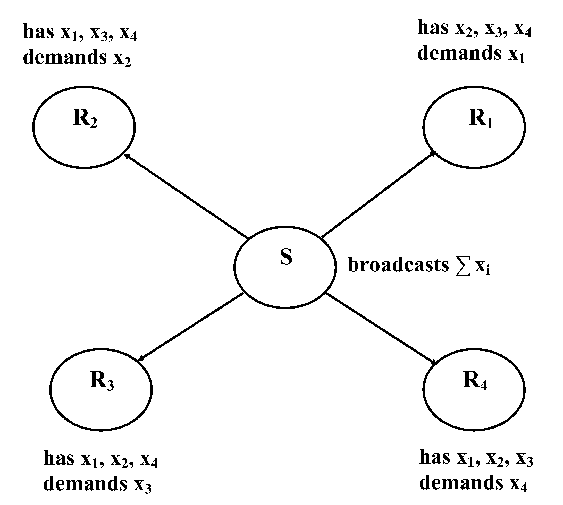
Consider the toy example in Figure 1. It presents a scenario with one sender and four receivers. Each receiver requires a different information packet (or message). The naïve approach requires four separate transmissions, one transmission per an information packet. However, by exploiting the knowledge about the subsets of messages that clients already have, and by using coding of the transmitted data, the server can satisfy all the demands by broadcasting just one coded packet.
The ICSI problem has been a subject of several recent studies [6, 7, 8, 9, 10, 3, 11, 12]. This problem can be regarded as a special case of the well-known network coding (NC) problem [13]. In particular, it was shown that every instance of the NC problem can be reduced to an instance of the ICSI problem [10, 3].
Several previous works focused on the design of an efficient scheme for the ICSI problem. Bar-Yossef et al. [6] proved that finding the best scalar linear binary solution for the ICSI problem is equivalent to finding the so-called minrank of a graph, which is known to be an NP-hard problem (see [6, 14]). Here scalar linear solutions refer to linear schemes in which each message is a symbol in the field . By contrast, in vector linear solutions each message is a vector over . Lubetzky and Stav [7] showed that there exist instances in which scalar linear solutions over nonbinary fields and linear solutions over mixed fields outperform the scalar linear binary solutions. The latter were also studied by Bar-Yossef et al. [6].
El Rouayheb et. al.[10, 3] and Alon et al. [12] showed that for certain instances of the ICSI problem, vector linear solutions achieve strictly higher transmission rate than scalar linear solutions do. They also pointed out that there exist instances in which nonlinear codes outperform linear codes. Several heuristic solutions for the ICSI problem were proposed in [9, 11].
In this paper, we study the security aspect of a linear solution for the ICSI problem. We show that every linear scheme provides a certain level of security. More specifically, let and be the length and the dimension of the code , associated with a particular ICSI instance. Let and be its minimum distance and dual distance, respectively. We say that a particular adversary is of strength if it has packets of information in its possession. Then, we show that a scheme employing the code is -block secure against all adversaries of strength and is completely insecure against any adversary of strength at least . If the code is MDS, then the two bounds coincide.
The paper is organized as follows. Notations and definitions, which are used in the rest of the paper, are introduced in Section II. The model and some basic results for the ICSI problem are presented in Section III. The security properties of linear ICSI schemes are analyzed in Section IV. The main results of this paper appear in that section. Finally, the paper is concluded in Section V.
II Preliminaries
We use the notation for the finite field of elements, where is a power of prime, and for the set of all nonzero elements of . We also use to denote the set of integers . For the vectors and , the (Hamming) distance between and is defined to be the number of coordinates where and differ, namely,
The support of a vector is defined to be the set . The (Hamming) weight of a vector , denoted , is defined to be , the number of nonzero coordinates of .
A -dimensional subspace of is called a linear (-ary) code if the minimum distance of ,
is equal to . Sometimes we may use the notation for the sake of simplicity. The vectors in are called codewords. It is easy to see that the minimum weight of a nonzero codeword in a linear code is equal to its minimum distance . A generator matrix of an -code is a matrix whose rows are linearly independent codewords of . Then .
The dot product of the two vectors is defined to be . Thus, , the normal matrix product of and , where denotes the transpose of . The dual code or dual space of is defined as . The minimum distance of , , is called the dual distance of .
The following upper bound on the minimum distance of a -ary linear code is well-known (see [15] Chapter 1).
Theorem II.1 (Singleton bound)
For an -code, we have .
Codes attaining this bound are called maximum distance separable (MDS) codes. For a subset of vectors
define its linear span:
We use to denote the unit vector, which has a one at the th position, and zeros elsewhere. We also use , , to denote the identity matrix.
We recall the following well-known result in coding theory.
Theorem II.2 ([16], p. 66)
Let be an -code with dual distance and denote the matrix whose rows are codewords of . If then each -tuple from appears in an arbitrary set of columns of exactly times.
For a random vector and a subset of , where , let denote the vector . For a matrix , let denote the th column of , and its th row. For a set , let denote the matrix obtained from by deleting all the columns of which are not indexed by the elements of .
Let and be discrete random variables taking values in the sets and , respectively. Let denote the probability that takes a particular value . The (binary) entropy of is defined as
The conditional entropy of given is defined as
This definition can be naturally extended to
for discrete random variables , .
If the probability distribution of is unchanged given the knowledge of , i.e., for all , , then . Indeed, equals
III Index Coding and Some Basic Results
III-A Linear Coding Model
Index coding problem considers the following communications scenario. There is a unique sender (or source) , who has a vector of messages in his possession, which is a realized value of a random vector . hereafter are assumed to be independent uniformly distributed random variables over . There are also receivers . For each , has some side information, i.e. owns a subset of messages , . In addition, each , , is interested in receiving the message , for some demand function . Hereafter, we assume that every receiver requests exactly one message. The scenario, where each receiver requests more than one message, is discussed in Section III-B.
Let and . In the sequel, we write if for any it holds . Intuitively, this means that if some receiver knows for all (and also knows ), then this receiver is also able to compute the value of .
In this paper we consider linear index coding. In particular, we assume that broadcasts a vector of linear combinations , each combination is of the form
for , where is a linearly independent set of vectors in . Let the code of length and dimension over be defined as
Hereafter, we assume that the sets for are known to . Moreover, we also assume that the code is known to each receiver , . In practice this can be achieved by a preliminary communication session, when the knowledge of the sets for and of the code are disseminated between the participants of the scheme.
The following lemma was formulated in [6] for the case where is a binary field. This lemma specifies a sufficient condition on so that the coding scheme is successful, i.e. any has enough data to reconstruct , , at the end of the communication session. We reproduce this lemma (for the general ) with its proof for the sake of completeness of the presentation.
Lemma III.1
Let be an -code and let be a basis of . Suppose broadcasts vector . Then, for each , the receiver can reconstruct if the following two conditions hold:
- 1.
there exists such that ;
- 2.
the vector is in .
Proof:
Assume that and . Since , we obtain that there exist such that
By multiplying by , we obtain that
| (1) | |||||
Therefore,
Observe that is able to find and all from the knowledge of the code . Moreover, is also able to compute since . Therefore, is able to compute . ∎
Lemma III.1 suggests that in order for the receivers to recover their desired symbols, can use the code , for some , . We show later in Corollary IV.3 that must use a code of such form to guarantee a successful communication session. Finding the lowest dimension code by careful selection of ’s is a difficult task (in fact it is NP-hard to do so, see [6, 14]), which, however, yields a scheme with the minimal number of transmissions.
III-B Receivers with Multiple Requests
Consider a more general ICSI problem where each receiver requests more than one message. This problem was discussed in [1]. It was shown therein that there exists an equivalent problem with one requested message per each receiver. This new problem is easily obtained by splitting each receiver, which requests messages, into different receivers with the same side information, where each receiver requests exactly one message. For more detail, the reader can refer to [1]. In the sequel, we consider scenarios, where each receiver requests exactly one message.
III-C Scalar and Vector Solutions
The type of linear solutions considered in this model are referred to as scalar linear solutions in [10, 12]. For vector linear solutions, each message is divided into several packets, each packet is a symbol in , and a coding scheme combines packets from different messages to minimize the number of transmissions. It was shown in [12] (see also [3], [10]) that there exist instances of the problem in which a vector linear solution has significantly higher transmission rate than any scalar linear solution. Here, the transmission rate of a scheme is defined as the number of packet transmissions required for delivery of one packet to each receiver.
However, if each message consists of packets (symbols in ), then a vector linear solution of this instance can be regarded as a scalar linear solution (over ) of another instance of the index coding problem, where each receiver requests exactly messages in . This instance, in turn, is equivalent to an instance of the ICSI problem considered in this paper. Therefore, the two identical -ary linear codes of length can be used for these two equivalent ICSI problems. In that case, in order to study the security of the vector linear solution of an instance of the ICSI problem, it is enough to study the security of the equivalent scalar linear solution of some other instance of the ICSI problem.
IV Block Secure Linear Index Coding
IV-A Block Security and Weak Security
In Section IV, we present our main results. Hereafter, we assume the presence of an adversary who can listen to all transmissions. Let be an -code, and be a basis of . Let be a generator matrix of whose rows are . Suppose broadcasts . The adversary is assumed to possess side information , where . For short, we say that knows . The strength of an adversary is defined to be . Denote . Note that from listening to , the adversary also knows . We define below several levels of security for ICSI schemes.
Definition IV.1
Consider an ICSI scheme, which is based on a linear code . The sender possesses a vector of messages , which is a realized value of a random vector . An adversary possesses .
- 1.
For , the adversary is said to have no information about if
(2) In other words, despite the partial knowledge on that the adversary has (his side information and the symbols he overheard), the symbols still looks completely random to him.
- 2.
The scheme is said to be -block secure against if for every -subset , the adversary has no information about .
- 3.
The scheme is said to be -block secure against all adversaries of strength () if it is -block secure against for every , .
- 4.
The scheme is said to be weakly secure against if it is -block secure against . In other words, after listening to all transmissions, the adversary has no information about each particular message that he does not possess in the first place.
- 5.
The scheme is said to be weakly secure against all adversaries of strength () if it is weakly secure against for every -subset of .
- 6.
The scheme is said to be completely insecure against if an adversary, who possesses , by listening to all transmissions, is able to determine for all .
- 7.
The scheme is said to be completely insecure against any adversary of strength () if an adversary, who possesses an arbitrary set of messages, is always able to reconstruct all of the other messages after listening to all transmissions.
Even when the scheme is -block secure () as defined above, the adversary is still able to obtain information about dependencies between various ’s in (but he gains no information about any group of particular messages). This definition of -block security is a generalization of that of weak security (see [17], [18]). Obviously, if a scheme is -block secure against () then it is also weakly secure against , but the converse is not always true.
IV-B Necessary and Sufficient Conditions for Block Security
In the sequel, we consider the sets , , and , . Moreover, we assume that the sets , , and are disjoint, and that they form a partition of , namely . In particular, .
Lemma IV.1
Assume that for all and for all , (not all ’s are zeros),
| (3) |
Then,
- 1.
for all :
(4) - 2.
the system
(5) has at least one solution for every choice of .
Proof:
- 1.
If then the first claim follows immediately. Otherwise, assume that . As the rows of are linearly dependent, there exists such that .
- •
If for all such and for all we have , then for all .
- •
Otherwise, there exist and such that and . Without loss of generality, assume that . Let . Then
Hence and . Let and for all . Then ’s are not all zero and , which contradicts (3).
- •
- 2.
∎
The following lemma provides us with a criteria to decide whether a particular scheme (based on a code ) is block secure against the adversary or not. This lemma is a generalization of Lemma III.1 in the following senses. First, while Lemma III.1 does not discuss security, observe that the adversary can be viewed as one of the receivers. Then, the sufficient conditions (1) and (2) in Lemma III.1 (when applied to and ) are also sufficient conditions for successful reconstruction of a symbol by . Below, we show that these conditions are also necessary. Additionally, in the lemma below, the weak security, implied by the aforementioned generalization, is further extended to block security. (Note that similar statement can be formulated with respect to receivers .)
Lemma IV.2
For a subset , the adversary, after listening to all transmissions, has no information about if and only if
| (6) |
In particular, for each , has no information about if and only if
Proof:
Assume that (6) holds. We need to show that the entropy of is not changed given the knowledge of and . Hence, as shown in Section II, it suffices to show that for all :
| (7) |
Consider the following linear system with the unknown
which is equivalent to
| (8) |
In order to prove that (7) holds, it suffices to show that for all choices of , (8) always has the same number of solutions . Notice that the number of solutions of (8) is equal to the number of solutions of
| (9) |
where , , and are known. For any , if (9) has a solution, then it has exactly different solutions. Therefore, it suffices to prove that (9) has at least one solution for every .
Since is an obvious solution of (8), we have
| (10) |
Subtract (10) from (9) we obtain
which can be rewritten as
| (11) |
where , . Due to Lemma IV.1, (11) always has a solution , for every choice of . Therefore (9) has at least one solution for every .
Now we prove the converse. Assume that (6) does not hold. Then there exists and , , where ’s, are not all zero, such that
for some . Hence, similar to the proof of Lemma III.1, the adversary obtains
Note that the adversary can calculate from , and can also find based on his own side information. Therefore, is able to compute a nontrivial linear combination of ’s, . Hence the entropy . Thus, the adversary has some information about the . ∎
We have the following straight-forward corollary. It generalizes Lemma III.1 by providing both the necessary and sufficient conditions for the weak security. (Note, that this corollary considers the receiver rather than the adversary , since the arguments of Lemma IV.2 also apply to all receivers.)
Corollary IV.3
For each , the receiver can reconstruct , , if and only if
- 1.
there exists such that ;
- 2.
the vector is in .
Corollary IV.3 suggests that in order for the receivers to recover their desired messages, it is necessary and sufficient to employ a code of the form , for some , .
Theorem IV.4
Suppose that the source broadcasts
where is a basis of , for some , . Let be the minimum distance of . Then
- 1.
The scheme is -block secure against all adversaries of strength . In particular, the scheme is weakly secure against all adversaries of strength .
- 2.
The scheme is not weakly secure against at least one adversary of strength . More generally, if there exists a codeword of weight , then the scheme is not weakly secure against at least one adversary of strength .
- 3.
Every adversary of strength is able to determine a list of vectors in which includes the vector of messages .
Proof:
- 1.
- 2.
We now show that the scheme is not weakly secure against at least one adversary of strength . The more general statement can be proved in an analogous way.
Pick a codeword such that and let . Take , . Let
Then, and . By Lemma III.1, is able to determine . Hence the scheme is not weakly secure against the adversary , who knows messages ’s in advance.
- 3.
Consider the following linear system of equations with unknown
which is equivalent to
(13) The adversary attempts to solve this system. Given that and are known, the system (13) has unknowns and equations. Note that , and thus by Theorem II.1 we have . If then (13) has exactly solutions, as required.
Next, we show that . Assume, by contrary, that the rows of , denoted by , are linearly dependent. Then there exist , , not all zero, such that . Let
(Recall that denotes the -th row of ). Then and hence . This is a contradiction, which follows from the assumption that the rows of are linearly dependent.
∎
Example IV.1
Let . Assume that and that for all . Consider a linear scheme for the ICSI problem, employing an -code with , which is defined as follows. For each choose some . Let . Then, indeed, . Since , we have . Therefore by Theorem IV.4 the scheme employing is weakly secure against . Moreover, if is nontrivial (and so ), we have .
IV-C Block Security and Complete Insecurity
Theorem IV.4 provides a threshold for the security level of a scheme that uses a given linear code . If has a prior knowledge of any messages, then the scheme is still secure, i.e. the adversary has no information about any particular messages from . On the other hand, the scheme may no longer be secure against an adversary of strength . The last assertion of Theorem IV.4 shows us the difference between being block secure and being (strongly) secure in a commonly used sense (see, for instance [19]). More specifically, if the scheme is (strongly) secure, the messages look completely random to the adversary, i.e. the probability to guess the correct messages is . However, if the scheme is -block secure (for ), then the adversary is able to guess the correct messages with probability .
For an adversary of strength , the security of the scheme depends on the properties of the code employed, in particular, it depends on the weight distribution of . From Theorem IV.4, if there exists with , then the scheme is not weakly secure against some adversary of strength . In general, the scheme might still be (-block or weakly) secure against some adversaries of strength for . While we cannot make a general conclusion on the security of the scheme when the adversary’s strength is larger than , Lemma IV.2 is still a useful tool to evaluate the security in that situation. However, as the next theorem shows, if the size of is sufficiently large, then is able to determine all the messages in .
Theorem IV.5
Suppose that the settings of the coding scheme for the ICSI problem are defined as in Theorem IV.4. Then the scheme is completely insecure against any adversary of strength , where denotes the dual distance of .
Proof:
Suppose the adversary knows a subset , and . By Corollary IV.3, it suffices to show that for all , there exists satisfying simultaneously and .
Indeed, take any , and let . Consider the indices which are not in . By Theorem II.2, there exists a codeword with
Then . We define such that , as follows. For , we set , and for , we set . It is immediately clear that . Therefore, by Corollary IV.3, the adversary can reconstruct . We have shown that the scheme is completely insecure against an arbitrary set satisfying , hence completing the proof. ∎
When is an MDS code, we have , and hence the two bounds established in Theorems IV.4 and IV.5 are actually tight. The following example further illustrates the results stated in these theorems.
Example IV.2
Let . Suppose that the receivers have in their possession set of messages as appears in the third column of the table below. Suppose also, that the demands of all receivers are as in the second column of the table.
For , let such that . Assume that this scheme uses the code . Then the set forms a basis for . It is easy to see that this is a Hamming code with and .
Suppose that broadcasts the following four bits:
,
,
,
.
Each , , can compute by using linear combination of . Then, each can subtract (his side information) from to retrieve .
For example, consider . Since
subtracts from to obtain
If an adversary has a knowledge of a single message , then by Theorem IV.4, is not able to determine any other message , for . Indeed, , while . Therefore, the scheme is weakly secure against all adversaries of strength . Similarly, if the adversary knows none of the messages in advance, then the adversary has no information about any group of messages. On the other hand, the scheme is completely insecure against any adversary of strength ; in that case is able to recover the remaining messages.
IV-D Role of the Field Size
The following example demonstrates that the use of codes over larger fields might have a positive impact on the security level. More specifically, in that example, codes over large fields significantly enhance the security, compared with the codes over small field.
Example IV.3
Suppose that the source has messages . Assume that there are receivers , and each receiver has the same set of side information, . Assume also that each requires , for .
We can define the ICSI scheme based on the code , as above. The code employed in this scheme has dimension at least , since all the vectors , for some , , are linearly independent. Therefore, the number of transmission required in this scheme is at least , which is equal to the number of transmissions in the trivial solution (just broadcasting each of ).
If we employ a binary code , for the large values of the minimum distance of is bounded from above by a sphere-packing bound
where as . Hence the scheme, which uses a binary code, is secure against any adversary of strength . It is insecure against some adversaries of strength .
There is a variety of stronger upper bounds on the minimum distance of binary codes, such as the Johnson bound, the Elias bound, and the McEliece-Rodemich-Rumsey-Welch bound (see [20, Chapter 4.5] for more details). These bounds provide even stronger bounds on the security of this ICSI scheme, when the scheme is based on the binary code.
By contrast, consider an -ary code , for (we also assume here that all are in ). There exists a -ary MDS code of length , dimension , and with the minimum distance equal (for example, Reed-Solomon code). By employing this code, the new scheme is secure against all adversaries of strength . In order to find an appropriate generator matrix for the Reed-Solomon code for the settings of this example, we start with some generator matrix of Reed-Solomon code, and then apply Gaussian elimination to obtain a new generator matrix of the form , where is a matrix over .
It is well known that there is a significant gap between the Singleton bound and the sphere-packing bound (see [20, p. 111] for details). Therefore, for some ICSI instances, coding over large fields can provide significantly higher levels of security than binary coding.
V Conclusion and Open Questions
In this paper, we analyze the levels of security of linear solutions for the ICSI problem and establish two new bounds. These bounds employ the minimum distance and the dual distance of the linear code used in the scheme. While the dimension of this code corresponds to the number of transmissions in the scheme, the minimum distance is related to the security of the scheme. The generating matrix of the code depends on the sets of messages that each receiver owns.
However, there are various generating matrices that can be used for the same instance of ICSI problems. Moreover, puncturing of some nonzero entries in the generating matrix, could probably lead to a code with a better minimum distance, which in turn corresponds to a ICSI scheme with stronger security. Thus, the question which remains open is how to design a code for a particular instance of the ICSI problem, which has the largest possible minimum distance. It is very likely that finding such a code is a hard problem. For comparison, even finding the minimum distance of a code given by its generating matrix is known to be NP-hard [21].
The following simple generalization of the ICSI problem is called Network Coding with Side Information (NCSI) problem. Consider a network with a sender , possessing messages, and receivers . Each requests one message. Suppose that each has some side information, namely knows some subset of these messages. There is also an adversary , listening to some links in the network, who possesses some of the messages. Given an instance of the NCSI problem, the following questions arise:
- 1.
Is it possible to satisfy all the requests simultaneously by a single transmission, using linear network coding?
- 2.
If there exists network coding solution, how secure is it?
Some techniques, presented in this paper, can be extended to provide sufficient (and sometimes necessary) conditions for an existence of a linear solution for the NCSI problem, and to analyze the level of security of such a solution. We omit the details from this paper.
VI Acknowledgements
The authors would like to thank Frédérique Oggier for helpful discussions. This work is supported by the National Research Foundation of Singapore (Research Grant NRF-CRP2-2007-03).
References
- [1] Y. Birk and T. Kol, “Informed-source coding-on-demand (ISCOD) over broadcast channels,” in Proc. IEEE Conf. on Comput. Commun. (INFOCOM), San Francisco, CA, 1998, pp. 1257–1264.
- [2] ——, “Coding-on-demand by an informed source (ISCOD) for efficient broadcast of different supplemental data to caching clients,” IEEE Trans. Inform. Theory, vol. 52, no. 6, pp. 2825–2830, 2006.
- [3] S. El Rouayheb, A. Sprintson, and C. Georghiades, “On the index coding problem and its relation to network coding and matroid theory,” submitted to IEEE Trans. Inform. Theory.
- [4] S. Katti, H. Rahul, W. Hu, D. Katabi, M. Médard, and J. Crowcroft, “Xors in the air: Practical wireless network coding,” in Proc. ACM SIGCOMM, 2006, pp. 243–254.
- [5] S. Katti, D. Katabi, H. Balakrishnan, and M. Médard, “Symbol-level network coding for wireless mesh networks,” ACM SIGCOMM Comput. Commun. Review, vol. 38, no. 4, pp. 401–412, 2008.
- [6] Z. Bar-Yossef, Z. Birk, T. S. Jayram, and T. Kol, “Index coding with side information,” in Proc. 47th Annu. IEEE Symp. on Found. of Comput. Sci. (FOCS), 2006, pp. 197–206.
- [7] E. Lubetzky and U. Stav, “Non-linear index coding outperforming the linear optimum,” Proc. 48th Annu. IEEE Symp. on Found. of Comput. Sci. (FOCS), pp. 161–168, 2007.
- [8] Y. Wu, J. Padhye, R. Chandra, V. Padmanabhan, and P. A. Chou, “The local mixing problem,” in Proc. Inform. Theory and Applicat. Workshop, San Diego, CA, 2006.
- [9] S. El Rouayheb, M. A. R. Chaudhry, and A. Sprintson, “On the minimum number of transmissions in single-hop wireless coding networks,” in Proc. IEEE Inform. Theory Workshop (ITW), 2007, pp. 120–125.
- [10] S. El Rouayheb, A. Sprintson, and C. Georghiades, “On the relation between the index coding and the network coding problems,” in Proc. IEEE Symp. on Inform. Theory (ISIT), Toronto, Canada, 2008, pp. 1823–1827.
- [11] M. A. R. Chaudhry and A. Sprintson, “Efficient algorithms for index coding,” in Proc. IEEE Conf. on Comput. Commun. (INFOCOM), 2008, pp. 1–4.
- [12] N. Alon, A. Hassidim, E. Lubetzky, U. Stav, and A. Weinstein, “Broadcasting with side information,” in Proc. 49th Annu. IEEE Symp. on Found. of Comput. Sci. (FOCS), 2008, pp. 823–832.
- [13] R. Ahlswede, N. Cai, S. Y. R. Li, and R. W. Yeung, “Network information flow,” IEEE Trans. Inform. Theory, vol. 46, pp. 1204–1216, 2000.
- [14] R. Peeters, “Orthogonal representations over finite fields and the chromatic number of graphs,” Combinatorica, vol. 16, no. 3, pp. 417–431, 1996.
- [15] F. J. MacWilliams and N. J. A. Sloane, The Theory of Error-Correcting Codes. Amsterdam: North-Holland, 1977.
- [16] A. S. Hedayat, N. J. A. Sloane, and J. Stufken, Orthogonal Arrays: Theory and Applications. New York: Springer-Verlag, 1999.
- [17] K. Bhattad and K. R. Narayanan, “Weakly secure network coding,” in Proc. 1st Workshop on Network Coding, Theory, and Applicat. (NetCod), 2005.
- [18] D. Silva and F. R. Kschischang, “Universal weakly secure network coding,” in Proc. Inform. Theory Workshop on Networking and Inform. Theory (ITW), 2009, pp. 281–285.
- [19] N. Cai and R. W. Yeung, “Secure network coding,” in Proc. IEEE Int. Symp. Inform. Theory (ISIT), Lausanne, Switzerland, 2002.
- [20] R. Roth, Introduction to Coding Theory. Cambridge, United Kingdom: Cambridge University Press, 2006.
- [21] A. Vardy, “The intractability of computing the minimum distance of a code,” IEEE Trans. Inform. Theory, vol. 43, no. 6, pp. 1757–1766, 1997.