Light Stop Searches at the LHC in Events with two b–Jets and Missing Energy

Preprint: DO-TH 10/17Preprint: SCIPP 10/19Preprint: BONN-TH-2010-08

S. Bornhauser Email: bornhaus@th.physik.uni-bonn.de Affiliation: Department of Physics and Astronomy, University of New Mexico, Albuquerque, NM 87131, USA M. Drees Email: drees@th.physik.uni-bonn.de Affiliation: BCTP and Physics Institute, University of Bonn, Bonn, Germany and
School of Physics, KIAS, Seoul 130–722, Korea S. Grab Email: sgrab@scipp.ucsc.edu Affiliation: Santa Cruz Institute for Particle Physics, University of California, Santa Cruz, California 95064, USA J.S. Kim Email: jongsoo.kim@tu-dortmund.de Affiliation: Institut für Physik, Technische Universität Dortmund, D-44221 Dortmund, Germany

Abstract

We propose a new method to discover light top squarks (stops) in the co–annihilation region at the Large Hadron Collider (LHC). The bino–like neutralino is the lightest supersymmetric particle (LSP) and the lighter stop is the next–to–LSP. Such scenarios can be consistent with electroweak baryogenesis and also with dark matter constraints. We consider the production of two stops in association with two $b-$ quarks, including pure QCD as well as mixed electroweak–QCD contributions. The stops decay into a charm quark and the LSP. For a higgsino–like light chargino the electroweak contributions can exceed the pure QCD prediction. We show the size of the electroweak contributions as a function of the stop mass and present the LHC discovery reach in the stop–neutralino mass plane.

I Introduction

The Large Hadron Collider (LHC) is currently collecting data at $\sqrt{s}=7\,\mathrm{TeV}$ and it is assumed that the integrated luminosity will reach $1\,\mathrm{fb^{-1}}$ next year. If low–energy supersymmetry (SUSY) [1] is realized, detection of light supersymmetric particles may be around the corner [2].

The scalar top (stop) within the minimal supersymmetric standard model (MSSM) [1] is naturally one of the lightest SUSY particles (sparticles). On the one hand, the large top Yukawa coupling leads to large mixing between left– and right–handed stops, reducing the mass of the lightest stop mass eigenstate. On the other hand, the large top Yukawa coupling reduces the stop mass at the electroweak (EW) scale via renormalization group equation (RGE) running [3]. The lightest stop, $\tilde{t}_{1}$ , is mostly right–handed, since $m_{\tilde{t}_{R}}$ is not increased by $SU(2)$ gaugino loops, and is more strongly reduced by the top Yukawa interaction [3].

A light stop with a mass of $m_{\tilde{t}_{1}}\lesssim 125$ GeV is vital for successful EW baryogenesis within the MSSM [4, 5, 6, 7, 8, 9]. It allows for a strong first order phase transition, which prevents the generated baryon asymmetry of the universe [10, 11] from being washed out. Furthermore, CP violation is needed in order to generate the baryon asymmetry [12]. The Standard Model (SM) CP violating Dirac phase is too small [13], whereas the MSSM contains additional CP–violating phases sufficient for EW baryogenesis [7].

However, new CP violating phases are strongly constrained by the non–observation of electric dipole moments ruling out large regions of the MSSM consistent with EW baryogenesis [14, 6, 9, 8]. Of the remaining MSSM parameter space, scenarios with bino–driven baryogenesis are probably the most promising ones [6, 9]. Here, CP violation in the bino–higgsino sector accounts for successful EW baryogenesis. In this scenario the (stable) lightest supersymmetric particle (LSP) is a bino–like neutralino and the Higgs mixing parameter $\mu$ needs to be of the order of the bino mass $M_{1}$ . In addition, all sfermions (beside the light stop) are quite heavy, in order to suppress electric dipole moments and to fulfill present bounds on the Higgs mass [10, 4]. The light stop should be predominantly an $SU(2)$ singlet (i.e. “right–handed”) in order to suppress stop loop contributions to the electroweak rho parameter [15]. As we show below, many of these scenarios fall into the parameter space that we investigate in this work ¹¹ 1 We do not consider additional CP–violating phases (compared to the SM one) in this paper. They are unimportant for our collider process..

In the MSSM, the lightest neutralino, $\tilde{\chi}_{1}^{0}$ , is a promising dark matter (DM) candidate if it is the LSP [16]. However, large regions of the MSSM parameter space are disfavored due to a too large relic density of the $\tilde{\chi}_{1}^{0}$ [17]. The relic density is determined by the thermally averaged cross section, which includes annihilation and co–annihilation processes. Other sparticles with masses not far above that of the LSP can co–annihilate with the neutralino and/or enhance $t-$ or $u-$ channel exchange contributions to the annihilation processes reducing the DM density in the universe to a level consistent with cosmological observations [11].

If the mass splitting between the neutralino and another particle is $\raisebox{-3.69899pt}{~\shortstack{$<$ \\ [-0.07cm] $\sim$}}~20\%$ , the co–annihilation diagrams are significant [18]. We consider such scenarios. We assume a relatively light neutralino LSP, a stop next–to–lightest supersymmetric particle (NLSP) and a light higgsino–like chargino $\tilde{\chi}_{1}^{\pm}$ . All other sparticles are assumed to be heavy. We take neutralino–stop and stop–chargino mass differences of a few tens of GeV. These scenarios can be consistent with DM constraints [19, 8], i.e. the thermal $\tilde{\chi}_{1}^{0}$ relic density is equal to or lies below the observed DM density.

For most of our scenarios the (thermal) $\tilde{\chi}_{1}^{0}$ relic abundance lies below the observed one if $|\mu|\approx|M_{1}|$ ²² 2 We have calculated the $\tilde{\chi}_{1}^{0}$ relic abundance for various of our scenarios with the help of micrOmegas2.4 [20].. This is because a non–negligible higgsino component of the $\tilde{\chi}_{1}^{0}$ leads to efficient $\tilde{\chi}_{1}^{0}$ annihilation into $W^{+}W^{-}$ and $Z^{0}Z^{0}$ pairs. However, there are several options to make scenarios with low thermal $\tilde{\chi}_{1}^{0}$ density phenomenologically viable. The simplest option is to have an additional DM component, see e.g. Refs. [21]. Furthermore, a non–standard cosmological history can lead to the right $\tilde{\chi}_{1}^{0}$ density [22]. Finally, the $\tilde{\chi}_{1}^{0}$ abundance can arise from the decays of metastable species if their lifetime is so large that they decay out of thermal equilibrium [23]. In contrast, dilution of a (too large) thermal $\tilde{\chi}_{1}^{0}$ relic density is more difficult to achieve [8].

Stop pair production might be difficult to detect in the co–annihilation region at hadron colliders [19]. The decays $\tilde{t}_{1}\rightarrow b\tilde{\chi}_{1}^{0}W$ , with $b$ ( $W$ ) the bottom quark ( $W$ boson), as well as $\tilde{t}_{1}\rightarrow\tilde{\ell}\nu_{\ell}b,\tilde{\nu}_{\ell}\ell b$ are kinematically closed. The loop induced two–body decay $\tilde{t}_{1}\rightarrow c\tilde{\chi}_{1}^{0}$ then competes with tree–level four–body decays like $\tilde{t}_{1}\rightarrow\ell\nu_{\ell}b\tilde{\chi}_{1}^{0}$ . The latter are strongly phase space suppressed for small stop neutralino mass splitting, so that the loop induced decay becomes the dominant decay mode [24, 25]. However, the charm quark, $c$ , is soft, so that the collider signature is given by two soft charm jets and missing energy.

Tevatron searches for light stops, decaying to charm and $\tilde{\chi}_{1}^{0}$ , require a minimum mass gap between the stop and $\tilde{\chi}_{1}^{0}$ of at least $40\,\mathrm{GeV}$ [26, 27]. Otherwise the charm jets are too soft to be seen above the SM backgrounds. As a consequence, the Tevatron is not very sensitive to the coannihilation region. At the LHC, the detection of stop pair production is expected to be even more difficult due to a large hadronic activity. However, gluinos can decay into a stop and a top. Due to the Majorana character of gluinos, same–sign tops can be produced. The resulting collider signature can be probed at the LHC as long as the gluino mass does not exceed $900\,\mathrm{GeV}$ [28]; see also Refs. [29]. Ref. [30] therefore investigated QCD stop pair production in association with a very energetic photon or jet. The resulting signature is one hard photon or jet recoiling against large amounts of missing energy. Their results are independent of the gluino mass and the discovery reach covers stop masses up to roughly $240\,\mathrm{GeV}$ for an integrated luminosity of $100\,\text{fb}^{-1}$ at $\sqrt{s}=14\,\mathrm{TeV}$ .

Here we instead consider the production of two stops in association with two $b$ (anti)quarks. We include pure ${\cal O}(\alpha_{S}^{4})$ QCD diagrams as well as leading order ${\cal O}(\alpha_{s}^{2}\alpha_{W})$ mixed QCD–EW contributions. The latter are due to diagrams with an on–shell higgsino–like chargino and substantially increase the total cross section. Information about the magnitude of the EW contributions can in principle be obtained by measuring our process and stop pair production in association with a hard jet [30]. The latter process can be used to determine the stop mass, which in turn uniquely fixes the pure QCD contribution to our process. Subtracting this from the measured cross section would yield a determination of the magnitude of the EW diagrams.

These diagrams are sensitive to the higgsino coupling $\tilde{t}_{1}-\tilde{\chi}_{1}^{\pm}-b$ . Therefore, the measurement of our process allows a test of the respective SUSY coupling relation and thus a test of supersymmetry itself [31, 32]. Only a few of such tests have been proposed so far for the LHC [31, 33, 32] and none of them addresses interactions which originate from the superpotential.

The remainder of this article is organized as follows. In Sect. II we describe our process and present the dominant QCD and EW contributions. In Sect. III, we first discuss the dominant background processes and then basic cuts for a benchmark scenario before presenting our numerical results. We show the discovery reach in the neutralino stop mass plane. In Sect. IV, we discuss possibilities to further optimize our cuts, which sensitively depend on the stop neutralino mass splitting. We conclude in Sect. V.

II Stop Pair Production in Association with two b-Jets

We consider stop pair production in association with two $b-$ jets in proton proton collisions,

pp\rightarrow\tilde{t}_{1}\tilde{t}_{1}^{*}b\bar{b}.

(1)

We are interested in scenarios where the mass difference between the lightest stop and neutralino is not larger than a few tens of GeV as discussed in the introduction. In such scenarios, the stop decays into the lightest neutralino and a soft charm jet,

\tilde{t}_{1}\rightarrow\tilde{\chi}_{1}^{0}c.

(2)

Due to the small $\tilde{t}_{1}-\tilde{\chi}_{1}^{0}$ mass splitting, much of the time the $c-$ jets will be too soft to be useful [28]. Our hadron collider signature is therefore large missing energy and two $b-$ flavored jets. We require both hard jets to be tagged as $b-$ jets, since this greatly suppresses SM backgrounds. The dominant QCD contributions are generated via $gg\rightarrow\tilde{t}_{1}\tilde{t}_{1}^{*}$ processes, where the $b\bar{b}$ pair comes from additional gluon radiation splitting into $b\bar{b}$ . One of the dominant diagrams is shown in Fig. 1. QCD contributions with quarks and antiquarks in the initial state are subdominant. For example, for $m_{\tilde{t}_{1}}=400\,\mathrm{GeV}$ , quark–antiquark diagrams contribute only about $6\%$ to the total cross section due to the small $q\bar{q}$ flux at the relevant Bjorken $-x$ [34]; this is smaller than the uncertainty of our leading order analysis. For smaller stop masses these contributions are even less important. Therefore, we only consider gluon fusion diagrams; cf. Figs. 1 and 2.

Refer to caption — Figure 1: Example diagram for QCD stop pair production in association with two $b-$ jets via gluon fusion.

We also include the leading EW contributions to our process; one of the corresponding Feynman diagrams is shown in Fig. 2. Diagrams with electroweak gauge bosons and Higgs bosons exchange are subdominant and are not taken into account in our analysis. Again, contributions with a quark and an antiquark in the initial state are suppressed and we do not consider them. If an on–shell decay of a chargino into a stop and a $b-$ quark is kinematically possible, the diagram shown in Figure 2 is effectively only a $2\rightarrow 3$ process, because the (on-shell) chargino will decay into $\tilde{t}_{1}b$ ; this decay will almost always be allowed if $\tilde{t}_{1}$ is the NLSP. If the chargino mass is not much above the stop mass, this process is therefore less phase–space suppressed than the $2\rightarrow 4$ QCD (and EW) contributions. We found that for a chargino with $\Delta m=m_{\tilde{\chi}_{1}^{\pm}}-m_{\tilde{t}_{1}}=20\,\mathrm{GeV}$ , EW contributions are comparable to the QCD contributions.

As motivated in the introduction we assume that $\tilde{t}_{1}$ is dominantly right–handed. Hence, EW contributions are maximal if the light chargino is higgsino–like. If it is wino–like EW contributions will be suppressed by small mixing angles, because the wino does not directly couple to the right–handed stop. Therefore, our results will not change significantly if one adds light winos to our scenarios as long as two–body decays of the stop and the higgsino into winos are kinematically forbidden.

As can be seen from Fig. 2, we are sensitive to the $\tilde{\chi}_{1}^{\pm}-b-\tilde{t}_{1}$ coupling. We will present prospects of determining the $\tilde{\chi}_{1}^{\pm}-b-\tilde{t}_{1}$ coupling in a later publication. If a signal is observed, one should also be able to obtain information about the mass spectrum of the chargino and stop sector. However, here we are primarily interested in the discovery reach of this new $\tilde{t}_{1}$ search channel.

III LHC Analysis

In this section we first review the dominant SM background processes. Next we choose a benchmark scenario in the co–annihilation region, which is compatible with electroweak baryogenesis (if one adds an additional CP–phase). We then present kinematic distributions and discuss our basic cuts and compare the size of the EW contributions to the pure QCD prediction. Finally, we show the discovery reach at the LHC in the neutralino stop mass plane.

III.1 Backgrounds

We only consider SM backgrounds, since we assume that all other colored sparticles are quite heavy so that SUSY backgrounds are negligible. We look for SM processes which lead to two $b-$ jets and large missing energy. The dominant backgrounds are

•

$t\bar{t}$ production (including all top decay channels). Top decays will nearly always produce two $b-$ jets. Since we require large missing $E_{T}$ , at least one of the $W$ bosons produced in top decay will have to decay leptonically. Note that this also gives rise to a charged lepton ( $e,\mu$ or $\tau$ ), whereas the signal does not contain isolated charged leptons.
•

$Z(\rightarrow\nu\nu)+b\bar{b}$ production, i.e. $Z$ boson production in association with two $b-$ jets. The $Z$ boson decays into a pair of neutrinos. If the charm jets in the signal are very soft, this background looks very similar to our signal. Fortunately it can be directly extracted from data. One can measure $Z(\rightarrow e^{+}e^{-}/\mu^{+}\mu^{-})+b\bar{b}$ , where the $Z$ decays into either a pair of electrons or muons. From the known $Z$ branching ratios (BRs) one can then obtain an estimate for the background cross section. However, this procedure will increase the statistical error due to a smaller BR of the $Z$ to charged leptons compared to the decay into neutrinos [35].
•

$W(\rightarrow\ell\nu)+b\bar{b}$ production, where the $W$ decays leptonically. Again, this background will contain a charged lepton, and will thus resemble the signal only if the charged lepton is not identified. This can happen when the charged lepton emerges too close to the beam pipe or close to a jet; moreover, identification of hadronically decaying $\tau$ leptons is not easy.
•

Single top production in association with a $b-$ quark, e.g. $gu\rightarrow t\bar{b}d$ . The second $b-$ jet stems from top decay, and the missing $E_{T}$ comes from the leptonic decay of the $W$ boson.

We neglect QCD dijet and trijet production in our analysis, since a large $\not{E}_{T}$ cut should remove those backgrounds [36, 37, 32].

Estimates for the total hadronic cross sections for these SM backgrounds are given in Table 1. The cross section for the $t\bar{t}$ background has been taken from Ref.[38], which includes NLO corrections as well as resummation of next–to–leading threshold logarithms. All other backgrounds, as well as the signal, have been calculated to leading order using Madgraph4.4.32 [39].

process	$Wb\bar{b}$	single top	$Zb\bar{b}$	$t\bar{t}$
$\sigma$ [pb]	84	170	174	800

Table 1: Total hadronic cross sections in pb for the main SM backgrounds at

\sqrt{s}=14

TeV. The cross sections were calculated with Madgraph apart from

t\bar{t}

production, which is calculated in Ref. [38].

We have generated $5\times 10^{6}$ $t\bar{t}$ , single top and $Wb\bar{b}$ background events, respectively, as well as $3\times 10^{6}$ $Zb\bar{b}$ events.

III.2 Numerical tools

The masses, couplings and branching ratios of the relevant sparticles are calculated with SPheno2.2.3 [40]. We use the CTEQ6L1 parton distribution functions and the one–loop expression for the strong gauge coupling with five active flavors with $\Lambda_{\rm{QCD}}=165\,\mathrm{MeV}$ [41]. Our parton–level signal and background processes apart from $t\bar{t}$ production are generated with Madgraph4.4.32 [39]. Parton–level events are then interfaced with Herwig++2.4.2 [42] for the hadron–level simulation. We also generate our $t\bar{t}$ events with Herwig++, fixing the normalization as in Ref.[38]. We do not consider detector effects. Jets are reconstructed with FastJet2.4.1 [43] via the $k_{t}$ clustering algorithm with $R=1.0$ . Our event samples are then analyzed with HepMC2.04.02 [44] and ROOT [45]. For the sake of simplicity, we keep the $b-$ and $c-$ flavored hadrons stable. A jet is identified as a $b-$ jet, if a stable $b-$ hadron is found in the reconstructed jet. If not otherwise mentioned, we assume a $b-$ tagging efficiency of $60\%$ .

III.3 Benchmark Scenario

In order to develop a set of cuts, we introduce a benchmark scenario. We work in the framework of the general MSSM with a light (dominantly right–handed) stop with $m_{\tilde{t}_{1}}=120\,\mathrm{GeV}$ , which is compatible with electroweak baryogenesis. Our benchmark point is also consistent with DM constraints. The lightest neutralino is bino–like with

m_{\tilde{\chi}_{1}^{0}}=m_{\tilde{t}_{1}}-20\,\mathrm{GeV}.

(3)

The lightest chargino is higgsino–like with

m_{\tilde{\chi}_{1}^{\pm}}=m_{\tilde{t}_{1}}+20\,\mathrm{GeV}.

(4)

All other sparticles are decoupled. The cross section for our benchmark point is given in the first line of Table 2. For comparison, we separately present the total hadronic cross section for the QCD+EW contributions (second column) and the pure QCD contribution (third column) as well as the ratio of the respective cross sections (fourth column). We also display the cross sections for heavier stops (first column) assuming the mass relation of Eq. (4).

We can see that the cross section decreases quickly with increasing sparticle masses as expected. For example, increasing the stop mass from $120\,\mathrm{GeV}$ to $200\,\mathrm{GeV}$ decreases the total cross sections by roughly a factor of ten. However, as we will show in Sect. III.5, the significance with respect to the SM backgrounds will decrease less rapidly. This is because the final state particles will have on average larger momenta and therefore the events will more easily pass our cuts. We also observe that the EW contributions are significant and even give the leading contribution to the cross section. For the case at hand, they enhance the total hadronic cross section by roughly $150\%$ compared to the pure QCD contribution.

Eq. (4) implies that the decay $\tilde{t}_{1}\rightarrow\tilde{\chi}_{1}^{\pm}b$ is not allowed. Similarly, Eq. (3) implies that $\tilde{t}_{1}\rightarrow t\tilde{\chi}_{1}^{0}$ and $\tilde{t}_{1}\rightarrow b\tilde{\chi}_{1}^{0}W$ decays are forbidden. As mentioned in the introduction, our stop then decays via a flavor changing neutral current (FCNC) decay, $\mathcal{BR}(\tilde{t}_{1}\rightarrow c\tilde{\chi}_{1}^{0})\approx 1$ . This requires that the physical $\tilde{t}_{1}$ has a nonvanishing $\tilde{c}$ component. Even if squark flavor mixing is assumed to be absent at some (high) input scale, it will be induced by electroweak one–loop diagrams, due to the fact that quark generations do mix. This one–loop process is enhanced by large logarithms [24], i.e. it can be understood as describing the running off–diagonal $\tilde{t}_{L}\tilde{c}_{L}$ mass. Of course, it is also possible that squark mass matrices are not exactly flavor diagonal at any scale. The stop generally decays promptly, i.e. its flight path is much too short to be seen experimentally. However, depending on the size of the $\tilde{t}_{1}c\tilde{\chi}_{1}^{0}$ coupling, the lifetime of the stop can exceed $1/\Lambda_{\rm{QCD}}\approx 10^{-24}\rm{s}$ in which case the stop hadronizes before it decays [46]. We assume that $\mathcal{BR}(\tilde{\chi}_{1}^{\pm}\rightarrow\tilde{t}_{1}b)=1$ ; this almost follows from our assumption that both (third generation) charged and neutral sleptons are heavier than $m_{\tilde{t}_{1}}-m_{b}$ .

$m_{\tilde{t}_{1}}$ [GeV]	$\sigma\|_{\text{QCD+EW}}$ [pb]	$\sigma\|_{\text{QCD}}$ [pb]	$\frac{\sigma\|_{QCD+EW}}{\sigma\|_{\text{QCD}}}$
120	19	7.5	2.5
140	9.8	3.9	2.5
160	5.5	2.2	2.5
180	3.2	1.3	2.5
200	2.0	0.81	2.5
220	1.2	0.51	2.4
240	0.83	0.34	2.4
260	0.56	0.23	2.4
280	0.38	0.16	2.4
300	0.27	0.11	2.5
320	0.19	0.081	2.3

Table 2: Total hadronic signal cross sections in pb from the pure QCD diagrams (third column) and from the QCD+EW contributions (second column) as a function of the stop mass (first column). The mass relation of Eq. (4) has been assumed to hold. We also show in the fourth column the ratio of the QCD and QCD+EW cross sections. All cross sections were calculated with Madgraph for

\sqrt{s}=14

TeV. See Sect. II for further details.

III.4 Distributions

We present in this section kinematic distributions at the LHC of the background and signal for our benchmark scenario. We show cumulative distributions, i.e. the expected signal and the different background contributions are stacked on top of each other. Note that we show the number of events on a logarithmic scale. All distributions are scaled to an integrated luminosity of $1\,\rm{fb}^{-1}$ at $\sqrt{s}=14\,\mathrm{TeV}$ . In all cases we require at least two $b-$ jets with a rapidity of $|\eta_{b_{1,2}}|<2.5$ . We also require the jets to have transverse momenta $p_{T}>20\,\mathrm{GeV}$ . We assume in this subsection a $b-$ tagging efficiency of one, but we will assume later (in Sect. III.5) a more realistic efficiency of $60\%$ when we derive the discovery potential. No further cuts are applied.

In Fig. 3, we present the number of isolated charged leptons (electrons, muons) for signal and background. We only consider isolated leptons with $p_{T}^{\rm{lepton}}>5\,\mathrm{GeV}$ . A lepton is isolated, if less than 10 GeV of energy are deposited in a cone of $\Delta R=\sqrt{\Delta\phi^{2}+\Delta\eta^{2}}<0.2$ around the direction of the lepton (not counting the energy of the lepton itself). The signal process possesses nearly no isolated leptons, because no leptons can arise at parton level. We thus employ a veto on isolated leptons in Sect. III.5. This cut will effectively reduce the SM backgrounds involving leptonically decaying $W$ bosons. Recall that we have only considered the $Z\rightarrow\nu\bar{\nu}$ channel for the $Zb\bar{b}$ background. Since our $b-$ hadrons are stable, we have no isolated leptons for the $Zb\bar{b}$ background and at most two isolated leptons for the top backgrounds. Later we will impose quite stiff cuts on the transverse momenta of both $b-$ jets; leptons originating from semileptonic $b$ decays would therefore not be isolated. Similarly, the leptons resulting from semileptonic charm decays will be either very soft or not isolated. Recall also that we require the $W$ boson in the $Wb\bar{b}$ background to decay leptonically, while we do not demand specific decay modes for the top quarks in the single top and $t\bar{t}$ backgrounds. However, these backgrounds can only produce large missing $p_{T}$ if at least one $W$ boson decays leptonically. In that case the result for the single top background would be very similar to that of the $Wb\bar{b}$ background, while the distribution for the $t\bar{t}$ background would peak at $n_{\ell}=1$ .

Fig. 4 shows the $p_{T}$ distribution of the hardest $b-$ jet. The $t\bar{t}$ and single top backgrounds give the hardest $b-$ jets, because here at least one $b-$ quark arises from the decay of a heavy top quark. The other backgrounds have softer $b-$ jets, which originate mainly from a $b\bar{b}$ pair generated via gluon splitting. For the signal, the dominant QCD contribution is $\tilde{t}_{1}\tilde{t}_{1}^{*}$ production with an additional $b\bar{b}$ pair from gluon splitting, whereas the main EW contributions are from $\tilde{t}_{1}\tilde{\chi}_{1}^{\pm}b$ production, where the second $b$ –quark comes from a resonant $\tilde{\chi}_{1}^{\pm}$ decay; cf. Sect. II.

Note that for our benchmark scenario, in the mixed QCD+EW contribution the $b-$ quark from the $\tilde{\chi}_{1}^{\pm}$ decay is usually much softer than the other $b-$ quark. Moreover, $g\rightarrow b\bar{b}$ splitting prefers asymmetric configurations, with one $b$ (anti)quark being significantly more energetic than the other ³³ 3 The corresponding splitting function is proportional to $x^{2}+(1-x)^{2}$ , i.e. it peaks at $x=0$ and $x=1$ .. As a result the $p_{T}$ distribution of the second hardest $b-$ jet shown in Fig. 5 is much softer for the signal, peaking around $40\,\mathrm{GeV}$ , whereas the $p_{T}$ distribution of the hardest signal $b-$ jet peaks around $70\,\mathrm{GeV}$ ; see Fig. 4. The distribution of the second $b-$ jet in the single top background is also very soft, since it originates from $g\rightarrow b\bar{b}$ splitting in the initial state, and that for the $Wb\bar{b}$ background is soft since here the $b-$ jets originate from $g\rightarrow b\bar{b}$ splitting in the final state. In contrast, the main contribution to the $Zb\bar{b}$ background can be understood as $gg\rightarrow b\bar{b}$ production where the $Z$ boson is emitted off the quark line; here, and in the $t\bar{t}$ background, the difference between the $p_{T}$ distributions of the two $b-$ jets is therefore smaller than for the other processes.

The reason for the soft $p_{T}$ spectrum of the second signal $b-$ jet is the small mass splitting of $20\,\mathrm{GeV}$ between the $\tilde{t}_{1}$ and the $\tilde{\chi}_{1}^{\pm}$ . In the rest frame of the decaying chargino, the $b-$ quark has 3–momentum $|\vec{p}^{*}|=10\,\mathrm{GeV}$ . If we increase the mass gap between stop and chargino, the $p_{T}(b_{2})$ distribution will be much harder, e.g. for $m_{\tilde{\chi}_{1}^{\pm}}=210\,\mathrm{GeV}$ we obtain $|\vec{p}^{*}|=70\,\mathrm{GeV}$ . However, increasing $m_{\tilde{\chi}_{1}^{\pm}}$ also decreases the signal cross section significantly. For example, increasing the stop chargino mass difference from $20\,\mathrm{GeV}$ to $80\,\mathrm{GeV}$ reduces the total hadronic cross section from $19\,\rm{pb}$ (see Table 2) to $10\,\rm{pb}$ . In this case 75% of the cross section would come from pure QCD contributions. This reduction of the cross section overcompensates the gain of efficiency due to the harder $p_{T}(b_{2})$ spectrum, i.e. the signal cross section after cuts also decreases with increasing chargino mass, although less quickly than the total cross section before cuts does.

With the help of Figs. 4 and 5, we found lower cuts of $150\,\mathrm{GeV}$ ( $50\,\mathrm{GeV}$ ) on the hardest (second hardest) $b-$ jet helpful in order to increase the signal to background ratio. We will employ these cuts in the next subsection. A similar cut on the hardest jet (and on the missing energy) is also required by the trigger [47].

The missing transverse momentum, $\not{p}_{T}$ distributions of the signal and the backgrounds are given in Fig. 6. We observe that the signal $\not{p}_{T}$ distribution falls off less quickly than the background distributions. Therefore, we will employ a lower cut on $\not{p}_{T}$ of $200\,\mathrm{GeV}$ . On the one hand, this cut increases the significance of the signal over the top, $Zb\bar{b}$ and $Wb\bar{b}$ backgrounds. On the other hand, we expect that it suppresses pure QCD backgrounds like dijet and trijet production to a negligible level [32, 36].

In addition to kinematic distributions we can also employ the number of charged particles (mainly hadrons) to distinguish signal from background events. The respective distributions are given in Fig. 7, where only charged particles with $p_{T}>2\,\mathrm{GeV}$ and $|\eta|<2.5$ are included. Moreover, we have assumed the $W$ boson in single top events as well as at least one $W$ boson in $t\bar{t}$ events to decay leptonically in order to obtain a significant amount of missing energy ⁴⁴ 4 Figs. 7 and 8 show only single top and $t\bar{t}$ events with at least one isolated electron or muon in the final state or events with at least one hadronically decaying tau. We employed the lepton cuts of Sect. III.5.. The number of charged particles, $N_{\rm charged}$ , in $t\bar{t}$ events is nevertheless on average larger than for the signal. The second $W$ boson will usually decay hadronically, producing jets that are usually considerably harder than the $c-$ jets in the signal. Recall that single top production is dominated by $gu\rightarrow t\bar{b}d$ , giving a $Wb\bar{b}d$ final state after top decay. The resulting multiplicity distribution looks similar to that of the signal. In contrast, the averaged charged particle multiplicity for the $Wb\bar{b}$ and $Zb\bar{b}$ backgrounds is slightly lower than for the signal. This is because the charm quarks from stop decay generate on average more charged particles than the gauge boson decay products, which contain usually only one or three charged particles (the latter being due to 3–prong $\tau$ decays). We have tried several cuts for the charged particle multiplicity. We will choose $N_{\rm charged}\geq 10$ in Sect. III.5, which reduces the $Wb\bar{b}$ and $Zb\bar{b}$ backgrounds relative to the signal.

Finally, Fig. 8 shows the number of events as a function of the ratio between the $p_{T}$ of the hardest $b-$ jet and the $\not{p}_{T}$ . The signal distribution has a steeper fall–off than those for the background processes and roughly peaks at one. This is not unexpected, because $p_{T}(b_{1})$ and $\not{p}_{T}$ are strongly correlated for the signal, due to the relative softness of the second $b-$ jet and the $c-$ jets. This means that the $\tilde{t}_{1}\tilde{t}_{1}^{*}$ pair, whose $p_{T}$ roughly corresponds to the missing $p_{T}$ , essentially recoils against the harder $b-$ jet. From this simplified picture we would expect a ratio of $\lesssim 1$ . In contrast, the single top and $t\bar{t}$ backgrounds contain more partons, weakening the correlation between the missing $p_{T}$ and that of any one jet.

III.5 Discovery Potential at the LHC

After we have discussed the basic cuts for our benchmark scenario, we now turn to the discovery potential for our $b\bar{b}$ plus missing energy signature at the LHC. We present numerical results for our benchmark scenario and for heavier stop masses. We show the statistical significance for the pure QCD prediction of the signal and the QCD+EW prediction as a function of the stop mass. We shortly discuss the effect of varying chargino masses on the statistical significance. We also present the statistical significance as a function of the stop and neutralino mass.

From the discussion of kinematical distributions and particle multiplicities in the previous subsection, we find that the following cuts maximize the significance of our signal:

•

$N_{\rm{b-jets}}\geq 2$ , i.e. we require at least two tagged $b-$ jets with $p_{T}>20\,\mathrm{GeV}$ and $|\eta|<2.5$ .
•

$N_{\rm{lepton}}<1$ , i.e. we veto all events with an isolated electron or muon with $|\eta|<2.5$ and $p_{T}>5\,\mathrm{GeV}$ .
•

$p_{T}(b_{1})>150\,\mathrm{GeV}$ , i.e. we require a large transverse momentum for one of the $b-$ jets.
•

$p_{T}(b_{2})>50\,\mathrm{GeV}$ , i.e. we impose a significantly weaker cut on the second $b-$ jet.
•

$\not{p}_{T}>200\,\mathrm{GeV}$ , i.e. we demand large missing transverse momentum.
•

$N_{\rm{charged}}\geq 10$ , i.e. require at least ten charged particles with $p_{T}>2\,\mathrm{GeV}$ and $|\eta|<2.5$ .
•

$\frac{p_{T}(b_{1})}{\not{p}_{T}}<1.6$ , i.e. we demand that the ratio of the $p_{T}$ of the most energetic $b-$ jet and $\not{p}_{T}$ is not large.

Table 3 shows the effect of these for our benchmark scenario, assuming an integrated luminosity of $100\,\rm{fb}^{-1}$ . Numbers are given with a $b-$ tagging efficiency of $60\%$ . The statistical significance is estimated with $\mathcal{S}=\frac{S}{\sqrt{B}}$ , where $S$ and $B$ are the number of signal events and background events, respectively. We also show the ratio $S/B$ .

We start Table 3 with requiring two tagged $b-$ jets with $p_{T}>20\,\mathrm{GeV}$ , as well as $\not{p}_{T}>200\,\mathrm{GeV}$ . With these cuts, we already obtain a statistical significance of about $49$ , but $S/B$ is around 0.1.

After applying the cut on the $p_{T}$ of the hardest $b-$ jet, the statistical significance increases to $\mathcal{S}=51$ , and the signal to background ratio improves to about 1/8. Note that this rather stiff cut has relatively little effect on the signal as well as on the $Wb\bar{b}$ and $Zb\bar{b}$ backgrounds, since the even stiffer $\not{p}_{T}$ cut implies a rather hard spectrum for one of the $b-$ jets in these cases. On the other hand, this cut does reduce the $t\bar{t}$ background significantly.

After the $p_{T}$ cut on the second $b-$ jet, the statistical significance falls to $\mathcal{S}=44$ . However, for a lower $p_{T}$ cut on the second $b$ –jet the tagging efficiency worsens [36], so we keep $p_{T}>50\,\mathrm{GeV}$ . Note also that this cut slightly increases $S/B$ .

cut	$Wbb$	single top	$Zbb$	$t\bar{t}$	Signal	$S/B$	$S/\sqrt{B}$
$\not{p}_{T}>200\,\mathrm{GeV}$ , 2 $b$ –jets with $\|\eta\|\leq 2.5$	$6\,144$	$10\,390$	$33\,440$	$179\,900$	$23\,360$	0.098	49
$p_{T}(b_{1})>20\,\mathrm{GeV}$ , $p_{T}(b_{2})>20\,\mathrm{GeV}$
$p_{T}(b_{1})>150\,\mathrm{GeV}$	$5\,765$	$7\,824$	$27\,720$	$127\,200$	$20\,760$	0.123	51
$p_{T}(b_{2})>50\,\mathrm{GeV}$	$4\,269$	$5\,476$	$19\,290$	$92\,330$	$15\,360$	0.127	44
veto on isolated leptons	$1\,286$	$2\,373$	$19\,290$	$32\,400$	$15\,360$	0.278	66
$\#$ charged hadrons $\geq$ 10	$1\,096$	$2\,227$	$15\,570$	$32\,200$	$15\,020$	0.293	67
$p_{T}(b_{1})/\not{p}_{T}<1.6$	$881$	$1\,485$	$14\,970$	$22\,030$	$13\,700$	0.348	69

Table 3: Cut flow for the benchmark scenario of Sect. III.3 at the LHC with

\sqrt{s}=14

TeV and an integrated luminosity of

100\,\rm{fb}^{-1}

. Numbers are given for a

b

–tagging efficiency of

0.6

The lepton veto greatly reduces the SM backgrounds involving leptonic $W$ decays. Our statistical significance is now $\mathcal{S}=66$ , with a signal to background ratio better than 1/4. Most $Wb\bar{b}$ , $t\bar{t}$ and single top background events passing this cut contain a hadronically decaying $\tau$ lepton, so a hadronic $\tau$ veto would suppress these backgrounds even further. We will come back to this point shortly.

The cut on the charge multiplicity further suppresses the $Wb\bar{b}$ and $Zb\bar{b}$ backgrounds, increasing the statistical significance to $\mathcal{S}=67$ and the signal to background ratio to nearly 0.3.

In contrast, the final cut, on the ratio $p_{T}(b1)/\not{p}_{T}$ , is quite efficient at suppressing the single top and top pair backgrounds. For our benchmark scenario we now obtain a statistical significance of $\mathcal{S}=69$ , and a signal to background ratio of about 0.35. A good signal to background ratio is important for a precise determination of the $\tilde{t}_{1}-\tilde{\chi}_{1}^{\pm}-b$ coupling. Furthermore, knowledge of the systematic error of the SM backgrounds at the 10 $\%$ is sufficient for our benchmark point to observe the signal. With an integrated luminosity of $100\,{\rm fb}^{-1}$ , such a precision is expected to be easily obtained by the experimental groups [36].

As mentioned above, after vetoing events containing an isolated electron or muon, most SM background events originating from a leptonically decaying $W$ boson will have a $\tau-$ jet in the final state. Requiring a $\tau$ veto should reduce the SM background and therefore enhance the significance and the signal to background ratio. Usually one is interested in identifying, rather than vetoing, $\tau$ jets. The most common method is to look for jets above a certain $p_{T}$ threshold that contain only one or three charged particles, and not too much neutral energy; this greatly suppresses backgrounds from QCD jets. As an example, assuming a $\tau$ tagging efficiency of $50\%$ for $\tau$ leptons with $p_{T,\tau}>15$ GeV and $|\eta_{\tau}|<2.5$ we find $7693$ background events with at least one $\tau$ in the final state. At the same time, the number of signal events stays nearly the same, if we assume a small mistagging probability. Therefore, the significance is increased to $77$ , while the signal to background ratio increases to $0.43$ . Vetoing $\tau-$ jets does not reduce the $Zb\bar{b}$ background; recall, however, that this can be subtracted reliably using $Z$ decays into electrons or muons.

The details of the $\tau$ jet identification algorithm can be tuned, allowing to increase the efficiency for correctly identifying $\tau-$ jets at the cost of increasing the rate with which QCD jets are misidentified. For example, Ref. [48] finds a 50% $\tau$ tagging efficiency and a $\sim 98\%$ QCD jet rejection efficiency for $p_{T}(\tau_{\rm jet})\raisebox{-3.69899pt}{~\shortstack{$<$ \\ [-0.07cm] $\sim$}}~28$ GeV. In the case at hand it would probably be better to have a higher efficiency for identifying $\tau-$ jets, even at the cost of more false positives. Recall that at least in the absence of ISR and FSR, additional jet activity in signal events results from the typically rather soft $c-$ quarks produced in $\tilde{t}_{1}$ decay. The probability for misidentifying a $c-$ jet as a $\tau-$ jet presumably differs from that for light quark or gluon jets. Detailed knowledge of the detector is thus required for optimizing the $\tau$ identification (or rather, veto) criteria in our case. We therefore do not pursue this avenue further.

So far, we have discussed the significance for a light stop. Now, we turn to larger stop masses. We apply the same mass relations for $\tilde{\chi}_{1}^{0}$ and $\tilde{\chi}_{1}^{\pm}$ as for our benchmark scenario, i.e. Eqs. (3) and (4). We use the cuts of Table 3. In Fig. 9, we present the significance for the pure QCD case (black line) and the QCD+EW contributions (red line) as a function of the stop mass. We assume again an integrated luminosity of $100\,\rm{fb}^{-1}$ and a $b-$ tagging efficiency of $60\%$ . The significance for scenarios with the same stop and neutralino mass, but with heavier charginos, will lie between these two cases; in practice the EW contribution will be negligible (for the given set of cuts) if $m_{\tilde{\chi}_{1}^{\pm}}\raisebox{-3.69899pt}{~\shortstack{$>$ \\ [-0.07cm] $\sim$}}~2m_{\tilde{t}_{1}}$ .

Evidently the EW contribution increases the significance by a factor $\raisebox{-3.69899pt}{~\shortstack{$>$ \\ [-0.07cm] $\sim$}}~2$ ; this is very similar to the increase of the total signal cross section found in Table 2. After the cuts of Table 3 the statistical $5\sigma$ discovery reach extends to $260\,\mathrm{GeV}$ ( $210\,\mathrm{GeV}$ ) with (without) the EW contributions.

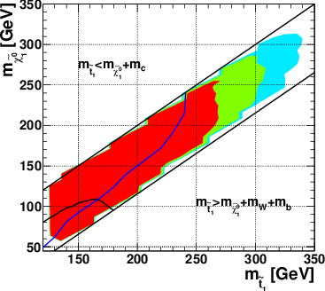
In Figure 10, we show the significance in the stop–neutralino mass plane for an integrated luminosity of $100\,\rm{fb}^{-1}$ at $\sqrt{s}=14$ TeV. We assume the mass relation of Eq. (4). The parameter space below the black curve is excluded by Tevatron searches at the 95% confidence level [27], whereas the parameter points above the blue curve allow detection of a monojet signal with at least $5\sigma$ significance [30]. In our analysis, we assume that the light stop decays dominantly into a charm quark and the lightest neutralino. This will generally not be the the case if the mass relations $m_{\tilde{t}_{1}}>m_{\tilde{\chi}_{1}^{0}}+m_{c}$ and $m_{\tilde{t}_{1}}<m_{\tilde{\chi}_{1}^{0}}+m_{W}+m_{b}$ do not hold.

We first observe in Figure 10 that the significance increases with decreasing stop--neutralino mass difference ⁵⁵ 5 Small deviations from this behaviour are due to statistical fluctuations of the signal.. Recall that we require $p_{T}(b_{1})>150\,\mathrm{GeV}$ . This implies that the $\tilde{t}_{1}\tilde{t}_{1}^{*}$ pair usually has a rather large transverse momentum, which in turn leads to significant boosts of the stop squarks. As a result the charm jets tend to go into a direction close to that of the stop pair; i.e. the charm jets tend to reduce the missing $p_{T}$ . Scenarios with softer charm jets, i.e. smaller $\tilde{t}_{1}-\tilde{\chi}_{1}^{0}$ mass splitting, therefore pass the $\not{p}_{T}$ cut more efficiently. A similar argument also holds for the significance of the monojet signal, where the missing energy is is required to have ${\not p_{T}}>1\,\mathrm{TeV}$ ; moreover, a veto against additional jets is imposed [30].

Our results suggest that a discovery of stops via stop pair production in association with two $b-$ jets is possible as long as $m_{\tilde{t}_{1}}\lesssim 270\,\mathrm{GeV}$ . In the case of non-observation of any signal one would be able to exclude the parameter space at $2\sigma$ for stop masses of up to $340\,\mathrm{GeV}$ ; cf. the turquoise region in Fig. 10. Our signal is also visible in regions of parameter space where the monojet signature produces no significant excess over the SM backgrounds ⁶⁶ 6 We note however that in contrast to our work, Ref. [30] included systematic uncertainties equal to $\sqrt{7B}$ ; see Ref. [30] for more details. The monojet discovery reach will therefore increase if one uses solely $S/\sqrt{B}$ as an estimator for the significance.. This is partly because our process is additionally enhanced by the EW contributions, which do not enter significantly the monojet production process. We note however, that different cuts for the monojet signal than those of Ref. [30] might increase the monojet discovery reach ⁷⁷ 7 We did some estimates for the monojet signal and the most important backgrounds and found that less hard cuts on the monojet $p_{T}$ and on the ${\not p_{T}}$ lead in general to larger significancies. We plan to present our results in a future publication..

IV Possibilities to further optimize the cuts

So far we have only applied cuts that can be used for all combinations of stop and LSP masses, i.e. we have not tried to optimize the cuts as function of $m_{\tilde{t}_{1}}$ or $m_{\tilde{\chi}_{1}^{0}}$ . This simplifies the statistical analysis: if we try several combinations of cuts, the chance of finding an upward fluctuation of the background increases. On the other hand, additional cuts could help to increase not only the statistical significance, but also the purity of the sample, i.e. the signal to background ratio. Note that Table 3 implies a signal to noise ratio of about 0.025 at the limit where the signal becomes statistically significant, i.e. for $S/\sqrt{B}=5$ . If we require $S/B>0.1$ , the search reach would decrease from about 270 GeV to 190 GeV. After imposing the $\tau$ veto, this would improve again to about 200 GeV, which is however still much smaller than the statistical reach.

Recall that our background is dominated by $Zb\bar{b}$ and $t\bar{t}$ events. The systematic uncertainty on the former is very small, since one can analyze events with identical kinematics where the $Z$ decays into an $e^{+}e^{-}$ or $\mu^{+}\mu^{-}$ pair. Of course, $t\bar{t}$ events will also be analyzed in great detail by the LHC experiments; nevertheless some extrapolation into the signal region will presumably be required to determine this background, which will introduce some systematic uncertainty.

Note also that the statistical $5\sigma$ discovery limit after the cuts of Table 3 still corresponds to about $1\,000$ signal events. Refined cuts could therefore also help to further increase the mass reach.

In this section we therefore first discuss some cuts that might help to suppress the $t\bar{t}$ background for scenarios with small $\tilde{t}_{1}-\tilde{\chi}_{1}^{0}$ mass splitting. We then discuss possibilities to identify the $c-$ jets in the signal, which can be used to suppress all backgrounds, and also to distinguish our scenario from other SUSY processes with a similar final state.

IV.1 Further cuts for small mass splitting

If $m_{\tilde{t}_{1}}-m_{\tilde{\chi}_{1}^{0}}$ is small, the $c-$ jets will usually be too soft to be detected. In contrast, many $t\bar{t}$ background events will contain a hadronically decaying $W$ boson in addition to the two required $b-$ jets. We saw in Fig. 7 that this leads to a higher charged multiplicity of these background events. One can cut on several (related) quantities to suppress this background (and, to a lesser extent, the single top background):

•

A jet veto could be imposed. Recall, however, that the signal is almost exclusively due to gluon fusion, which implies strong initial state radiation. In order not to unduly suppress the signal it might therefore be preferable to only veto events that contain two (or more) additional hard jets.
•

An upper limit on the total transverse energy could be imposed; probably the two $b-$ jets should not be included here, i.e. one should only sum over particles (or calorimeter cells) that are not part of these two jets.
•

An upper limit on the charged particle multiplicity could be imposed. For example, requiring $N_{\rm charged}\leq 20$ would reduce the $t\bar{t}$ background by $\sim 30\%$ with little loss of signal.

IV.2 Charm tagging

Observing two soft charm jets in addition to two hard $b-$ jets and large missing energy would give strong evidence for our scenario. However, soft charm jets are probably difficult to identify at the LHC. The underlying event, QCD radiation and possibly overlapping events (which we did not include in our simulation) generate substantial hadronic activity in our signal events and may overshadow potential charm–jets. That said, we can still expect some reasonably energetic $c-$ jets for the light stop scenarios if the $\tilde{t}_{1}-\tilde{\chi}_{1}^{0}$ mass splitting is not too small. For example, for our benchmark point and after applying all the cuts of Table 3 we expect about $45\%$ of all signal events to contain at least one $c-$ jet with $p_{T}>50\,\mathrm{GeV}$ ⁸⁸ 8 Recall that we use $R=1$ in our jet definition. This allows a significant contribution from the underlying event and from unrelated QCD radiation to the jet energy. In the absence of these effects, only $\sim 16\%$ of all signal events contain a $c-$ jet with $p_{T}\geq 50\,\mathrm{GeV}$ ..

Still, we have to discriminate the charm jets from light–flavored and gluon jets. In Ref. [30], the authors use the jet mass and charged particle multiplicity inside the jet to discriminate between $c-$ jets and light flavor or gluon jets. They find $c-$ tagging efficiencies of $\geq 50\%$ for mass splitting $\geq 10\,\mathrm{GeV}$ , but with a 25% mis–tagging probability. In the case at hand it might be better to employ a more sophisticated algorithm, e.g. based on a neural net, that attempts to decide whether the hadronic activity not associated with the two $b-$ jets is consistent with containing two $c-$ jets, rather than identifying the $c-$ jets in isolation.

Identifying at least one $c-$ jet would suppress the $Wb\bar{b}$ , single top and $Zb\bar{b}$ backgrounds. Moreover, it would distinguish the stop pair production we are considering from the pair production of light sbottom squarks ( $\tilde{b}_{1}$ ), followed by $\tilde{b}_{1}\rightarrow b\tilde{\chi}_{1}^{0}$ decays, which also leads to a final state with two $b-$ jets and large missing $p_{T}$ , but without $c-$ jets. However, half of all $t\bar{t}$ events containing a hadronically decaying $W$ boson also contain a $c-$ jet (from a $W^{+}\rightarrow c\bar{s}$ decay or its charge conjugate); $c-$ tagging will therefore probably not be as efficient in reducing the $t\bar{t}$ background.

V Summary and Conclusion

In this article, we analyzed stop pair production in association with two $b-$ quarks in the co–annihilation region, where the $\tilde{t}_{1}-\tilde{\chi}_{1}^{0}$ mass difference is small, so that simple stop pair production does not yield an observable signal. Assuming a light higgsino–like chargino beside a stop NLSP and neutralino LSP, the leading order QCD as well as mixed QCD–EW contributions are taken into account. We discussed in some detail the dominant diagrams for our signal process. We simulated the signal process and dominant SM background processes. For a benchmark scenario with $m_{\tilde{t}_{1}}=120\,\mathrm{GeV}$ , $m_{\tilde{\chi}_{1}^{0}}=100\,\mathrm{GeV}$ and $m_{\tilde{\chi}_{1}^{\pm}}=140\,\mathrm{GeV}$ , we described all important kinematic distributions and developed a set of cuts that help to isolate our signal process. The most effective cut is a veto on isolated leptons. We showed that we can have a significance of $\mathcal{S}=70$ for our benchmark point, assuming an integrated luminosity of $100\,{\rm fb}^{-1}$ at $\sqrt{s}=14\,\mathrm{TeV}$ ; alternatively, a signal with $5\sigma$ statistical significance can be obtained with just $0.5\,{\rm fb}^{-1}$ of data. For fixed $\tilde{\chi}_{1}^{\pm}-\tilde{t}_{1}$ and $\tilde{t}_{1}-\tilde{\chi}_{1}^{0}$ mass differences, the same set of cuts allows to detect the signal at $\geq 5\sigma$ statistical significance for $m_{\tilde{t}_{1}}\lesssim 270\,\mathrm{GeV}$ . Note that the significance of our signal actually increases when the $\tilde{t}_{1}-\tilde{\chi}_{1}^{0}$ mass difference is reduced, making it complementary to searches for direct stop pair production. The inclusion of the EW diagrams greatly enhances the total cross section and more than doubles the statistical significance.

However, we saw that for $m_{\tilde{t}_{1}}>190$ GeV our cuts leave us with a relatively poor signal to background ratio. This can be improved by vetoing $\tau-$ jets, i.e. hadronically decaying $\tau$ leptons. We also briefly discussed additional cuts on the hadronic activity not associated with the two hard $b-$ jets that could help to further suppress the $t\bar{t}$ background, which probably will have larger systematic uncertainties than the $Zb\bar{b}$ background. These cuts should be tailored to the $\tilde{t}_{1}-\tilde{\chi}_{1}^{0}$ mass difference, and perhaps also to the overall mass scale (which affects the amount of QCD radiation); we have therefore not attempted to investigate this systematically. We also briefly discussed the possibility to use charm tagging to further suppress the backgrounds, and to distinguish our process from other SUSY reactions yielding two $b-$ jets and missing $p_{T}$ . Charm tagging, and $\tau$ vetoing, depend quite strongly on details of the detector performance; a quantitative analysis of their efficiency is therefore best left to our experimental colleagues.

One motivation for analyzing this final state is that the mixed QCD–EW production channels might allow to probe the $\tilde{t}_{1}-\tilde{\chi}_{1}^{\pm}-b$ coupling, thereby allowing for the first time to check a SUSY coupling relation involving Yukawa couplings; we intend to investigate the feasibility of determining this coupling in a later publication. This will require that the $\tilde{t}_{1}$ mass is known. Determining both the mass and the EW coupling should be easier if the production of stop pairs recoiling against a photon or a very hard jet [30] also leads to an independent statistically significant signal, which does not depend on the $\tilde{t}_{1}-\tilde{\chi}_{1}^{\pm}-b$ coupling.

Acknowledgements.

We thank Sebastian Fleischmann and Stefano Profumo for helpful discussions. The work of J.S.K. is supported in part by the Initiative and Networking Fund of the Helmholtz Association, contract HA-101 (”Physics at the Terascale”). The work of of S.G. is supported in part by the U.S. Department of Energy, under grant number DE-FG02-04ER41268 and in part by a Feodor Lynen Research Fellowship sponsored by the Alexander von Humboldt Foundation. J.S.K. and S.G. thank the University of Bonn and the Bethe Center for hospitality during numerous visits.

References

[1] H. E. Haber, G. L. Kane, Phys. Rept. 117 (1985) 75; S. P. Martin, In *Kane, G.L. (ed.): Perspectives on supersymmetry* 1, [hep-ph/9709356].
[2] D. S. M. Alves, E. Izaguirre and J. G. Wacker, arXiv:1008.0407 [hep-ph]; H. Baer, V. Barger, A. Lessa and X. Tata, JHEP 1006 (2010) 102 [arXiv:1004.3594 [hep-ph]].
[3] L. E. Ibáñez, C. Lopez and C. Muñoz, Nucl. Phys. B 256 (1985) 218.
[4] M. Carena, G. Nardini, M. Quiros and C. E. M. Wagner, Nucl. Phys. B 812 (2009) 243 [arXiv:0809.3760 [hep-ph]].
[5] M. Carena, G. Nardini, M. Quiros and C. E. M. Wagner, JHEP 0810 (2008) 062 [arXiv:0806.4297 [hep-ph]].
[6] Y. Li, S. Profumo and M. Ramsey-Musolf, Phys. Lett. B 673 (2009) 95 [arXiv:0811.1987 [hep-ph]].
[7] P. Huet and A. E. Nelson, Phys. Rev. D 53 (1996) 4578 [arXiv:hep-ph/9506477]; D. Delepine, J. M. Gerard, R. Gonzalez Felipe and J. Weyers, Phys. Lett. B 386 (1996) 183 [arXiv:hep-ph/9604440].
[8] V. Cirigliano, S. Profumo and M. J. Ramsey-Musolf, JHEP 0607 (2006) 002 [arXiv:hep-ph/0603246].
[9] V. Cirigliano, Y. Li, S. Profumo and M. J. Ramsey-Musolf, JHEP 1001 (2010) 002 [arXiv:0910.4589 [hep-ph]].
[10] K. Nakamura [Particle Data Group], J. Phys. G 37 (2010) 075021.
[11] E. Komatsu et al., arXiv:1001.4538 [astro-ph.CO].
[12] A. D. Sakharov, Pisma Zh. Eksp. Teor. Fiz. 5 (1967) 32 [JETP Lett. 5 (1967) 24] [Sov. Phys. Usp. 34 (1991) 392] [Usp. Fiz. Nauk 161 (1991) 61].
[13] M. B. Gavela, P. Hernandez, J. Orloff, O. Pene and C. Quimbay, Nucl. Phys. B 430 (1994) 382 [arXiv:hep-ph/9406289]; G. R. Farrar and M. E. Shaposhnikov, Phys. Rev. D 50 (1994) 774 [arXiv:hep-ph/9305275].
[14] M. J. Ramsey-Musolf and S. Su, Phys. Rept. 456 (2008) 1-88 [hep-ph/0612057]; J. R. Ellis, J. S. Lee and A. Pilaftsis, JHEP 0810 (2008) 049 [arXiv:0808.1819 [hep-ph]]; Y. Li, S. Profumo, M. Ramsey-Musolf, JHEP 1008 (2010) 062, [arXiv:1006.1440 [hep-ph]].
[15] R. Barbieri and L. Maiani, Nucl. Phys. B224 (1983) 32; J. A. Grifols and J. Sola, Phys. Lett. B137 (1984) 257; C. S. Lim, T. Inami, and N. Sakai, Phys. Rev. D29 (1984) 1488; M. Drees and K. Hagiwara, Phys. Rev. D42 (1990) 1709.
[16] J. R. Ellis, J. S. Hagelin, D. V. Nanopoulos et al., Nucl. Phys. B238 (1984) 453-476.
[17] H. Baer, A. D. Box and H. Summy, JHEP 1010 (2010) 023 [arXiv:1005.2215 [hep-ph]].
[18] K. Griest and D. Seckel, Phys. Rev. D 43 (1991) 3191; J .R. Ellis, T. Falk and K A. Olive, Phys. Lett. B444 (1998) 367 [arXiv: hep-ph/9810360]; M. E. Gomez, G. Lazarides and C. Pallis, Phys. Rev. D61 (2000) 123512 [arXiv: hep-ph/9907261]. C. Boehm, A. Djouadi and M. Drees, Phys. Rev. D62 (2000) 035012 [arXiv: hep-ph/9911496].
[19] C. Balazs, M. S. Carena and C. E. M. Wagner, Phys. Rev. D 70 (2004) 015007 [arXiv:hep-ph/0403224].
[20] G. Belanger, F. Boudjema, A. Pukhov et al., Comput. Phys. Commun. 149 (2002) 103 [hep-ph/0112278]; Comput. Phys. Commun. 174 (2006) 577 [hep-ph/0405253].
[21] H. Baer, R. Dermisek, S. Rajagopalan and H. Summy, JCAP 1007 (2010) 014 [arXiv:1004.3297 [hep-ph]]; K. M. Zurek, Phys. Rev. D79 (2009) 115002 [arXiv:0811.4429 [hep-ph]]; D. Feldman, Z. Liu, P. Nath et al., Phys. Rev. D81 (2010) 095017 [arXiv:1004.0649 [hep-ph]].
[22] M. Kamionkowski and M. S. Turner, Phys. Rev. D42 (1990) 3310; P. Salati, Phys. Lett. B571 (2003) 121 [astro-ph/0207396]; F. Rosati, Phys. Lett. B570 (2003) 5 [hep-ph/0302159]; S. Profumo, P. Ullio, JCAP 0311 (2003) 006 [hep-ph/0309220]; R. Catena, N. Fornengo, A. Masiero et al., Phys. Rev. D70 (2004) 063519. [astro-ph/0403614].
[23] R. Jeannerot, X. Zhang and R. H. Brandenberger, JHEP 9912 (1999) 003 [hep-ph/9901357]; T. Moroi and L. Randall, Nucl. Phys. B570 (2000) 455 [arXiv: hep-ph/9906527]; M. Fujii and K. Hamaguchi, Phys. Lett. B525 (2002) 143-149 [hep-ph/0110072].
[24] K. i. Hikasa and M. Kobayashi, Phys. Rev. D 36 (1987) 724.
[25] C. Boehm, A. Djouadi and Y. Mambrini, Phys. Rev. D61 (2000) 095006 [arXiv: hep-ph/9907428].
[26] V. M. Abazov et al. [D0 Collaboration], Phys. Lett. B 665 (2008) 1 [arXiv:0803.2263 [hep-ex]].
[27] [CDF Collaboration], CDF note 9834.
[28] S. Kraml and A. R. Raklev, Phys. Rev. D 73 (2006) 075002 [arXiv:hep-ph/0512284].
[29] J. Hisano, K. Kawagoe and M. M. Nojiri, Phys. Rev. D68 (2003) 035007 [arXiv: hep-ph/0304214]; S. P. Martin, Phys. Rev. D78 (2008) 055019. [arXiv:0807.2820 [hep-ph]].
[30] M. Carena, A. Freitas, C. E. M. Wagner, JHEP 0810 (2008) 109. [arXiv:0808.2298 [hep-ph]].
[31] A. Freitas and P. Z. Skands, JHEP 0609 (2006) 043 [arXiv:hep-ph/0606121]; A. Freitas, P. Z. Skands, M. Spira and P. M. Zerwas, JHEP 0707 (2007) 025 [arXiv:hep-ph/0703160].
[32] B. C. Allanach, S. Grab, H. E. Haber, [arXiv:1010.4261 [hep-ph]].
[33] S. Bornhauser, M. Drees, H. K. Dreiner and J. S. Kim, Phys. Rev. D 80 (2009) 095007 [arXiv:0909.2595 [hep-ph]].
[34] A. D. Martin, W. J. Stirling, R. S. Thorne and G. Watt, Eur. Phys. J. C 63 (2009) 189 [arXiv:0901.0002 [hep-ph]].
[35] L. Vacavant, I. Hinchliffe, [hep-ex/0005033]; J. Phys. G G27 (2001) 1839.
[36] G. Aad et al. [ The ATLAS Collaboration ], [arXiv:0901.0512 [hep-ex]].
[37] ATLAS collaboration, Early supersymmetry searches in channels with jets and missing transverse momentum with the ATLAS detector, ATLAS-CONF-2010-065
[38] R. Bonciani, S. Catani, M. L. Mangano and P. Nason, Nucl. Phys. B 529 (1998) 424 [Erratum-ibid. B 803 (2008) 234] [arXiv:hep-ph/9801375].
[39] F. Maltoni and T. Stelzer, JHEP 0302 (2003) 027 [arXiv:hep-ph/0208156].
[40] W. Porod, Comput. Phys. Commun. 153 (2003) 275 [arXiv:hep-ph/0301101].
[41] J. Pumplin, D. R. Stump, J. Huston, H. L. Lai, P. M. Nadolsky and W. K. Tung, JHEP 0207 (2002) 012 [arXiv:hep-ph/0201195].
[42] M. Bahr et al., Eur. Phys. J. C 58 (2008) 639 [arXiv:0803.0883 [hep-ph]].
[43] M. Cacciari, arXiv:hep-ph/0607071.
[44] M. Dobbs, J. B. Hansen, Comput. Phys. Commun. 134 (2001) 41-46.
[45] R. Brun and F. Rademakers, Nucl. Instrum. Meth. A 389 (1997) 81.
[46] M. Drees and O. J. P. Eboli, Eur. Phys. J. C10 (1999) 337 [arXiv: hep-ph/9902391]; G. Hiller, J. S. Kim and H. Sedello, Phys. Rev. D 80 (2009) 115016 [arXiv:0910.2124 [hep-ph]].
[47] R. Hauser, Eur. Phys. J. C34 (2004) S173; D. Giordano [CMS Collaboration], Nucl. Phys. Proc. Suppl. 150 (2006) 299.
[48] ATLAS collab., ATL-PHYS-PUB-2009-000.