Stationary, Axisymmetric Neutron Stars
with Meridional Circulation in General Relativity

We use geometrized units for the theoretical computations, where the speed of light $c$ and the gravitational constant $G$ are set equal to unity. The results obtained from neutron star simulations are presented in the more appropriate cgs units. The general relativistic formalism adopts Einstein’s sum convention and is kept as close as possible to the conventions chosen in Gourgoulhon et al. [6]. However, we make a slightly different choice for the range of tensor indices. In our specific choice of coordinates, concrete indices for 4-tensors, 3-tensors and 2-tensors are used as follows:

with the time $t$, the radius $r$, and the angles $\theta$ and $\phi$. Following Misner et al. [7], we choose $\left(-,+,+,+\right)$ as the signature of the metric.

We begin our theoretical considerations by defining a set of physical fields, the so-called basic fields, which determine the state of the neutron star uniquely. Due to the assumption of stationarity and axisymmetry, these and all other fields depend on only two coordinates, the radius $r$ and the polar angle $\theta$. There are two types of basic fields. The first set describes the curvature of spacetime, and its fields are denoted basic geometry fields. The second set are hydrodynamic fields, called basic matter fields, which specify the properties of the stellar fluid. In the following, we will define the basic geometry fields without giving an explanation of how these fields come into being. For that purpose, we refer to Gourgoulhon et al. [6].

The curvature of spacetime is described by the metric $g_{\alpha\beta}$. Using a $\left(2+1\right)+1$ decomposition of spacetime, the ten independent components of the $4$-metric $g_{\alpha\beta}$ are rewritten to new fields in Gourgoulhon et al. [6]. These fields consist of two scalars fields, the $3$-lapse $N$ and the $2$-lapse $M$, two vector fields, the $3$-shift $N^{a}$ and the $2$-shift $M^{m}$, and the $2$-metric $k_{mn}$, respectively:

with the $3$-metric

and

Using a special choice of coordinates, which are denoted as MTCMA (maximal time slicing - conformally minimal azimuthal slicing) in Gourgoulhon et al. [6], these authors write the $2$-metric $k_{mn}$ such that the only non-vanishing components are $k_{rr}=A^{2}$ and $k_{\theta\theta}=A^{2}r^{2}$, where $A$ shall be called the $2$-conformal factor. Adopting the definitions [6]

we then call the eight functions

basic geometry fields. In contrast, for circular spacetimes (i.e. without meridional circulation), only four geometry fields are required.

The neutron star fluid is described by a stress-energy tensor

with the total energy density $\epsilon$, pressure $p,$ and $4$-velocity $u^{\alpha}$. Due to the constraint

the $4$-velocity $u^{\alpha}$ possesses only three independent degrees of freedom. One of them is the specific angular momentum, i.e. the $\phi$-component of

Under our symmetry assumptions (Sect. II.5), the other two degrees of freedom can be expressed in terms of a stream function $\psi$, an approach known to be working fine in Newtonian gravity (equations (2) and (3) in Eriguchi et al. [3]). Further below (Sect. II.5), we will demonstrate that this approach holds in general relativity, too. There, we will also explain how the $4$-velocity $u^{\alpha}$ can be obtained from the stream function $\psi$ and the specific angular momentum $l_{\phi}$. However, by convention we do not call the stream function $\psi$ a basic field, but the modified stream function [3]

So, we refer to

as basic matter fields. Actually, we have chosen the twelve basic fields (5) and (10) in such a manner that they vanish for an empty Minkowski spacetime, which is advantageous for our numerical method.

Each of the basic fields (5) and (10) is specified by a field equation. In this section, we will address the basic geometry fields, which are governed by Einstein’s field equation

where $G_{\alpha\beta}$ is the Einstein tensor. Unfortunately, this equation is written in such a compact manner that it is practically impossible to directly solve for the basic geometry fields (5). Therefore, we use the theoretical consideration of Gourgoulhon et al. [6], who rewrite equation (11) as a set of eight covariant Poisson equations, each of the form

where $\Delta_{{\rm cov}}$, $\Phi$, and $S$ are a covariant Laplacian, a potential, and a source, respectively. In that paper, the covariant Poisson equations are labelled (B3-B7). Trying to validate these equations, we found that the three equations (B3), (B4a) and (B4b) contain minor errors. In Appendix A, we show the corrected versions of these equations.

Let us now have a closer look at the covariant Laplacian $\Delta_{{\rm cov}}$ appearing in equation (12). This operator is the scalar product of two covariant derivatives. Such derivatives can be split into a partial derivative and corrections arising from the curvature of spacetime, expressed in terms of the connection coefficients. In a similar manner, it is possible to express a covariant Laplacian $\Delta_{{\rm cov}}$ in terms of the corresponding flat-space Laplacian $\Delta_{{\rm flat}}$ and curvature corrections. That way, equation (12) can be rewritten as

with some new source $S^{\prime}$. In this way, we arrive at the following flat-space versions of equations (B3-B7) in [6]:

The flat-space Laplacians ${}^{2}\Delta$, ${}^{3}\Delta$, ${}^{2}\Delta_{\;\;\;n}^{m}$ and ${}^{3}\Delta_{\;\;b}^{a}$ are listed in Appendix B, and the rather lengthy sources $S_{\nu}$, $S_{\alpha}$, $S_{\beta}$, $S_{M}^{m}$ and $S_{N}^{a}$ in Appendix I, respectively. Modifying the sources $S_{\beta}$, $S_{M}^{m}$, and $S_{\alpha}$ properly, it is possible to rewrite equations (15-17) such that the Laplacians in these equations act directly on the basic geometry fields $\beta$, $M^{m}$, and $\alpha,$ but not on expressions containing these fields. However, the numerical stability of the fixed point iteration is highly sensitive to such changes, and in that case the iteration would diverge. By experimenting with the GRNS code, we found that the choice made in equations (15-17) produces convergent results.

For rotating neutron stars, we achieved convergence only by setting the source $S_{M}^{m}$ equal to zero on the grid lines adjacent to the rotation axis. Even when increasing the grid resolution, only the adjacent grid lines have to be modified, and thus setting the source equal to zero is a valid procedure.

The basic matter fields (10) are fixed by the equation of state and the equation of general relativistic hydrodynamics

where $\nabla_{\alpha}$ is the covariant derivative. As will become apparent later (Sect. II.7), for a stationary configuration, the equations of hydrodynamics are integrable under the assumption of a barotropic fluid, where the total energy density $\epsilon$ is a function $\epsilon\left(p\right)$ of the pressure $p$ only.

Similar to Einstein’s field equation (11), equation (18) is again too compact to be solved directly. To overcome this problem, we introduce the projector

orthogonal to the $4$-velocity $u^{\alpha}$, where $\delta_{\beta}^{\alpha}$ is the Kronecker symbol. Then, we project equation (18) in the direction parallel and orthogonal to the $4$-velocity:

and bring these two equations in the usual form

which are the energy equation and the general relativistic Euler equation. In the subsequent sections we will extend the Newtonian stream function method [3] to general relativity by a further reformulation of equations (19) and (20).

The stream function $\psi$ is introduced to solve the energy equation (19). In Appendix C, we show that due to our symmetry assumptions equation (19) can be written as the vanishing flat-space $3$-divergence

of the $3$-vector

with [5]

(note that the symbol $\varrho$ is different than the rest mass density $\rho$ introduced later). Then, similar to the Newtonian stream function method [3], equation (21) is automatically satisfied by the relation

This relation reduces two degrees of freedom of the $4$-velocity $u^{\alpha}$ to the one of the stream function $\psi$ (which has the units $[g/s]$). In the Newtonian limit, where $u_{t}=-1$, these two degrees of freedom correspond to the two components $u^{m}$. Unfortunately, in general relativity, the situation is somewhat more complicated, because the components $u^{m}$ together with the third degree of freedom $u^{\phi}$ also appear on the right hand side of equation (24), hidden in the quantity $u_{t}$. However, using equation (24), the constraint (7), and the definition (8) it is straightforward to show that the $4$-velocity $u^{\alpha}$ can still be computed from the stream function $\psi$ and the specific angular momentum $l_{\phi}$.

Taking stationarity and axisymmetry into account, a short calculation shows that the general relativistic Euler equation (20) can be written as

We recall that this equation is a projection orthogonal to the $4$-velocity $u^{\alpha}$ and has thus only three independent degrees of freedom. In the following, we will therefore consider only the three spatial components of equation (25) by setting $\alpha=a$ in that equation. However, we use the temporal component $\alpha=t$, shown in equation (72), to rewrite these spatial components as

Let us start with the azimuthal component of equation (26). For that purpose, we set $a=\phi$ and being aware that all azimuthal derivatives $\partial_{\phi}...$ vanish due to axisymmetry, we obtain

which extends equation (12) of Eriguchi et al. [3] to general relativity. To solve equation (27), we discern the three cases

In case (A), for which equation (27) is satisfied automatically, the neutron star can be differentially rotating, but without any meridional circulation. We are not interested in this case, because it has already been investigated with the RNS code [8, 2, 1]. Case (B) allows a meridional circulation, but not everywhere in the neutron star. In this paper, we do not investigate such solutions nor do we analyze whether they exist at all. Instead, we focus on case (C), where meridional circulation is present everywhere in the star. For that case, we use equation (24) and rewrite equation (27) as

This equation is satisfied by

where $L\left(\psi\right)$ is an arbitrary function of the stream function $\psi$ [9].

We proceed with the meridional components of equation (26), which can be written as

according to Appendix D, where the quantity $w$ is defined in equation (74). This expression extends equations (7) and (8) of Eriguchi et al. [3] to general relativity. Our limitation to a barotropic equation of state allows us to write the left hand side of equation (29) in the form of a gradient. To this end, we introduce the heat function [10]

For the right hand side, we use equations (24) and (28). Then, equation (29) reads

which implies that the right hand side must be a gradient, too, for obtaining a first integral of motion. This leads to the condition

with an arbitrary function $f\left(\psi\right)$. Examining equations (74), (8), and eventually (24), we realize that the quantity $w$ contains second derivatives of the stream function $\psi$. Actually, as shown in the Appendix E, it turns out that there is a Laplacian hidden in that quantity, and that condition (32) is equivalent to

where the modified stream function $\chi_{0}$ (9) is used, and the source $S_{\chi_{0}}$ is given in Appendix I. This flat-space Poisson equation differs from that presented in Sect. II.3 by the appearance of the angle $\phi$.

We now return to equation (31) and insert condition (32). Then, by integration we obtain

with the ancillary function

and the integration constant $C$. The heat function $H\left(p\right)$ appearing in equation (34) is invertible, because the total energy density $\epsilon$ and the pressure $p$ are both positive quantities, and thus also the integrand of equation (30), such that the heat function $H\left(p\right)$ is strictly monotonous. Denoting the inverse heat function as $H^{-1}\left(p\right)$, equation (34) the pressure can be expressed as

with the central pressure $p_{{\rm c}}$, the central stream function $\psi_{{\rm c}}$, and the central covariant temporal component $u_{t}^{{\rm c}}$ of the 4-velocity, respectively. In general, the above inversion is performed numerically.

In Sect. II, we have introduced the basic fields

and their governing equations (13-17), (28), (33), (35) and the equation of state. We solve these equations by means of a fixed-point iteration after having specified an initial guess $\nu_{0},...,l_{\phi,0}$, which is constructed in the following way. We set the basic fields (36) to the Tolman-Oppenheimer-Volkoff solution. This spherically symmetric solution has no meridional circulation, and therefore the basic matter field $\chi_{0}$ vanishes. Then, we modify the Tolman-Oppenheimer-Volkoff solution such that the field $\chi_{0}$ becomes non-zero. For that purpose, we consider surface-adapted coordinates

where $R\left(\theta\right)$ is the radial coordinate of the neutron star surface. Then, the invariance of scalars tells us

and we set

with an arbitrary constant $\chi_{0}^{{\rm max}}$ and parameters ${\cal M}_{r},{\cal M}_{\theta}\in\left\{1,2,...\right\}$, as shown in Fig. 1.

To describe the iteration steps, we denote the values of the basic fields (36) after the $s$-th iteration step by $\nu_{s},...,l_{\phi,s}$, and those after the previous $s$-th iteration step by $\nu_{s-1},...,l_{\phi,s-1}$. The basic geometry fields are then iterated via the equations

where $S_{...,s-1}^{...}$ denotes the sources of equations (13-17) computed from the basic field values $\nu_{s-1},...,l_{\phi,s-1}$. The inverse Laplacians ${}^{...}\Delta_{...}^{...-1}$ appearing above are determined with Green functions according to the detailed description given further below (Sect. III.2). Subsequently we evaluate the source of equation (33) using the newly computed values $\nu_{s},...,M_{s}^{\theta}$ of the basic geometry fields and the old values $p_{s-1},...,l_{\phi,s-1}$ of the basic matter fields, the outcome being called $S_{\chi_{0},s-1}$. Next, we calculate

where $u_{t,s-1}^{{\rm c}}$ is the value of the quantity $u_{t}^{{\rm c}}$ computed from the values of the basic fields $\nu_{s-1},...,l_{\phi,s-1}$.

In the following, we address the inverse Laplacians ${}^{2}\Delta^{-1}$, ${}^{3}\Delta^{-1}$, ${{}^{2}\Delta_{\;\;\;n}^{m}}^{-1}$ and ${{}^{3}\Delta_{\;\;b}^{a}}^{-1}$ appearing in equations (39-44). Each of these inverse Laplacians comes from an equation having one of the forms

where $\Phi^{...}$ and $S^{...}$ are a potential and a source, respectively. To solve for the potential of equation (45), (46), …, we have to compute the first, second, … of the following integrals, shown in the same order as above [5]:

where

for the $2$-dimensional and

for the $3$-dimensional integrals (analogous for $\vec{x}^{\prime}$) together with the Jacobian determinants $\partial\left(...\right)^{a}/\partial\left(...\right)^{b}$. The dots appearing in equation (50) represent additional terms required for the boundary condition of the basic matter field $\chi_{0}$ and are given in Appendix F. In that Appendix, the main focus is on an expansion of the above integrals in terms of trigonometric functions and Legendre polynomials. Typically, only a few terms of the expansions are needed, and neglecting the remaining ones leads to a strong reduction of the computational cost necessary to evaluate the integrals.

According to Gourgoulhon et al. [6], the basic geometry fields $M^{m}$ and $N^{a}$ satisfy the following slicing conditions

where the $2$-and $3$-covariant derivatives ‘$||$’ and ‘$|$’ are defined in Appendix B. A lengthy, but elementary calculation shows that these two slicing conditions can be rewritten as the vanishing flat-space $2$- and $3$-dimensional derivatives

of the quantities

Contrary to an analytic one, a numeric evaluation of the Green functions of Sect. III.2 always produces values for the fields $M^{m}$ and $N^{a}$ which somewhat violate the slicing conditions. Therefore, we consider a $2$- and $3$-dimensional Helmholtz decomposition and set the gradient parts of the two quantities $M_{e}^{m}$ and $N_{e}^{a}$ equal to zero such that the divergences of the remaining parts vanish as demanded by the slicing conditions. Such a procedure is valid, because when the fixed point iteration has converged, the gradient parts (which have to be set to zero) decrease with increasing numerical accuracy, i.e. with increasing grid resolution and number of trigonometric functions and Legendre polynomials used in the integral expansions of the Green functions.

Even now, the basic fields are not yet determined completely. There are still remaining gauge degrees of freedom left, because we can add an arbitrary constant to each of the potentials appearing in equations (45-48) without violating these equations:

For the $3$-dimensional Poisson equations, the Green function

vanishes in the limit $\left|\vec{x}-\vec{x}^{\prime}\right|\rightarrow\infty$. Thus, we choose the potentials of these Poisson equations to vanish at infinity by setting the constant appearing in equation (52) equal to zero. However, for the $2$-dimensional Poisson equations such a choice is not possible, as the Green function

is not bounded for $\left|\vec{x}-\vec{x}^{\prime}\right|\rightarrow\infty$. Therefore, we proceed as follows:

The potential $r\sin\theta\left(\beta+\nu\right)$ of the $2$-dimensional Poisson equation (41) obeys the Dirichlet boundary condition according to Appendix F. Hence, we set the constant in equation (52) equal to zero in this case, which completely fixes the field $\beta$. In case of the $2$-dimensional Poisson equation (40), we choose the constant in equation (52) in such a manner that

For the remaining $2$-dimensional Poisson equation (42), we have to consider only the Cartesian $z$-component $M_{e}^{z}$, because the $x$-component $M_{e}^{x}$ obeys the Dirichlet boundary condition, and we impose the condition

Eventually, we have a closer look at the function $f\left(\psi\right)$ introduced in equation (32). We follow the same approach as Eriguchi et al. [3] and limit ourselves to the power law

with some constant $k$ and the exponent

For the case

we find different meridional circulation modes $\psi_{m}$ (with $m=0,1,2,...\,$), as in the Newtonian case [3]. The distributions of the field $\chi_{0}$ belonging to these modes look similar to the ones displayed in Fig. 1 but are somewhat deformed.

Unfortunately, when nearly having reached one of the higher circulation modes $\psi_{1},\psi_{2},...$ during the fixed point iteration, the fixed point iteration method always starts to converge to the fundamental mode $\psi_{0}$. In order to obtain the higher modes, we therefore projected the lower ones away. For that purpose, we assume that we have already evaluated the first $m_{{\rm e}}-1$ modes, i.e. we know $\psi_{m}$ for $m=0,1,...,m_{{\rm e}}-1$. Then, the fixed point iteration leads to the $m_{{\rm e}}$-th mode by replacing

at every iteration step, with adequately chosen coefficients $C_{m}$. If an orthogonality relation

with the weight function $W_{m}\left(r,\theta\right)$ exists, the coefficients $C_{m}$ are given by

where $h={\rm det}h_{ab}$. However, we neither know whether an orthogonality relation exists nor do we know the weight functions $W_{m}\left(r,\theta\right)$. After some experimenting, we found that the choice

is sufficient to achieve a convergence to higher modes. This does not necessarily mean that (56) is the correct weight function, but it could be very close to it.

In addition to the usage of (56), we perform the following steps in the GRNS code: The pressure distribution of the solutions investigated in this work is always equatorially symmetric. However, in our treatment, equatorial symmetry is not guaranteed exactly due to the limited numerical accuracy. Therefore, equatorial asymmetry may increase during the fixed point iteration, eventually leading to an undesired meridional circulation mode. In order to prevent this, we symmetrize the pressure distribution at every iteration step. A similar method is performed for the basic field $\chi_{0}$, which has either even or odd parity depending on the considered mode.

We have implemented GRNS under Linux in C++, and it possesses an OpenGL visualization interface, which allows the user to supervise the fixed point iteration. The user has full control over the iteration, which can be stopped and restarted at any time. The user can select any of the physical fields either when the iteration is stopped or even when it is running, and display it on the screen. It is also possible to visualize the flow of the neutron star fluid in real time and to see how the neutron star surface changes during the iteration. These code features are of advantage when analyzing the stability of GRNS, and they were also very helpful in debugging the code.

We used a numerical grid of 150 radial and 156 angular zones to compute the models discussed in Sect. IV. For the sums arising from the expansion of the integrals (see Appendix F), we chose the upper limit

where $l_{{\rm max}}=10$ for all models of Sect. IV. This limits the computational cost, and we are able to compute individual circulation modes within about a minute on a current single core CPU. In Appendix G, we discuss the convergence behavior and consistency tests of GRNS.

The results presented in the following were obtained with the usual polytropic equation of state

where $K$ is the polytropic constant, $\rho$ the rest mass density, and $\Gamma$ the polytropic exponent, respectively. From this equation of state its is readily seen that

We keep the maximum absolute value of the stream function $\psi$ fixed at the value $\psi_{{\rm max}}$ such that it does not matter which value we choose for the constant $k$ in equation (53). The fundamental mode of each neutron star model is then unambiguously specified by the following parameters

i.e. by the exponent appearing in equation (53), the central pressure and the central density (which fixes the polytropic constant $K$) of the initial guess, the polytropic exponent, the maximum absolute value of the stream function, and by the distribution (28) of the specific angular momentum. As a reference model, we choose a non-rotating neutron star with parameters

circulating at its fundamental mode. This set of parameters corresponds to a neutron star with the following properties:

The average radius $\bar{R}$ is the average proper radius

averaged over all angles $\theta$ (over all radial paths $C$). We compute the rest mass via [11]

where $V$ is the volume of the star and the average circulation velocity is given by

The basic fields of the reference model are shown in Fig. 2. The $3$-lapse logarithm $\nu$ is one of the two contributions (the other one comes from the 3-shift $N^{a}$) to the time dilation, which is strongest at the center of the neutron star. The $2$-conformal factor logarithm $\alpha$ represents the stretching of space in meridional planes and is also strongest in the center. We do not display the basic geometry field $\beta$ in Fig. 2, because its values are not significantly different from those of the field $\alpha$. The $3$-shift $N^{a}$ represents the dragging of spacetime caused by the flow of the neutron star fluid. Since the reference model is circulating, this leads to the vortex visible in the lower left panel of Fig. 2. The total energy density $\epsilon$ is also not shown in that figure, because it is correlated to the pressure $p$ by the trivial analytic relation (58). Note that in the lower right panel of Fig. 2 the outermost contour is the surface of the neutron star. As the values on the axes of Fig. 2 do not refer to proper but to coordinate distances, the average neutron star radius suggested by the contour is somewhat smaller than the actually correct value (59), which takes the curvature of spacetime into account. The $2$-shift $M^{m}$ and specific angular momentum $l_{\phi}$ vanish for the reference model, because it does not rotate. Instead of considering the modified stream function $\chi_{0}=\psi/\left(r\sin\theta\right)$, we show the stream function $\psi$ itself in the top left panel of Fig. 3, as the contours of the stream function $\psi$ are stream lines of the meridional flow. Note that the stream function of the reference model contains only a single vortex.

The distributions of the $3$-lapse $\nu$, the $2$-conformal factor $\alpha$ and the pressure $p$ given in Fig. 2 do not show any significant difference when compared to the Tolman-Oppenheimer-Volkoff solution used to construct the initial guess for the fixed point iteration. The only relevant changes are that the $3$-shift $N^{a}$ and the stream function $\psi$, which vanish for the Tolman-Oppenheimer-Volkoff solution, display the distributions shown in the lower, left panel of Fig. 2 and the upper left panel of Fig. 3, respectively.

The other three panels in Fig. 3 show higher circulation modes with additional vortices. Actually, each vortex in the stream function $\psi$ is accompanied by a vortex in the $3$-shift $N^{a}$ (not shown for the higher modes). Let us now compare the four modes shown in Fig. 3 with the four initial guesses of Fig. 1. With this in mind, it does not matter that both figures show different fields, because the difference between the stream function $\psi$ and the modified stream function $\chi_{0}$ is merely a factor $r\sin\theta$. Such a factor causes deformations of the vortices, but their number and orientations remain unaffected. Then, it seems as if the top left initial guess of Fig. 1 leads to the top left mode of Fig. 3, and so on. However, there is no such one-to-one correlation. Instead, it can, for instance, occur that the four modes of Fig. 3 are produced by the four initial guesses ${\cal M}_{r}=1$ and ${\cal M}_{\theta}=1,2,3,4$. Actually, it does not matter too much how the initial guesses are chosen. It is only important that they are somehow different, and to improve the fixed point iteration, we have made a choice that is at least similar to the expected outcomes.

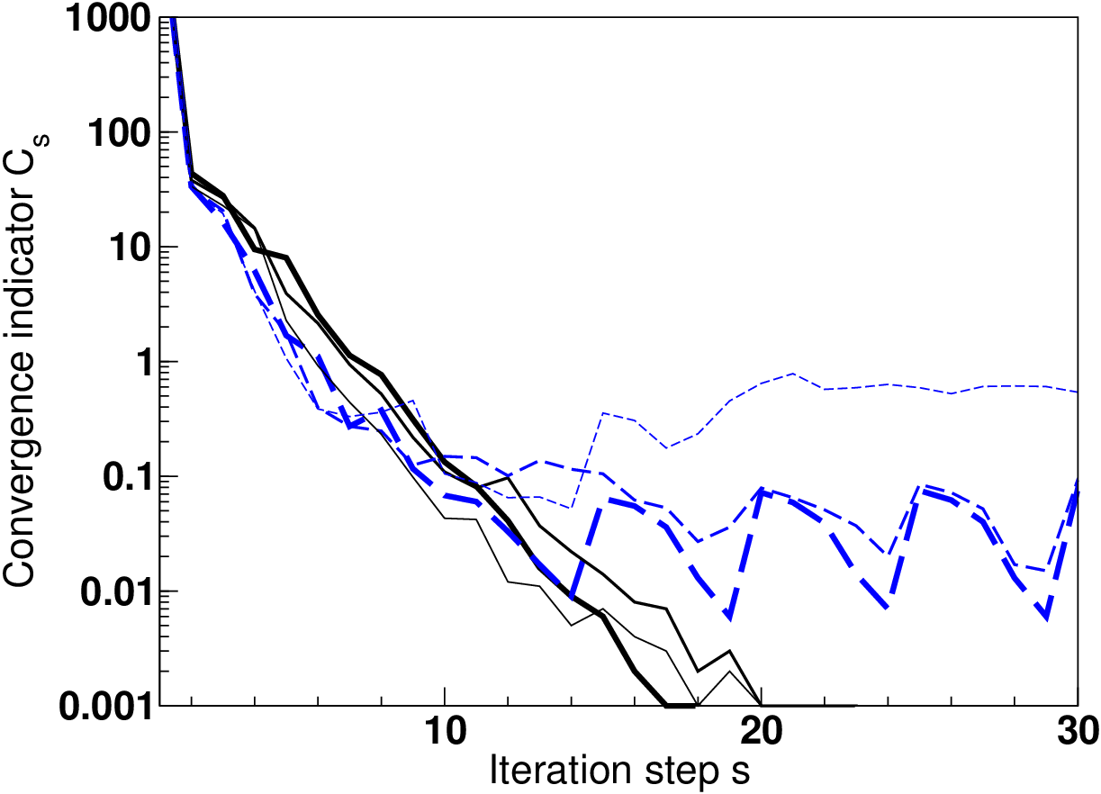
In total, we are able to compute 16 modes for the reference model (including the fundamental mode) before GRNS fails due to too large numerical errors, i.e. we find a much larger set of modes than in Eriguchi et al. [3]. Fig. 4 shows some additional higher modes. The lower right panel of that figure represents the highest mode obtained where numerical errors do not yet have a significant impact on the shape of the vortices. Looking at Figs. 3 and 4, it is obvious that the circulation modes constitute a $2$-dimensional mode set.

A closer look at the surface of the neutron star in Fig. 5 reveals that surface deformations of about half a percent of the average neutron star radius are present. The shape of these deformations depends on the vortices in the vicinity of the surface. Vortices deeper inside of the neutron star have only a small impact on the deformations. In Eriguchi et al. [3], the numerical resolution was too small to resolve such properties. However, it was determined that for the fundamental mode with only a single vortex the meridional circulation causes the neutron star to become slightly prolate.

The strength of the deformations depends also on the velocity of the fluid in the vortices, and thus on the maximum absolute value $\psi_{{\rm max}}$ of the stream function. To test the limits, we increased the value of $\psi_{{\rm max}}$ in GRNS as far as possible. The choice $\psi_{{\rm max}}=3\cdot 10^{34}\,{\rm g}/{\rm s}$ for the reference model is already close to what is possible with GRNS, and we were only able to increase that value to about $\psi_{{\rm max}}=10^{35}\,{\rm g}/{\rm s}$, above which numerical errors grow dramatically. However, even at the limiting value, the surface deformations do not exceed about one percent of the average neutron star radius.

For the choice $\psi_{{\rm max}}=10^{35}\,{\rm g}/{\rm s}$, the average circulation velocity of the reference model is $\bar{v}_{{\rm circ}}=3431\,{\rm km}/{\rm s}$, whereas for a very slowly circulating model with $\psi_{{\rm max}}=3\cdot 10^{34}\,{\rm g}/{\rm s}$ the average circulation velocity is only $\bar{v}_{{\rm circ}}=10\,{\rm km}/{\rm s}$. Actually, it is a good approximation to say that the average circulation velocity $\bar{v}_{{\rm c}}$ scales linearly with the maximum absolute value $\psi_{{\rm max}}$ of the stream function. However, for the average radius and the mass of the neutron star, we do not find any significant changes when the circulation velocity changes, within the range considered here.

Tab. 1 lists the average velocities $\bar{v}_{{\rm circ}}$ of the circulation modes. For that purpose, we use a mode numbering similar to Fig. 1: the first mode number in Tab. 1 gives the number of vortices in $x$-direction, and the second one in $z$-direction. The velocity $\bar{v}_{{\rm circ}}$ obviously increases with the mode numbers, which is a consequence of the orthogonality relation (55). As the average circulation velocity $\bar{v}_{{\rm circ}}$ rises with the maximum absolute value $\psi_{{\rm max}}$ of the stream function, changing the orthogonality relation (55) by inserting an appropriate factor $D_{m}$ in the integrand, it is possible to create new modes with the same velocity $\bar{v}_{{\rm circ}}$, but a different maximum $\psi_{{\rm max}}$. Because it is not easy to determine the factor $D_{m}$, our method is more practical.

Eriguchi et al. [3] investigated both cases (54). Therefore, we now take the reference model and set the parameter $n=0$ such that we obtain

For this case, we do not find a collection of circulation modes but only a single solution, which is shown in Fig. 6. There, we see that compared to the upper left panel of Fig. 3 the stream function is slightly deformed. In addition to that, we find that the average circulation velocity becomes

while the average proper radius $\bar{R}$ and the mass ${\cal M}$ of the neutron star are the same as for the reference model.

In contrast to Eriguchi et al. [3], we have also computed rotating neutron star models with meridional circulation. For that purpose, we set the specific angular momentum $L\left(\psi\right)$ to a non-vanishing value. The simplest choice would be

where the neutron star rotates rapidly near the rotation axis. Eriguchi et al. [3] exclude such models, because the rotation velocity becomes infinite when approaching the rotation axis in Newtonian configurations. In general relativity, the situation is more complicated, because spacetime itself can be dragged by the neutron star fluid. We are not able to present stringent analytical reasons which exclude condition (60), but simulations obeying that condition do not seem to converge for higher numerical resolutions and have to be considered as invalid neutron star models.

Therefore, we consider the next simplest case

For the choice

we find the average circulation and rotation velocities

where the latter is the average value of

When compared to the reference model, the average radius and the mass do not show significant changes, just as most basic fields. Two exceptions are the specific angular momentum $l_{\phi}$ and the $2$-shift $M^{m}$, which vanish for the reference model, whereas for the rotating model (61) their distributions look like as displayed in Fig. 7. They now exhibit a vortex, similar to the stream function $\psi$ and the $3$-shift $N^{a}$. In contrast to the reference model, the $3$-shift $N^{a}$ vector does not only lie within the meridional plane as shown in the lower left panel of Fig. 2, but it has also contributions perpendicular to that plane for the rotating model (not displayed in this paper).

Having investigated model (61), where the circulation and rotation velocities are of the same order of magnitude, the question arises what happens when the rotational velocity is much smaller or much larger than the circulation velocity. Since the reference model itself is non-rotating, we continuously increased its rotation velocity from zero to the value (62) by changing the constant in relation (61). Currently, GRNS fails to compute models where the average rotation velocity is larger than about the value (62). Actually, one would expect that there are at least a few models where the rotation velocity is much larger than the circulation velocity, and possible improvements in the numerical method could allow their computation.

There are not only higher circulation modes for non-rotating configurations, like the reference model, but also for rotating models. In this case, the difference between the fundamental mode and the higher modes is similar to what has been discussed in Sect. IV.2. All of the basic fields containing a single vortex for the fundamental mode, i.e. the four fields $\psi,N^{a},l_{\phi},M^{m}$, exhibit the same number of vortices for a certain higher mode. These vortices are always roughly located at the same spatial position for the four fields. Similar to the non-rotating configurations, the modes where both circulation and rotation are present turn out to be a $2$-dimensional mode collection.

Fig. 8 shows radial profiles of the specific angular momentum (per unit rest mass)

(different from the specific angular momentum $l_{\phi}$, which is defined per unit energy) for the fundamental and one higher mode belonging to the rotating model (61). There, we do not only recognize combined co- and counterrotation, but also that in parts of the star ${\rm dj}/{\rm dr}<0$, which implies that the flow does not satisfy Solberg’s criterion for local stability (see [12] for a proof in GR).

References

• [1] N. Stergioulas and J. L. Friedman, ApJ 444, 306 (1995)
• [2] T. Nozawa, N. Stergioulas, E. Gourgoulhon, and Y. Eriguchi, A&AS 132, 431 (1998)
• [3] Y. Eriguchi, E. Müller, and I. Hachisu, A&A 168, 130 (1986)
• [4] K. Ioka and M. Sasaki, ApJ 600, 296 (2004)
• [5] H. Komatsu, Y. Eriguchi, and I. Hachisu, MNRAS 237, 355 (1989)
• [6] E. Gourgoulhon and S. Bonazzola, Phys. Rev. D 48, 2635 (1993)
• [7] C. W. Misner, K. S. Thorne, and J. A. Wheeler, Gravitation (San Francisco: W.H. Freeman and Co., 1973)
• [8] N. Stergioulas, T. A. Apostolatos, and J. A. Font, MNRAS 352, 1089 (2004)
• [9] I. W. Roxburgh, Ap&SS 27, 425 (1974)
• [10] S. Bonazzola, E. Gourgoulhon, M. Salgado, and J. A. Marck, A&A 278, 421 (1993)
• [11] G. B. Cook, S. L. Shapiro, and S. A. Teukolsky, ApJ 398, 203 (1992)
• [12] F. H. Seguin, ApJ 197, 745 (1975)
• [13] R. A. D’Inverno, Introducing Einstein’s relativity (New York: Oxford University Press, 1992)