Convergence Speed of the Consensus Algorithm with Interference and Sparse Long-Range Connectivity
Abstract
We analyze the effect of interference on the convergence rate of average consensus algorithms, which iteratively compute the measurement average by message passing among nodes. It is usually assumed that these algorithms converge faster with a greater exchange of information (i.e., by increased network connectivity) in every iteration. However, when interference is taken into account, it is no longer clear if the rate of convergence increases with network connectivity. We study this problem for randomly-placed consensus-seeking nodes connected through an interference-limited network. We investigate the following questions: (a) How does the rate of convergence vary with increasing communication range of each node? and (b) How does this result change when each node is allowed to communicate with a few selected far-off nodes? When nodes schedule their transmissions to avoid interference, we show that the convergence speed scales with , where is the communication range and is the number of dimensions. This scaling is the result of two competing effects when increasing : Increased schedule length for interference-free transmission vs. the speed gain due to improved connectivity. Hence, although one-dimensional networks can converge faster from a greater communication range despite increased interference, the two effects exactly offset one another in two-dimensions. In higher dimensions, increasing the communication range can actually degrade the rate of convergence. Our results thus underline the importance of factoring in the effect of interference in the design of distributed estimation algorithms.
Keywords–Average Consensus, Wireless Networks, Scaling Laws, MAC Protocols.
I Introduction
I-A Motivation
The advent of wireless sensor and ad hoc networks has motivated the need for distributed information processing algorithms, which allow each node to operate only on local information. A well-studied algorithm that allows distributed averaging is the average consensus algorithm, wherein the global average of a set of initial sensor observations can be computed based on purely local computations at each sensor. Starting from a set of initial measurements, the average consensus algorithm allows a set of nodes to communicate by a (possibly time-varying) topology to iteratively compute the global average of the initial measurements, see e.g., [1, 2, 3, 4, 5, 6, 7, 8, 9] and references therein. The connectivity properties of the topologies that ensure convergence have been well-studied (e.g., [10, 11]). Of late, the focus has shifted to studying convergence in the face of communication constraints, like quantization [12, 13, 14], packet drops [15] and noise [16]. A closely associated algorithm is the gossip algorithm [17, 2, 18]. In particular, the recent work [18] proposes and studies a probabilistic version of the broadcast gossip algorithm [17]. The idea is to exploit channel fluctuations to enable opportunistic longer-range message-passing. Since only one node is allowed to transmit at any given time, the question of interference does not arise.
In this paper, unlike prior work, we study the effect of interference, which becomes important in the formation of more general message-passing topologies. We explicitly model the effect of interference on the rate of topology formation—and hence convergence—of the average consensus algorithm. This important effect—which crucially depends on network geometry—has been largely ignored. In wireless networks, depending on the physical proximity of to and to , the transmission from to and to may interfere with one another; hence two time slots may be needed to establish edges and . The network thus has two time-scales of interest: that of establishing individual communications among the desired set of nodes and that of the iterations of the distributed algorithms, which occur only when all the desired nodes have successfully communicated. One may thus, view the underlying communication network as constructing the desired message passing graphs from several feasible sub-graphs, each of which satisfies half-duplex, fading and interference constraints. The union of all these sub-graphs is the desired message passing graph.
To illustrate this, consider the formation of a simple linear 6-node network shown in Fig. 1. Suppose the estimation algorithm requires nearest-neighbor communication (shown as bidirectional edges). However, due to interference constraints, only every third node can transmit. In this case, we see that forming the the desired topology requires at least three time-slots, as shown. In other words, for these interference constraints, this topology’s fastest rate of formation is three time slots. Clearly, a topology’s intrinsic benefit and the fastest rate of its formation determine its true utility.
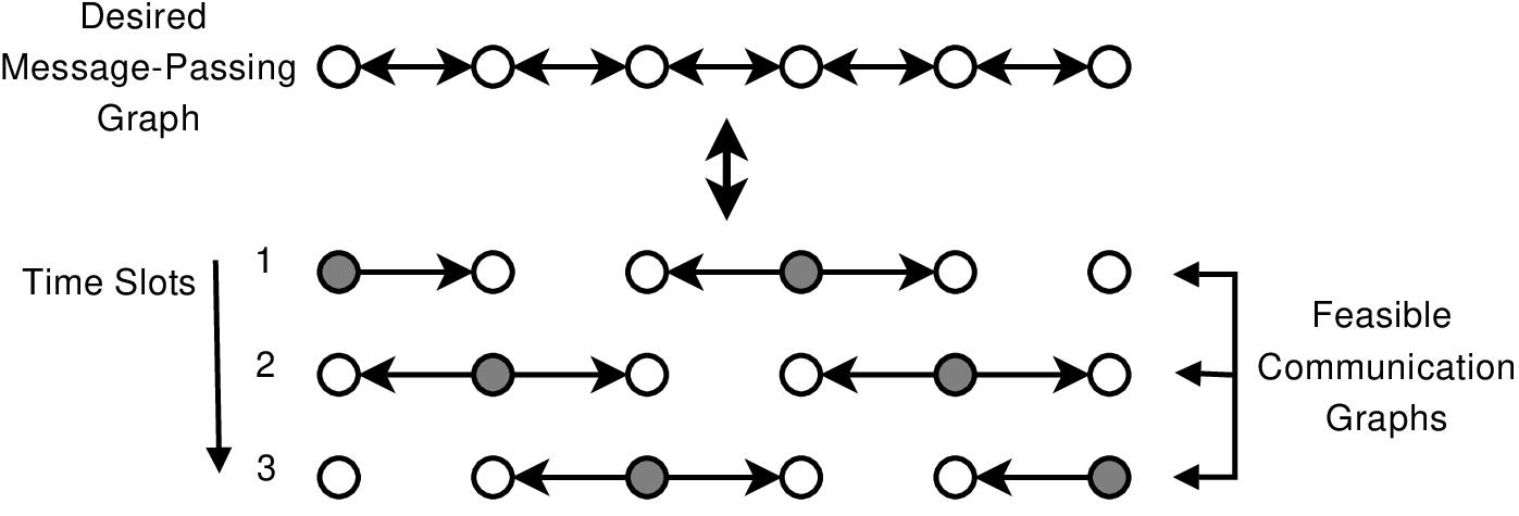
The performance of the underlying (real-time) estimation algorithm is therefore coupled with algorithms for channel access and routing. In our previous work [19], we studied the coupling with channel access for the average consensus algorithm for a certain class of deterministic network topologies. Using a simple protocol model [20] for reception, we were able to show that the effect of increasing network connectivity depends crucially on its dimension. In our recent work [21] we exploited the well-known parallels between the convergence of the average consensus algorithm and Markov chain mixing (e.g., [2] and the references therein) to study consensus on disk graphs [22] using the more refined physical model. We examined the scaling behavior of the fastest rate of topology formation with interference, captured by the shortest feasible TDMA schedules that construct the graph.
We note here that implementing inter-node communication in a network will require some additional overhead. For example, one possible protocol that establishes point-to-point communication can have nodes tag their packets with their uniquely assigned address. A receiver reads this address and decodes a packet only if the address is that of one of its intended transmitters. In this work, we neglect this additional overhead. However, we show that even when this overhead is neglected, increased interference alone is enough to significantly lower the rate of topology formation.
I-B Main Contributions
In this paper, we study networks with short-range and networks with both short-range and limited long-range communication. Although remarkable improvements in convergence rate have been reported [23, 24, 25] for consensus on graphs with a few long-range edges (as in small-world graphs [26]), it is not clear if these benefits will carry over to a wireless setting, where long-range links come at a cost of increased interference. Motivated by this fact, we study the average consensus problem in graphs formed by overlaying long-range edges onto an existing “short-range” disk graph. We derive the scaling law for the spectral gap as well as that of the fastest rate of topology formation in the presence of interference. To the best of our knowledge, this is the first such attempt.
We find that the spectral gap scales quadratically in the communication range , independently of the network dimension , but the length of the shortest TDMA schedule that constructs such graphs scales as . Thus when interference is factored in, the benefit of a greater communication range depends crucially on the network dimension:
- •
For one-dimensional networks (), topologies with increased communication range can converge faster despite greater interference.
- •
For two-dimensional networks, the rate of convergence scales independently of the communication range.
- •
For three- (and higher-) dimensional networks, increasing the communication range can actually slow down convergence.
Furthermore, these results hold whether each node only communicates with all other nodes within its communication range, or, additionally, with a small number of far-away nodes. Thus our results significantly change many optimistic results obtained by analyzing the consensus problem in an abstract graph-theoretic setting.
The remainder of this paper is organized as follows. In Section II, we provide some standard definitions and results used in this paper. In Section III, we specify our system model and formulate the problem using the terminology developed in Section II. In Section IV, we discuss convergence results for the disk graph model. In Section V. we study the effect of selective long-range communication and provide the relevant scaling results. Section VI concludes the paper.
II Definitions and Notation
To make this paper self-contained, we formally state the following standard definitions and facts about Markov chains and introduce some notation and other relevant terminology.
II-1 Basic Definitions from Markov Chain Theory
Consider a connected undirected graph , with vertices and a set of edges . We assume also contains all self-loops, i.e., . Let denote the degree of vertex . For more information, see [27].
Definition 1.
(Random walk on a graph) A random walk on is characterized by the transition probability matrix , with , and only if , with .
Observe that is stochastic.
Definition 2.
(Symmetric random walk) A random walk is symmetric if .
For a symmetric random walk is doubly stochastic.
Fact 3.
A random walk on is a Markov chain with state space . Given an initial distribution over , the distribution after steps satisfies for
Definition 4.
(Stationary distribution of a Markov chain) A stationary distribution satisfies , i.e., remains invariant with time.
Definition 5.
(Reversible Markov chain) A Markov chain is said to be reversible if for all states , .
Fact 6.
An irreducible and aperiodic Markov chain has a unique stationary distribution.
Definition 7.
(Natural random walk) A natural random walk on is a random walk with
Fact 8.
The natural random walk is reversible, irreducible and aperiodic with a unique stationary distribution When is regular, a natural random walk is also symmetric and has a uniform stationary distribution.
Definition 9.
(Mixing time of a random walk) For a random walk with a unique stationary distribution , consider the Total Variational (TV) distance11 1 The TV distance between two distributions and over a countable set is defined as (essentially the norm). (cf. [27, Chap. 4]) for an initial distribution . Then the mixing time of is defined as
II-2 Asymptotic Notation
We use the following asymptotic notation. For two functions and of a variable , as , we write
- •
if the ratio is asymptotically finite. Further, if this limit is zero.
- •
if . Further, .
- •
if and .
When and are random, these relations are defined to hold with probability one.
II-3 Graph Sequences and the Asymptotic Regime
Consider a sequence of (possibly random) undirected graphs , whose member has vertices and a set of edges . We assume each graph contains all self-loops. Denote the maximum and minimum node degrees of by (shortened to ) and (shortened to ) respectively. We provide some standard definitions below.
Definition 10.
(Asymptotically regular graph) is asymptotically regular if .
Definition 11.
(Asymptotically almost sure validity) A property is true asymptotically almost surely (a.a.s.) for a sequence of random objects , if .
We obtain scaling results for the convergence of the average consensus algorithm in large networks by mapping the problem to the scaling of mixing times of natural random walks on a sequence of graphs that are connected and regular asymptotically almost surely.
III Problem Formulation
III-A Average Consensus and Random Walks
Consider a set of sensor nodes . Associate with the sensor an initial observation . Given a realization of a random message-passing graph with vertices and edges , suppose that all the vertices synchronously update their observations as
| (1) |
Here denotes the neighborhood of vertex in . By stacking the individual observations to form the observation vector , the update starting from an initial observation vector can be written as
| (2) |
where we have defined the update matrix , where denotes the identity matrix, and is the graph Laplacian. Notice that depends on the realization of the random graph , which remains the same for all iterations. We will analyze the speed of convergence for specific families of random graphs in the scaling limit , by deriving properties of interest that hold a.a.s. for all realizations of .
Without loss of generality, let , and define as the normalized initial observation vector. In the light of Fact 3 and Definition 7, the iteration can now be interpreted as time-evolution of the node occupancy distribution of a natural random walk over with a transition probability matrix [2, 23].
If is also connected, this equivalence with a natural random walk ensures (from Fact 6) that the value of each vertex asymptotically reaches (a more general result for a time-varying case was studied in [10]). Interpreting each vertex as a sensor and the initial values as sensor measurements, this algorithm allows each sensor to iteratively compute the average of the initial measurement set by exchanging messages as described in (1). We will sometimes also refer to as the message-passing network.
The rate of convergence of (2) to its steady state value can be understood in terms of the mixing time of the natural random walk described by . Indeed, by expressing in terms of , we can write from Definition 9:
| (3) |
where .
When is a.a.s. connected and regular, we know from Fact 8 that the stationary distribution of the random walk is uniform a.a.s., thereby implying convergence to average consensus a.a.s.
In this paper, we analyze random graphs based on the disk graph [22], which are parameterized by the disk radius (see Section III-B). For this family of graphs, it is well-known that the graphs are a.a.s. connected if and only if the radius remains large enough with (i.e., in the “supercritical” regime [28], see, e.g., [29] for a proof). In this regime, the asymptotic regularity property was formally shown to hold a.a.s. in [2, Lemma 10]. In fact, in [2] these two properties were used to establish scaling laws for the mixing time of both the natural and the fastest mixing reversible random walks on these graphs to the uniform distribution.
It is well-known that the mixing time of a random walk can be characterized by the second-largest eigenvalue of . Denoting the eigenvalues of by , the asymptotic convergence of the iteration (2) is determined by . The result below formally establishes this dependence:
Theorem 12.
[30]. The mixing time of a random walk with a doubly stochastic positive definite transition matrix on a connected graph is bounded as
where is called the spectral gap of .
Remark: Observe that the spectral gap controls the mixing time. In the scaling limit , the scaling of also becomes important. The logarithmic dependence on suggests three meaningful possibilities:
- 1.
Polynomial scaling: for some fixed .
- 2.
Exponential scaling: for some fixed .
- 3.
Constant error: is constant.
For polynomial and exponential error scaling, it is clear that the bounds in Theorem 12 are of the same order, and are and respectively. For constant error, the upper bound scales times faster than the lower bound, i.e., and .
In the sequel we assume polynomial scaling, as was done in [2]. It will become clear in the later sections that the scaling laws for exponential scaling follow from a substitution .
Spectral Gap and Cheeger’s Inequality:
Intuition suggests that the mixing time of a Markov chain depends on how “easy” it is to move out of any specified region in the state space. This property can be formalized with the notion of conductance. The conductance of a reversible Markov chain on a state space on a graph with an equilibrium distribution is defined as follows [31]:
| (4) |
where and , and . Viewed in graph-theoretic terms, the numerator (4) measures the effective weighted flow across the cut , while the denominator measures the weighted capacity of . Intuitively, we would expect a larger conductance to correspond to a smaller mixing time, or equivalently from Theorem 12, a larger of the underlying graph . This is indeed the case, as Cheeger’s Inequality shows:
Theorem 13.
[30]. The spectral gap of a reversible Markov chain satisfies
where is the conductance of the Markov chain.
Once we know how scales with for a (random) sequence of graphs , we can use Theorem 13 to find the scaling law for their spectral gap. This, in turn, permits the use Theorem 12 in deriving scaling laws for the mixing time for iterations of the form (2) on these sequences of graphs. In the following, motivated by the need to capture the distance-dependence and randomness in the connectivity of the nodes, we present random geometric graph models for .
III-B Network Models
Each point is placed uniformly randomly in a dimensional torus on , i.e., the vertices form a binomial point process [32] , , on . Each element of is based on the well-known disk graph model [22, 28]. In the following let denote a Euclidean ball centered at and radius , and denote its volume.
III-B1 Networks with Short-Range Communication
In this case, is the dimensional disk graph parameterized by the common communication range of each node. The neighborhood of node that will be used for implementing (1) is
where denotes the Euclidean norm. In this paper, we will always operate in the super-critical regime, i.e., , where to ensure asymptotic connectivity and regularity of [20]. We label this family of graphs as , and the update matrix by . We refer to the points of either by their location or by their index .
III-B2 Networks with both Short- and Selective Long-Range Communication
We start with a disk graph and add long-range edges of length . The parameter controls the distance over which long-range communication occurs: for a given a node can communicate with nodes farther away as . We add the long edges as follows.
For some and , tile the torus with hypercubes of side length . Let denote one of these hypercubes. Along each dimension , let and denote the farthest hypercubes from that are less than distance away from along the coordinate axis, the distance being measured in terms of the separation between their farthest edges. We call these hypercubes as the partner hypercubes of . Figure 2 illustrates the case of . It is easy to see that from any vertex in , any vertex in and is at a distance of at most for a small enough .
Since , every tile contains nodes a.a.s. Without loss of generality, let be one of these nodes. Now add an edge between and every vertex in for . Thus each of these nodes becomes a long-range partner of . Repeat this procedure for every node in , and count duplicate edges only once. Thus for , every node in every tile is additionally connected to nodes a.a.s., i.e., is regular asymptotically almost surely. Hence an iteration of the form (2) on this graph will converge to a uniform distribution a.a.s. We define the resultant graph as and the corresponding update matrix by .

Notice that this model adds long edges selectively to each node; it is motivated by the observation that a small number of long edges added to a graph can greatly increase its spectral gap, as is the case in small-world graphs (cf. [33, Chap. 14]). We have adapted this idea to a wireless network. Instead of adding a single additional edge to a node as is normally the case in abstract graph-theoretic models, the inherent broadcast nature of the wireless channel allows a transmitter to broadcast its information to several receivers that are in close proximity to one another with very little overhead. This allows multiple communication paths to form simultaneously.
We now describe the communication model, which is a well-accepted model in the study of wireless networks.
III-C Communication Model
We make the following assumptions on the communication model:
- •
All edges in and are established by wireless links that operate in the same frequency band (normalized to unit bandwidth).
- •
Each node encodes its message in nats, such that there is negligible quantization error. These messages are sent using a point-to-point capacity-achieving AWGN channel code with SNR threshold (i.e., ). Transmissions are slotted with channel uses allowed per slot.
- •
There is no fading. The path-loss exponent is greater than the dimension of the network, so that the interference remains finite a.s. as the network size grows.
- •
A packet from node can be received at iff the Signal-to-Interference-Ratio (SIR) at node , , is greater than a known constant . Therefore for any sender and receiver , the link will be in outage iff
(5) where is the set of all senders that transmit in the same slot as . This is the well-known interference-limited physical model [20]22 2 It is possible to derive our scaling results by including both noise and interference in the SINR model at the cost of making equations and derivations more cumbersome while distracting from the main message of the paper, which is the analysis of the performance with interference. Hence we focus on the interference-limited case..
- •
The medium-access scheme is TDMA with spatial re-use.
Thus the successful formation of each edge in a graph is mapped to a successful link formation in each direction. Notice that (5) models that fact that there is a limit to the number of edges that can be formed simultaneously, and consequently on the maximum rate at which a given message-passing graph can be established. For a given TDMA protocol, the rate of topology formation is thus determined by its schedule length in time-slots. Since we investigate networks in the scaling limit, we will investigate the scaling properties of the fastest TDMA protocols that can establish a given sequence of random graphs (i.e., have the smallest schedule length a.a.s.)
III-D Quantifying the Effective Speed of Convergence
Note that the mixing time, which is a function of the update matrix , the smallest number of iterations to converge to an ball around the average consensus point. This is different from the time taken to taken to converge to this ball with a finite rate of topology formation in each iteration. For example, in Fig. 1, due to interference constraints, the shortest schedule to construct this topology has at least three time slots. Hence message-passing iterations using this topology can occur no faster than once in every three time slots.
Thus for a topology and an update matrix , the smallest effective time to converge is the product of the mixing time of a topology and the length of the shortest TDMA schedule that constructs the topology in each iteration. We call this the Slot Mixing Time. We formally state it below for future reference:
Definition 14.
(Slot Mixing Time) The Slot Mixing Time is defined as the product
where is the mixing time of iterations using a message-passing graph and an update matrix and is the length of the shortest TDMA schedule that constructs in time slots.
Notice that in general depends on the realization of the random graph . We will analyze the scaling of for the families of random geometric graphs described in Section III-B.
III-E Asymptotic Behavior
IV Convergence in Networks with Small Communication Range
IV-A Characterizing the Spectral Gap
The spectral gap for the disk graph is known to be , independent of network dimension [2]. Using Cheeger’s Inequality (Theorem 12), it was shown that the mixing time of the fastest mixing reversible random walk with a uniform distribution on , for polynomial scaling , scales as
| (6) |
It was also shown therein that the mixing time for the natural random walk on is also . We will now use combine the scaling law for the mixing time with the fastest rate of topology formation implied by the communication model in Section III-C.
IV-B Interference-Limited Topology Formation
We now prove two results that follow from the assumptions made in Section III-C.
Proposition 15.
Consider a system of nodes on a dimensional torus with a short-range communication range , that communicate using point-to-point codes with SINR threshold , with being the path-loss exponent. Assuming the short-range network model in Section III-B1 and the communication model described in III-C, the length of the shortest TDMA schedule that constructs has no fewer than slots a.a.s., for some positive constant .
Proof.
Let be the set of concurrent transmitters at any given time. Suppose node is an intended receiver of a transmitter . Then ’s message is decoded correctly iff (5) is satisfied. Thus for all ,
| (7) |
Clearly this is true even for the farthest intended receiver. It is easy to show that such a receiver lies a.a.s. in a ring of inner radius for some fixed . We thus conclude a.a.s.
This suggests that any TDMA protocol allowing to pass a message to its farthest node needs to set up a guard zone of radius no smaller than around . Since every node inside this guard zone must transmit at least once to form the required message passing graph, any TDMA protocol that constructs the message passing graph requires least slots. Here the indicator is used to indicate the existence of the point inside the ball . The summation is over all points .
For , each such ball has a.a.s., where . ∎
Proposition 16.
Proof.
The proof involves construction of a feasible TDMA schedule whose length is Let for some fixed . Consider the lattice that consists of points on the scaled integer lattice that also lie on the torus. In other words, . Partition into sublattices as follows:
- •
- •
- •
- •
With each lattice site one can associate the tile that lies within the torus . Denote by the set of such tiles associated with each of the points in , . For example, . Thus partition the torus .
The idea behind such a partition is to enable spatial re-use. Consider the following four-phase MAC protocol consisting of phases 00, 01, 10, 11. In phase at most one node from each tile in is allowed to transmit. The protocol ensures that each node transmits exactly once.
The next step is to show that this protocol provides the desired connectivity to each node every time slots for some positive . To this end, we first show that the interference at each intended receiver is bounded from above and can be made smaller than any by a suitable choice of .
Consider one such transmission in phase 00. Let be the set of all transmitters. Consider a transmitting node in tile where , i.e., a tile at the origin. To remain feasible, the protocol must satisfy (5) for each successful link. For any , it is clear that
since . Therefore for a transmitter at , the interference power at any intended receiver at can be upper bounded as
| (8) |
where the right hand side is independent of . By the design of the protocol, an interferer for any intended receiver of the message from must lie in a tile distinct from . Moreover, such a tile should lie within ; thus the protocol imposes a lower bound on the minimum distance between any two concurrent transmitters. Using geometrical arguments (see Figure 3), the right hand side of (8) is upper bounded as
| (9) |

for some fixed , since the sum converges for (in general, for , as assumed in the communication model). The SIR condition (5) is guaranteed to be satisfied at every intended , if is chosen such that
For a suitable choice of , we can set .
For , the number of nodes in each tile is a.a.s. Hence as , the protocol constructed requires transmissions almost surely to establish the necessary connectivity to each node in the network, where . By optimality, the number of slots in the shortest TDMA schedule cannot exceed this number. ∎
Corollary 17.
If denotes the length of the shortest TDMA schedule, then as , a.a.s.:
- 1.
For fixed , .
- 2.
When , .
Proof.
Since (but not ) is independent of , we can write for , when .∎
If all nodes had independent point-to-point channels between one another, the rate of topology formation would be . For a wireless channel, however, Corollary 17 suggests that it requires even with optimum spatial re-use. Thus better-connected disk graphs are penalized by a smaller rate of topology formation. We combine the mixing time result (6) to examine the scaling law for the effective time necessary for convergence in the next section.
IV-C Rate of Convergence
IV-C1 Slot Mixing Time
We now analyze the asymptotic convergence behavior of the distributed averaging algorithm (2) in a dense network as . From the earlier sections, we know the scaling laws for this regime for:
- 1.
The number of iterations necessary to a.s. reach an ball (from (3)).
- 2.
The shortest TDMA schedule length to a.s. realize in each iteration (from Corollary 17).
Thus from Definition 14, for fixed , the Slot Mixing Time scales as
| (10) |
slots a.a.s., for .
From Proposition 15 and the Gaussian signaling assumption, when we also allow to depend on such that , the time to reach this ball scales as
where .
IV-C2 Choice of Communication Range
For a fixed the mixing time in (10) scales polynomially in for . Interestingly, for , the time slots to mix scales as the inverse of . This suggests that increasing can improve the rate of convergence. For , however, this quantity scales independently of , suggesting that these two effects exactly cancel each other, a rather non-intuitive result. For higher dimensions, the scaling law has a positive exponent in —implying that the increasing can actually slow down mixing.
This dependence on network dimension can be understood as follows. If the network is one-dimensional, although a transmitter is an isotropic radiator, its effect on the network is seen only along the line . Although the throughput provided by the optimal TDMA protocol only scales as for a given from Corollary 17, the spectral gap scales as , offsetting this loss. In dimensions, however, while the the fastest rate of topology formation scales as , the spectral gap only scales as . As a result, improving spatial re-use can become more important than increasing connectivity.
IV-C3 Effect of Increasing Transmission Rate
On the one hand, higher transmission rate reduces the packet transmission time; on the other, it also restricts spatial re-use. Clearly the benefit of smaller packet transmission times can be outweighed by reduced spatial re-use for large rates .
V Convergence in Networks with Selective Long-Range Connectivity
V-A Scaling of the Spectral Gap
To derive the scaling law for the mixing time, we need to find the scaling of the spectral gap of . As we will see, deriving the scaling law for the conductance of is sufficient to establish the scaling of the spectral gap.
Proposition 18.
The conductance of with edge weights determined by is a.a.s., for
Proof:
We adopt a modified version of the proof in [34]. From (4) we know that
By the symmetry in induced by the construction in Section III-B2, it can be shown using arguments similar to [34, Appendix G] that the minimum occurs for , and that the minimizing cut is a hyperplane dividing the torus into two halves. Without loss of generality, define .

Also for the natural random walk, each edge weight is (for dimensions, ), and the equilibrium distribution is . It is thus sufficient to count the number of edges traversing this cut. The number of short edges was shown in [34] to be (for dimensions ). Observe that every node in a square of side has long-range partners. One quarter of these edges traverse the cut ; hence the potential number of long edges that can traverse the cut from a given square is . Since each edge has length at least (since and ), which is at most , it is clear that squares from the cut will contribute to the edges that traverse the cut (see Fig. 4). Multiplying this result by the number of rows of such squares, the total number of long edges traversing the cut will be (for general , ). Counting both the short and long edges, we have in dimensions,
since .
Notice that if a node were allowed to have only a finite number of long-range partners, the contribution of long-edges towards conductance is smaller, without significant interference-reducing benefits. We elaborate on this point in Section V-C3. ∎
We can infer the following from the above result:
Corollary 19.
The spectral gap of is and .
Proof:
From the lower bound in Theorem 13, we have . From the upper bound from the same theorem, we have .∎
As noted in Section III-B2, the distance between any two (graph-theoretic) neighbors is no more than . Thus every edge in is also present in the disk graph , i.e., . Hence a reversible random walk on with a uniform equilibrium distribution can mix no faster than the fastest mixing such random walk on . This key observation allows us to use a known result that follows from [2, Thm. 8]:
Theorem 20.
The spectral gap corresponding to the transition probability matrix of the fastest mixing reversible random walk on with a uniform equilibrium distribution is a.a.s.
Since mixing time decreases with spectral gap, from Theorem 20 we conclude that the spectral gap of is . But we know from Corollary 19 that this gap is also . Thus we conclude that the spectral gap of is , which is formally stated as a theorem:
Theorem 21.
The spectral gap of the natural random walk on is .
This result suggests that the improvement in spectral gap from an increased communication radius from to can also be achieved (in the scaling sense) by allowing each node to communicate with a selected number of nodes at a distance .
However, as we shall discuss in the next section, such connectivity comes at a price of a lowered rate of topology formation. We find that this loss (as measured by the shortest TDMA schedule length) must be no smaller than the number of nodes in the largest exclusion zone created in the network. Since the longest link distance in both the disk graph and are of the same order, the similarity in the expressions for the spectral gap scaling law suggests that we should expect the same dependence on network dimension as in (10).
V-B Convergence with Interference
We will derive bounds for the shortest feasible TDMA schedule for . In the spirit of the earlier proofs, the lower bound follows from the feasibility constraint (i.e., the schedule constructs the desired message passing graph while satisfying the SINR constraint), while the upper bound is found by bounding the length of the optimum schedule by that of a specific feasible schedule. These results are presented in the following.
Proposition 22.
For a given , a feasible schedule for has slots a.a.s. for some positive constant . Furthermore, for a given , this length scales as slots a.a.s.
Proof:
We prove this result for ; the proof for is similar. From the system model, it is clear that a TDMA protocol that constructs must form at least one link of distance at least . Since (i.e., scales “much slower” than ), at large enough , the protocol must create an exclusion zone of radius of at least in the network at least once. All nodes within this exclusion zone must transmit at least once. But , which implies we operate the supercritical regime. From a similar argument as in Proposition 15 we can assert that any feasible TDMA protocol must have at least slots where is a positive constant. The scaling law for this length follows from the scaling of with .∎
Proposition 23.
For a given , the length of the shortest feasible schedule for is no more than slots a.a.s., for some positive constant . For a given , this upper bound scales as a.a.s.
Proof:
Consider any TDMA protocol that allows each node to communicate with every node within a distance . Clearly this protocol will also construct and is hence feasible. As in Proposition 16, we construct such a four-phase (for , in general a phase) TDMA protocol that operates on a tiling of the torus with squares of side . Using an argument similar to Proposition 16, it is clear that the spatial re-use can be adjusted to construct the graph in slots a.a.s. for some constant . Using we get the scaling law. ∎
Corollary 24.
As , the shortest feasible schedule for has slots a.a.s., for a fixed . If we also let , .
V-C Rate of Convergence with Sparse Long-Range Connectivity
We repeat the analysis in Section IV-C to study the benefit of sparse long-range connectivity for a large number of nodes. From this analysis, we derive a result analogous to (10) for the long-range model. We use this result to discuss the impact of increased communication range.
V-C1 Slot Mixing Time
From Theorem 21, the spectral gap of scales as . Consequently, from the mixing time bounds in Theorem 12, we conclude that the mixing time with scales as
| (11) |
iterations for . On the other hand, from Corollary 24 the shortest TDMA schedule that realizes scales as slots.
Multiplying and we obtain a scaling law analogous to (10) for a network with sparse long links. We state this result as a proposition:
Proposition 25.
As , for and with the shortest feasible TDMA schedule, the slot mixing time of natural random walks on a sequence of random graphs on a dimensional torus scales as
| (12) |
where is the short range communication radius, long links are for some , and nodes use point-to-point capacity-achieving AWGN channel codes with SNR threshold .
From Proposition 15 and the Gaussian signaling assumption in Section III-C, when we also let , the time to reach this ball scales as
where .
V-C2 Impact of Increasing Communication Range on the Convergence Speed
For a fixed , from (12) we notice that as with short-range links, the slot mixing time scales polynomially in for . The parameter that controls the distance of long-range communication enters the scaling law through , since . By comparing (12) and (10) it is clear that its role is identical to that of in (10). Thus we expect the impact of increased communication range to have the same dependence of the network dimension as in (10). From Proposition 22 and an analysis similar to Section IV-C3, it follows that while one-dimensional networks can converge faster from an increased communication range despite greater interference, the convergence speed of two-dimensional networks scales independently of the communication range. In higher-dimensions the increased interference from a larger communication range can actually lower the rate of convergence.
From the model , which implies that a larger can result from either a larger (communicating with more nearby nodes) or a smaller (communicating with nodes farther away). In either case we find that (12) scales faster than (10): when interference is accounted for, selective long-range communications do not improve the rate of convergence.
V-C3 The Importance of Long-Range Clusters
Here we discuss the importance of forming long links from a node to a cluster of nodes. Briefly, we argue that adding only a few long edges to a given node does not take full advantage of the broadcast nature of the wireless medium: while these fewer long edges to a node reduce the spectral gap (and can increase mixing time as a result of Theorem 12), forming long links from a node to a cluster of nodes causes approximately the same interference as forming a point-to-point link of the same distance. Hence in lowering this cluster size, we do not gain from reduced interference, but can only worsen the spectral gap. So, when interference is factored in, allowing a node to talk to a far-off cluster rather than a few far-off nodes allows faster mixing for the same level of interference.
The effect of forming clusters is captured in the long-range model in Section III-B2, which adds all the nodes from a partner hypercube as long-range partners. This maximizes the number of long edges contributed by each hypercube and results in the scaling law in Proposition 18. This is key to deriving Theorem 21.
Suppose we modify the way long edges are added in this model by constructing a new graph by assigning each node only long-range partners in each partner hypercube. Evidently is regular a.a.s., with node degree ; so iterations as in (1) converge to the average consensus point a.a.s. Denote the corresponding update matrix by . We will now examine the scaling of the spectral gap of .
Following the steps in the proof of Proposition 18, the (edge-weighted) conductance of is . Since , the conductance can scale no faster than .
Therefore, unlike in the case with , exploiting the inclusion is not enough to conclude the spectral gap of to be . But the inclusion does confirm the spectral gap to be . Hence, as one would expect, iterations of the form (1) can converge no faster with than with .
However, in the scaling limit, the interference resulting from the construction of or are the same: it is obvious from Propositions 22 and 23 that the shortest feasible TDMA schedule for is also slots. We thus conclude that maximizing the cluster size to include all the nodes inside a partner hypercube speeds up convergence for the same level of interference. However, when this cluster is enlarged to include all nodes within a radius , we have a disk graph with radius . From the results in the previous sections, it is clear that the interference penalty to realize this larger disk graph scales similarly but is certainly larger than that of , which has only selective long-range links.
VI Conclusions
We analyzed the convergence rate of average consensus algorithms in the scaling limit of dense wireless networks by combining results from Markov chain theory, random geometric graphs, and wireless networks. When messages in a topology are exchanged over wireless links, the impact of a greater communication range depends crucially on the network dimension. Increased communication range can speed up convergence in one-dimensional networks despite greater interference. In two-dimensional networks, the convergence speed scales independently of the communication range. In three- (and higher-) dimensional networks, forming long links can actually slow down convergence. These results hold whether each node only communicates over short links, or, additionally, with a cluster of far-away nodes.
These results greatly differ from many optimistic results about the benefit of long-range connectivity obtained by analyzing the consensus problem in an abstract graph-theoretic setting. Our results underline the need to accurately account for the cost of interference in designing fast-converging topologies for the average consensus algorithm, or for distributed signal processing problems, in general.
References
- [1] L. Xiao and S. Boyd, “Fast linear iterations for distributed averaging,” in Proc. IEEE Conf. on Decision and Control, Dec. 2003.
- [2] S. Boyd, A. Ghosh, B. Prabhakar, and D. Shah, “Randomized gossip algorithms,” IEEE Trans. Info. Theory, vol. 52 (6), pp. 2506–2530, 2006.
- [3] C. C. Moallemi and B. van Roy, “Consensus propagation,” IEEE Trans. Info. Theory, vol. 52(11), pp. 4753–4766, Nov. 2006.
- [4] V. Blondel, J. Hendrickx, A.Olshevsky, and J. Tsitsiklis., “Convergence in multiagent coordination, consensus and flocking,” in Proceedings of the 44th IEEE Conference on Decision and Control, pp 2996–3000, 2005.
- [5] L. Xiao, S. Boyd, and S. Lall., “A scheme for robust distributed sensor fusion based on average consensus.,” in Proceedings of International Conference on Information Processing in Sensor Networks, pp 63–70, 2005.
- [6] S. Kar and J. M. F. Moura, “Sensor networks with random links: Topology design for distributed consensus,” IEEE Trans. Sig. Proc., vol. 56(7), Part 2, pp. 3315–3326, 2008.
- [7] A. G. Dimakis, A. D. Sarwate, and M. J. Wainwright, “Geographic gossip: efficient aggregation for sensor networks,” in Proceedings of the Fifth International Conference on Information Processing in Sensor Networks, Apr. 2006.
- [8] W. Li, H. Dai, and Y. Zhang, “Location aided fast distributed consensus,” IEEE Trans. Info. Theory (to appear). Available at http://www4.ncsu.edu/~hdai/IT08\_v10.pdf.
- [9] T. C. Aysal and K. E. Barner, “Convergence of consensus models with stochastic disturbances,” IEEE Trans. Info. Theory, vol. 56(8), pp. 4101–4113, Aug. 2010.
- [10] R. Olfati-Saber and R. M. Murray, “Consensus problems in networks of agents with switching topology and time-delays,” IEEE Trans. on Automatic Control, vol. vol. 49(9), pp. 1520–1533, Sep. 2004.
- [11] W. Ren and R. W. Beard, “Consensus seeking in multi-agent systems using dynamically changing interaction topologies,” IEEE Trans. Auto. Control, vol. 50(5), pp. 655–61, May 2005.
- [12] A. Nedic, A. Olshevsky, A. Ozdaglar, and J. Tsitsiklis, “On distributed averaging algorithms and quantization effects,” IEEE Trans. on Auto. Control, vol. 54(11), pp. 2506–2517, 2009.
- [13] T. C. Aysal, M. J. Coates, and M. G. Rabbat, “Distributed average consensus with dithered quantization,” IEEE Trans. Sig. Proc., vol. 56(10), pp. 4905–4918, Oct. 2008.
- [14] A. Kashyap, T. Basar, and R. Srikant, “Quantized consensus,” Automatica, vol. 43(7), pp. 1192–1203, 2007.
- [15] F. Fagnani and S. Zampieri, “Average consensus with packet drop communication,” SIAM J. Control Optim., vol. 48(1), pp. 102–33, 2009.
- [16] R. Rajagopal and M. J. Wainwright, “Network-based consensus averaging with general noisy channels,” tech. rep., UC Berkeley, Dept. of Statistics, Tech. Report 751, May 2008.
- [17] T. C. Aysal, M. E. Yildiz, A. D. Sarwate, and A. Scaglione, “Broadcast gossip algorithms for consensus,” IEEE Trans. Sig. Proc., vol. 57(7), pp. 2748–2761, July 2009.
- [18] T. Aysal, A. Sarwate, and A. Dimakis, “Reaching consensus in wireless networks with probabilistic broadcast,” in Proc. 47th Allerton Conf. on Comm., Control and Computation (Monticello, IL), Oct. 2009.
- [19] S. Vanka, V. Gupta, and M. Haenggi, “Power-Delay Analysis of Consensus Algorithms on Wireless Networks with Interference,” International Journal of Systems, Control, and Communications, vol. 2, no. 1/2/3, pp. 256–274, 2010.
- [20] P. Gupta and P. R. Kumar, “The capacity of wireless networks,” IEEE Trans. Info. Theory, vol. 46(2), pp. 388–404, Mar. 2000.
- [21] S. Vanka, M. Haenggi, and V. Gupta, “Distributed averaging in dense wireless networks,” in 2009 IEEE Global Communications Conference (GLOBECOM’09), (Honolulu, HI), Dec. 2009.
- [22] E. N. Gilbert, “Random plane networks,” J. Soc. for Ind. and Appl. Math., vol. 9(4), pp. 533–543, Dec. 1961.
- [23] A. T. Salehi and A. Jadbabaie, “Small world phenomenon, rapidly mixing Markov chains, and average consensus algorithms,” in Proc. IEEE Conference on Decision and Control, New Orleans, LA, Dec. 2007.
- [24] S. A. Aldosari and J. M. F. Moura, “Distributed detection in sensor networks: Connectivity graph and small world networks,” in IEEE Asilomar Conf. on Signals, Systems and Compters (Pacific Grove, CA), p. 230-234, Oct. 30-Nov. 2, 2005.
- [25] R. Olfati-Saber, “Ultrafast consensus in small-world networks,” in Proc. American Control Conference 2005 (Portland, OR), p. 2371-2378, June 8-10, 2005.
- [26] M. E. J. Newman and D. J. Watts, “Mean-field solution to the small-world network model,” Phys. Rev. Letters, vol. 84(14), pp. 3201–3204, 2000.
- [27] D. A. Levin, Y. Peres, and E. L. Wilmer, Markov Chains and Mixing Times. American Mathematical Society, 2008.
- [28] M. Penrose, Random Geometric Graphs. Oxford University Press, 2003.
- [29] P. Gupta and P. R. Kumar, “Critical power for asymptotic connectivity in wireless networks,” in Stochastic Analysis, Control, Optimization and Applications: A Volume in Honor of W. H. Fleming, W. M. McEneany, G. Yin, and Q. Zhang, (Eds)., vol. 46, No. 2, pp. 388–404, Boston, MA: Birkhauser, 1998, pp. 547-566, 1998.
- [30] A. Sinclair, “Improved bounds for the mixing rates of markov chains and multicommodity flow,” Combinatorics, Prob. Comput. 1, pp. 351–370, 1992.
- [31] A. Sinclair and M. Jerrum, “Approximate counting, uniform generation and rapidly mixing Markov chains,” Inform. and Comput., vol. 82(1), pp. 93–133, 1989.
- [32] D. Stoyan, W. Kendall, and J. Mecke, Stochastic Geometry and Its Applications, 2nd Ed.,. John Wiley and Sons, 1996.
- [33] R. Durrett, Random Graph Dynamics. Cambridge University Press, 2007.
- [34] C. Avin and G. Ercal, “On the cover time and mixing time of random geometric graphs,” Theoretical Computer Science, vol. 380, pp. 2–22, 2007.