The link surgery of $S^{2}\times S^{2}$ and Scharlemann’s manifolds

Let $X$ be a 4-manifods containing the cusp neighborhood $C$, which is the well-known elliptic fibration over $D^{2}$ with one cusp singularity. In [FS] R. Fintushel and R. Stern constructed exotic structures by performing the knot surgery of a general fiber of $X$ near the cusp fiber. The knot surgery on $X$ that containing $C$ is defined as follows. Let $K$ be a knot in $S^{3}$. For a general fiber $T$ of $C$ the surgery

is called (Fintushel-Stern’s) knot surgery. Here $\nu(\cdot)$ stands for the interior of the tubular neighborhood. The gluing map

satisfies the following.

where $\alpha,\beta$ are generators of $H_{1}(T)$.

We can easily check that $X_{K}$ is homeomorphic to $X$ from Freedman’s celebrated result if $X$ is simply connected and closed. When is $(X,X_{K})$ an exotic pair? Fintushel and Stern proved the following formula on the Seiberg-Witten invariant.

where $\Delta_{K}$ is the Alexander polynomial of $K$. This formula implies that many knot-surgeries change the differential structures. However in the case where $\Delta_{K}(t)=1$ or $SW_{X}=0$, it is in general unknown whether the pair is exotic or not.

On the other hand it is well-known that $S^{2}\times S^{2}$ admits achiral Lefschetz fibration containing $C$, namely $S^{2}\times S^{2}$ is diffeomorphic to the double $\overline{C}\cup C$ of $C$. The diagram is drwan in Figure 1.

We denote $\overline{C}\cup C_{K}$ by $A_{K}$. Since $SW_{S^{2}\times S^{2}}=0$ holds, SW-invariant cannot distinguish whether $A_{K}$ is exotic or not.

In [Ak2] S.Akbulut showed that $A_{3_{1}}$ is diffeomorphic to $S^{2}\times S^{2}$. The diffeomorphism is due to his result [Ak1]. This says the existence of exotic embedding of $C$ into $S^{2}\times S^{2}$. In the article we will show the following.

Let $L$ be a link in $S^{3}$. We define $A_{L}$ to be the link surgery of $S^{2}\times S^{2}$ along a general fiber near the cusp fiber. The precise definition of link surgery is in Section 4. Then we give a classification of $A_{L}$ by applying the same method as the knot case.

In Section 4 we prove the theorem.

We define closed 4-manifolds $B_{K}^{\epsilon}(\gamma)\ (\epsilon=0,1)$ to be the surgery:

where $\gamma$ is a knot in $S^{3}_{-1}(K)$. The diffeomorphism type depends only on free homotopy class of the map $S^{1}\hookrightarrow S^{3}_{-1}(K)$.

The map $\phi^{\prime}$ is gluing map $S^{2}\times\partial D^{2}\to\partial D^{3}\times S^{1}=\partial\nu(\gamma\times\{\text{pt}\})$ where $\phi^{\prime}(x,t)=(\phi(x,t),t)$. If $\epsilon=0$, then the gluing map is trivial ($\Leftrightarrow\phi(x,\cdot)=0\in\pi_{1}(SO(3))$) and if $\epsilon=1$, then the gluing map is non-trivial ($\Leftrightarrow\phi(x,\cdot)\neq 0$). In this paper $B_{K}^{1}(\gamma)$ is called Scharlemann’s manifold. Any Scharlemann’s manifold is homotopy equivalent to $S^{3}\times S^{1}\#S^{2}\times S^{2}$ (see [Sc]). More strongly $B_{K}^{\epsilon}(\gamma)$ is homeomorphic to $S^{3}\times S^{1}\#S^{2}\times S^{2}$ by Freedman’s result. It had been for a long time unknown whether $B_{3_{1}}^{1}(\gamma)$ is diffeomorphic to $S^{3}\times S^{1}\#S^{2}\times S^{2}$ or not. Akbulut [Ak1] showed the following.

Here we state the following as the third main theorem.

Moreover in Section 5.2 we will consider the diffeomorphism type of $B_{3_{1}}^{\epsilon}(\gamma)$ for other homotopy class $\gamma$.

After I posted the article on arXiv, S. Akbulut also proved the same results in [Ak4] in a simple way. He uses the fact that $S^{2}\times S^{2}$ is the double of a cusp neighborhood $C$, however my proof is available whenever there exist two, parallel, opposite, fishtail singular fiber in an elliptic fibration.

In this section we shall define the logarithmic transformation. Let $X$ be an oriented 4-manifold and $T\subset X$ a embedded torus with self-intersection $0$. The surgery

is called logarithmic transformation, where the gluing map $\varphi:\partial D^{2}\times T^{2}\to\partial\nu(T)$ satisfies $\varphi(\partial D^{2}\times\{\text{pt}\})=q(\{\text{pt}\}\times\gamma)+p(\partial D^{2}\times\{\text{pt}\})$. It is well-known that the diffeomorphism type of logarithmic transformation depends only on the data $(T,p,q,\gamma)$. The integer $p$ is multiplicity of the logarithmic transformation, $\gamma$ is the direction and $q$ is auxiliary multiplicity.

If $p=1$, then we call $X_{T,1,q,\gamma}$ a $q$-fold Dehn twist of $\partial\nu(T)$ along $T$ parallel to $\gamma$.

The manifold $F:=N\cup\nu(D)$ in Lemma 1 is called fishtail neighborhood, and the diagram is Figure 2.

Let $K_{1}$ be any knot in $S^{3}$ and $K_{2}$ the meridian of $K_{1}$. We consider the knot surgery $X_{K_{1}}$ whose attaching map is $\varphi_{0}$, where a 4-manifold $X$ contains $C$. The subset $T_{2}:=K_{2}\times S^{1}\subset X_{K_{1}}$ is a self-intersection $0$ torus. Thus the neighborhood $N_{2}=\nu(K_{2})\times S^{1}$ is the trivial normal bundle over $T_{2}$. Since any parallel copy $K_{2}^{\prime}\subset\partial N_{2}$ of $K_{2}$ by the obvious trivialization of $N_{2}$ is isotopic to one of vanishing circle of $C_{K_{1}}$, there exists a disk $D\subset C_{K_{1}}$ with $\partial D=K_{2}^{\prime}$. Thus the framing of $\partial D$ coming from the trivialization of $\nu(D)$ differs from the normal framing of the trivialization of $N_{2}$ by $-1$. As a result $N\cup\nu(D)$ is the fishtail neighborhood.

From Lemma 1 $n$-fold Dehn twist of $\partial N_{2}$ along $T_{2}$ parallel to $K_{2}$ does not change the diffeomorphism type. For any integer $n$ we define $\varphi_{n}$ to be a diffeomorphism satisfying

where other images $\varphi(\text{meridian of $K$})$ and $\varphi(\{\text{pt}\}\times S^{1})$ are the same as $\varphi_{0}$. We define $X_{K,n}$ to be

The previous paragraph means

The diffeomorphism can be also understood by handle calculus as Figure 3. This move is by Akbulut’s method in [Ak1].

The left in Figure 3 is the $4_{1}$ surgery of the cusp neighborhood. Sliding the top $-1$ framed 2-handle over one of two $0$ framed 2-handles below, we get the right-top one in Figure 3. Sliding upper $0$ framed 2-handle over the $-1$ framed 2-handle, we have the right-bottom picture. This process increases the framing of the knot by $1$. Iterating the process or the inverse one, we can change the framing to the arbitrary integer.

Let $L$ be a two component link as in Figure 4.

The box is some tangle which presents $K_{1}$. We consider the knot surgery $\overline{C}\cup C_{K_{1}}$ where $\varphi_{0}$ is the gluing map of the knot surgery. The torus $T_{2}=K_{2}\times S^{1}\subset[S^{3}-\nu(K_{1})]\times S^{1}$ has the trivial neighborhood in $A_{K_{1}}$. We denote the neighborhood of the torus by $N_{2}$.

Our aim here is to construct a fisthtail neighborhood in which $K_{2}\times S^{1}$ is a general fiber. $K_{2}$ is clearly homologous to the union of meridians $\ell_{1},\ell_{2}$ and $\ell_{3}$ of $K_{1}$ via an obvious 3-punctured disk $P$ as in Figure 4. Here any $\ell_{i}$ lies in the boundary of $N_{1}$ which is the neighborhood of $K_{1}$. Each image $\varphi_{0}(\ell_{i})$ is parallel to two vanishing circles in $\overline{C}\cup C_{K_{1}}$ as in Figure 5. Here the twisted $1$-framed 2-handle is obtained by sliding a trivial 0-framed 2-handle (one of 2-, 3-handle canceling pair) to the $1$-framed 2-handle.

Here we will construct three annuli $A_{1},A_{2}$ and $A_{3}$ that each side of $\partial A_{i}$ is $\varphi_{0}(\ell_{i})$. $A_{1}$ is as in Figure 6 and the right side of $\partial A_{1}$ is $\varphi_{0}(\ell_{1})$. $A_{2}$ and $A_{3}$ are as in the left and right in Figure 7 respectively. $A_{3}$ runs through the digged 2-handle (the dotted 1-handle) once. In addition the right sides of $\partial A_{2}$ and $\partial A_{3}$ are $\varphi_{0}(\ell_{2})$ and $\varphi_{0}(\ell_{3})$. Obviously $A_{1},A_{2}$ and $A_{3}$ are disjoint annuli in $\overline{C}\cup C_{K_{1}}$.

Another sides of $\partial A_{i}$ are the boundaries of 2-disks parallel to the cores of the 2-handles in Figure 5. Capping the three 2-disks $C_{1}$, $C_{2}$ and $C_{3}$ to three components of $\partial(P\cup A_{1}\cup A_{2}\cup A_{3})-K_{2}$, we obtain an embedded disk $D:=P\cup A_{1}\cup A_{2}\cup A_{3}\cup C_{1}\cup C_{2}\cup C_{3}$ in $\overline{C}\cup C_{K_{1}}$ whose boundary is $K_{2}$.

The framing in $\partial\nu(D)$ coming from the trivialization of $\nu(D)$ differs from the framing of $K_{2}$ coming from the normal bundle of $N_{2}$ by $-1+1+1=1$. Therefore $N_{2}\cup\nu(D)$ is diffeomorphic to $\overline{F}$. Changing the isotopies of $\varphi_{0}(\ell_{i})$ to two $-1$-framed 2-handles and one $1$-framed 2-handle, we can also embed $F$.

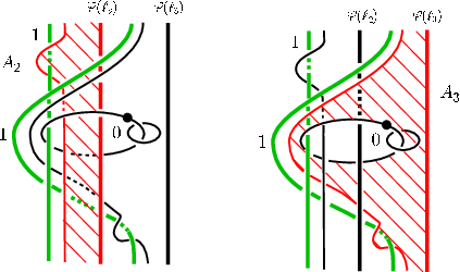
Hence $\pm 1$-fold Dehn twist along $T_{2}$ parallel to $K_{2}$ gives rise to the same manifolds $A_{K_{1}}$ and $\overline{C}\cup C_{K_{3},n}$. The integer $n$ is one of $\mp 1$, $\mp 9$. Here $K_{3}$ is the knot obtained by the $\pm 1$-Dehn surgery along $K_{2}$ as in Figure 8. By one strand twist in Section 2.2 we have $A_{K_{3}}\cong\overline{C}\cup C_{K_{3},n}\cong A_{K_{1}}$.

If we replace three strand twist with odd strand twist, we can construct diffeomorphisms.

Y. Ohyama in [Oh] has proven that local three strand twist is an unkotting operation of knots. Therefore for any knot $K$ there exists a finite sequence of local three strand twists: $K=k_{0}\to k_{1}\to\cdots\to k_{n}=\text{unknot}$. The sequence implies the sequence of diffeomorphisms:

$\Box$

Using the diffeomorphism, we obtain infinitely many embeddings:

However whether the embeddings are mutually non-diffeomorphic is unknown.

In this subsection we consider Scharlemann’s manifolds by the meridian $\gamma_{0}$. We remark the following.

In the case of $\epsilon=1$, we note the relationship between $B_{K}^{1}(\gamma_{0})$ and the knot surgery of the fishtail neighborhood.

The gluing map $\varphi_{0}$ satisfies (2) and $\varphi_{0}(\text{meridian of $K$})=$ the vanishing cycle. The resulting manifold

is Figure 20, where the picture is the case of $K=4_{1}$.

The manifolds obtained by the same meridian surgery on $S^{3}_{p}(K)\times S^{1}$ are diffeomorphic to $B_{K}^{\epsilon}(\gamma_{0})$ by one strand twist.

The fundamental group of $S^{3}_{-1}(3_{1})$ is

The set of free homotopy classes of maps $S^{1}\to S^{3}_{-1}(3_{1})$ is

and it possesses 9 classes as follows.

Each of the classes is a normal generator of the fundamental group except $[e],[x^{5}]$. Let $K$ be a knot in $S^{3}$. For $z\in\pi_{1}(S^{3}_{-1}(3_{1}))$ we define $B_{3_{1}}^{\epsilon}(z)$ to be the surgery of $S^{3}_{-1}(3_{1})\times S^{1}$ along a knot $K\subset S^{3}_{-1}(3_{1})$ whose free homotopy class $[K]$ coincides with the conjugacy class $[z]$. Akbulut’s result [Ak1] is that $B_{3_{1}}^{1}(x)$ is the standard $S^{2}\times S^{2}\#S^{3}\times S^{1}$. For other conjugacy class we will prove the following.

The case of $B_{3_{1}}^{0}(xy)$ is diffeomorphic to $S^{3}\times S^{1}\#{\mathbb{C}}P^{2}\#\overline{{\mathbb{C}}P^{2}}$ in the same way. $\Box$

Here we will argue several other cases.

Proof. Here we use notation $\approx$, $\sim$ and $=$ as one strand twist, a homeomorphism, Kirby calculus technique in 3-dimansional.

In the case of $B_{3_{1}}^{1}([x^{2}])$, the last picture in Figure 26 represents a surgery on $L(5,-1)\times S^{1}$. This is diffeomorphic to $S^{3}\times S^{1}\#{\mathbb{C}}P^{2}\#\overline{{\mathbb{C}}P^{2}}$.

In the case of $B_{3_{1}}^{0}([x^{3}])$ the last picture in Figure 27 represents a surgery along a knot $\gamma$ in $S^{3}\times S^{1}$ with odd framing. Namely the manifold is $S^{3}\times S^{1}\#{\mathbb{C}}P^{2}\#\overline{{\mathbb{C}}P^{2}}$.

In the case of $B_{3_{1}}^{1}([x^{4}])$, the last picture in Figure 28 gives $S^{3}\times S^{1}\#{\mathbb{C}}P^{2}\#\overline{{\mathbb{C}}P^{2}}$ in the similar way. Here $Pr(-2,3,7)$ is the $(-2,3,7)$-pretzel knot.

$\Box$

Proof. The homotopy cass of the curve $\gamma$ is $xyy^{-1}xy\sim x^{2}y\sim xyx$. then from the Figure 29, we get $S^{3}\times S^{1}\#{\mathbb{C}}P^{2}\#\overline{{\mathbb{C}}P^{2}}$. $\Box$.

Proof. The deformation as in Figure 30 we get $S^{3}\times S^{1}\#{\mathbb{C}}P^{2}\#\overline{{\mathbb{C}}P^{2}}$. Here $T_{2,7}$ is the $(2,7)$-torus knot $\Box$.

In the end we raise the questions.

References

- [Aka] M.Akaho, private communication, 2002
- [Ak1] S.Akbulut, Scharlemann’s manifold is standard, Annals of Mathematics, II. Series Vol. 149, No. 2, pp. 497-510 (1999)
- [Ak2] S.Akbulut, A fake cusp and a fishtail, Turkish Journal of Math. 23 (1999), no1, 19-31
- [Ak3] S.Akbulut, Twisting 4-manifolds along , arXiv:0912.4727v2
- [Ak4] S.Akbulut, Knot surgery and Scharlemann manifolds, arXiv:1011.6274v1
- [FS] R. Fintushel and R. Stern, Knot, links and 4-manifolds, Invent. Math. 134, no.2 (1998) 363-400.
- [GS] R. Gompf and Stipsicz, 4-manifolds and Kirby calculus, Graduate Studies in Mathematics, 20. American Mathematical Society, Providence, RI, 1999
- [G] R. Gompf, More Cappell-Shaneson spheres are standard, Algebraic & Geometry Topology 10(2010) 1665-1681
- [M] Y. Matsumoto, On 4-manifolds fibered by tori, Proc. Japan Acad. 58(1982), 298-301
- [Na] Y. Nakanishi, Replacements in the Conway third identity, Tokyo J. Math. 14 (1991), no. 1, 197–203.
- [Oh] Y. Ohyama, Twisting and unknotting operations, Rev. Mat. Univ. Complut. Madrid 7 (1994), no. 2, 289-305,
- [Sc] M. Scharlemann, Constructing strange manifolds with the dodecahedral space, Duke Math. J. 43 (1976) 33-40.
Research Institute for Mathematical Sciences, Kyoto University
Kitashirakawa Oiwake Sakyo-ku Kyoto-shi 606-8502
E-mail address: tange@kurims.kyoto-u.ac.jp