跳到论文正文
W Papers独立论文阅读器 arXiv:1011.5287 论文正文 计算阅读时间 · 0%
引用这篇论文根据当前论文元数据生成,正式投稿前建议核对。


License: arXiv.org perpetual non-exclusive license
arXiv:1011.5287v3 [cs.IT] 13 Jun 2012

Distributed Storage Allocations

Derek Leong, Alexandros G. Dimakis, and Tracey Ho ††thanks:  This paper is an extended version of [1], which is available online at http://dx.doi.org/10.1109/TIT.2012.2191135. The material in this paper was presented in part at the NetCod 2009 [2], ICC 2010 [3], and GLOBECOM 2010 [4] conferences.††thanks: The work of D.˜Leong and T.˜Ho was supported in part by Subcontract 069153 issued by BAE Systems National Security Solutions, Inc.˜and supported by the Defense Advanced Research Projects Agency (DARPA) and the Space and Naval Warfare System Center (SPAWARSYSCEN), San Diego, under Contract N66001-08-C-2013, by the Air Force Office of Scientific Research under Grant FA9550-10-1-0166, and by the Lee Center for Advanced Networking at the California Institute of Technology (Caltech). The work of D.˜Leong was supported in part by A*STAR, Singapore. The work of A.˜G.˜Dimakis was supported in part by the Center for the Mathematics of Information at Caltech, and by the National Science Foundation under NSF Grant 1055099.††thanks: D.˜Leong and T.˜Ho are with the Department of Electrical Engineering, California Institute of Technology, Pasadena, California 91125, USA (email: derekleong@caltech.edu, tho@caltech.edu).††thanks: A.˜G.˜Dimakis is with the Department of Electrical Engineering, University of Southern California, Los Angeles, California 90089, USA (email: dimakis@usc.edu).
Abstract

We examine the problem of allocating a given total storage budget in a distributed storage system for maximum reliability. A source has a single data object that is to be coded and stored over a set of storage nodes; it is allowed to store any amount of coded data in each node, as long as the total amount of storage used does not exceed the given budget. A data collector subsequently attempts to recover the original data object by accessing only the data stored in a random subset of the nodes. By using an appropriate code, successful recovery can be achieved whenever the total amount of data accessed is at least the size of the original data object. The goal is to find an optimal storage allocation that maximizes the probability of successful recovery. This optimization problem is challenging in general because of its combinatorial nature, despite its simple formulation. We study several variations of the problem, assuming different allocation models and access models. The optimal allocation and the optimal symmetric allocation (in which all nonempty nodes store the same amount of data) are determined for a variety of cases. Our results indicate that the optimal allocations often have nonintuitive structure and are difficult to specify. We also show that depending on the circumstances, coding may or may not be beneficial for reliable storage.

Index Terms: 
Data storage systems, distributed storage, network coding, reliability, storage allocation.

I Introduction

Consider a distributed storage system comprising nn storage nodes. A source has a single data object of normalized unit size that is to be coded and stored in a distributed manner over these nodes, subject to a given total storage budget TT. Let xix_{i} be the amount of coded data stored in node i∈i\in {1,…,n}\left\{1,\ldots,n\right\}. Any amount of data may be stored in each node, as long as the total amount of storage used over all nodes is at most the given budget TT, i.e.,

∑i=1nxi≤T.\sum_{i=1}^{n}x_{i}\leq T.

This is a realistic constraint if there is limited transmission bandwidth or storage space, or if it is too costly to mirror the data object in its entirety in every node. At some time after the creation of this coded storage, a data collector attempts to recover the original data object by accessing only the data stored in a random subset 𝐫{\mathbf{r}} of the nodes, where the probability distribution of 𝐫⊆{1,…,n}{\mathbf{r}}\subseteq{{\mbox{$\left\{1,\ldots,n\right\}$}}} is specified by an assumed access model or failure model (nodes or links may fail probabilistically, for example).
Refer to caption
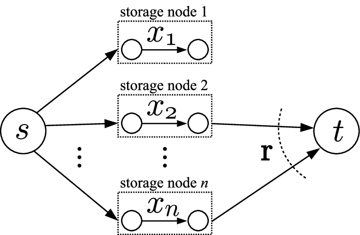
Fig. 1: Information flows in a distributed storage system. The source ss has a single data object of normalized unit size that is to be coded and stored over nn storage nodes. Subsequently, a data collector tt attempts to recover the original data object by accessing only the data stored in a random subset 𝐫{\mathbf{r}} of the nodes.

Fig. 1 depicts such a distributed storage system.

The reliability of this system, which we define to be the probability of successful recovery (or recovery probability in short), depends on both the storage allocation and the coding scheme. For maximum reliability, we would therefore need to find

  1. (i)

    an optimal allocation of the given budget TT over the nodes, specified by the values of x1,…,xnx_{1},\ldots,x_{n}, and

  2. (ii)

    an optimal coding scheme

that jointly maximize the probability of successful recovery. It turns out that these two problems can be decoupled by using a good coding scheme, specifically one that enables successful recovery whenever the total amount of data accessed by the data collector is at least the size of the original data object. This can be seen by considering the information flows for a network in which the source is multicasting the data object to a set of potential data collectors [5, 6]: successful recovery can be achieved by a data collector if and only if its corresponding max-flow or min-cut from the source is at least the size of the original data object. Random linear coding over a sufficiently large field would allow successful recovery with high probability when this condition is satisfied [7, 8]. Alternatively, a suitable maximum distance separable (MDS) code for the given budget and data object size would allow successful recovery with certainty when this condition is satisfied.

Therefore, assuming the use of an appropriate code, the probability of successful recovery for an allocation (x1,…,xn)\left(x_{1},\ldots,x_{n}\right) can be written as

ℙ[successful recovery]=ℙ[∑i∈𝐫xi≥1].{\mathbb{P}\left[\text{successful recovery}\right]}={\mathbb{P}\left[\sum_{i\in{\mathbf{r}}}x_{i}\geq 1\right]}.

Our goal is to find an optimal allocation that maximizes this recovery probability, subject to the given budget constraint.

Although we have assumed coded storage at the outset, coding may ultimately be unnecessary for certain allocations. For example, if the budget is spread minimally such that each nonempty node stores the data object in its entirety (i.e., xi≥1x_{i}\geq 1 for all i∈Si\in S, and xi=0x_{i}=0 for all i∉Si\notin S, where SS is some subset of {1,…,n}\left\{1,\ldots,n\right\}), then uncoded replication would suffice since the data object can be recovered by accessing any one nonempty node; the data collector would not need to combine data accessed from different nodes in order to recover the data object. Thus, by solving for the optimal allocation, we will also be able to determine whether coding is beneficial for reliable storage.

We note that even though no explicit upper bound is imposed on the amount of data that can be stored in each node, it is never necessary to set xi>1x_{i}>1 because xi=1x_{i}=1 already allows the data object to be stored in its entirety in that node. The absence of a tighter per-node storage constraint xi≤ci<1x_{i}\leq c_{i}<1 is reasonable for storage systems that handle a large number of data objects: we would expect the storage capacity of each node to be much larger than the size of a single data object, making it possible for a node to accommodate some of the data objects in their entirety. As such, it would be appropriate to apply a storage constraint for each data object via the budget TT, without a separate a priori constraint for xix_{i}. Furthermore, the simplifying assumption of xix_{i} being a continuous variable is a reasonable one for large data objects: a large data object size would facilitate the creation of coded data packets with sizes (closely) matching that of a desired allocation. Incidentally, the overhead associated with random linear coding or an MDS code, which is ignored in our model, becomes proportionately negligible when the amount of coded data is large.

In spite of the simple formulation, this optimization problem poses significant challenges because of its combinatorial nature and the large space of feasible allocations. Different variations of this problem can be formulated by assuming different allocation models and access models; in this paper, we will examine three such variations that are motivated by practical storage problems in content delivery networks, delay tolerant networks, and wireless sensor networks.

I-A Independent Probabilistic Access to Each Node

In the first problem formulation, we assume that the data collector accesses each of the nn nodes independently with constant probability pp; in other words, each node ii appears in subset 𝐫{\mathbf{r}} independently with probability pp. The resulting problem can be interpreted as that of maximizing the reliability of data storage in a system comprising nn storage devices where each device fails independently with probability 1−p1-p. It is not hard to show that determining the recovery probability of a given allocation is computationally difficult (specifically, #P-hard). The intuitive approach of spreading the budget maximally over all nodes, i.e., setting xi=Tnx_{i}=\frac{T}{n} for all ii, turns out to be not necessarily optimal; in fact, the optimal allocation may not even be symmetric (we say that an allocation is symmetric when all nonzero xix_{i} are equal). The following counterexample from [9] demonstrates that symmetric allocations can be suboptimal: for (n,p,T)(n,p,T) == (5,23,73)\left(5,\frac{2}{3},\frac{7}{3}\right), the nonsymmetric allocation

(23,23,13,13,13),\textstyle\left(\frac{2}{3},\frac{2}{3},\frac{1}{3},\frac{1}{3},\frac{1}{3}\right),

which achieves a recovery probability of 0.905350.90535, performs strictly better than any symmetric allocation; the maximum recovery probability among symmetric allocations is 0.888890.88889, which is achieved by both

(76,76,0,0,0)​ and ​(712,712,712,712,0).\textstyle\left(\frac{7}{6},\frac{7}{6},0,0,0\right)\text{ and }\left(\frac{7}{12},\frac{7}{12},\frac{7}{12},\frac{7}{12},0\right).

Evidently, the simple strategy of “spreading eggs evenly over more baskets” may not always improve the reliability of an allocation.

Our Contribution: We show that the intuitive symmetric allocation that spreads the budget maximally over all nodes is indeed asymptotically optimal in a regime of interest. Specifically, we derive an upper bound for the suboptimality of this allocation, and show that the performance gap vanishes asymptotically as the total number of storage nodes nn grows, when p>1Tp>\frac{1}{T}. This is a regime of interest because a high recovery probability is possible when p>1Tp>\frac{1}{T} ⟺\Longleftrightarrow p​T>1pT>1: The expected total amount of data accessed by the data collector is given by

𝔼⁡[∑i=1nxi​Yi]=∑i=1nxi​𝔼​[Yi]=p​∑i=1nxi≤p​T,\displaystyle{\mathbb{E}\left[\displaystyle\sum_{i=1}^{n}x_{i}Y_{i}\right]}=\sum_{i=1}^{n}x_{i}{\mathbb{E}\left[Y_{i}\right]}=p\sum_{i=1}^{n}x_{i}\leq pT, (1)

where YiY_{i}’s are independent Bernoulli​(p)\text{Bernoulli}(p) random variables. Therefore, the data collector would be able to access a sufficient amount of data in expectation for successful recovery if p​T>1pT>1.

We also show that the symmetric allocation that spreads the budget minimally is optimal when pp is sufficiently small. In such an allocation, the data object is stored in its entirety in each nonempty node, making coding unnecessary. Additionally, we explicitly find the optimal symmetric allocation for a wide range of parameter values of pp and TT.

Related Work: This problem was introduced to us through a discussion at UC Berkeley [9]. We have since learned that variations of the problem have also been studied in several different fields.

In reliability engineering, the weighted-kk-out-of-nn system [10] comprises nn components, each having a positive integer weight wiw_{i} and surviving independently with probability pip_{i}; the system is in a good state if and only if the total weight of its surviving components is at least a specified threshold kk. Related work on this system and its extensions has focused on the efficient computation of the reliability of a given weight allocation (see, e.g., [11]).

In peer-to-peer networking, the allocation problem deals with the recovery of a data object from peers that are available only probabilistically. Lin et al. [12] compared the performance of uncoded replication vs. coded storage, restricted to symmetric allocations, for the case where the budget is an integer.

In wireless communications, the allocation problem is studied in the context of multipath routing, in which coded data is transmitted along different paths in an unreliable network, exploiting path diversity to improve the reliability of end-to-end communications. Tsirigos and Haas [13, 14] examined the performance of symmetric allocations and noted the existence of a phase transition in the optimal symmetric allocation; approximation methods were also proposed by the authors to tackle the optimization problem, especially for the case where path failures occur with nonuniform probabilities and may be correlated. Jain et al. [15] evaluated the performance of symmetric allocations experimentally in a delay tolerant network setting, and presented an alternative formulation using Gaussian distributions to model partial access to nodes.

Our work generalizes these previous efforts by considering nonsymmetric allocations and noninteger budgets. We also correct some inaccurate claims about the optimal symmetric allocation in [15] and its associated technical report.

I-B Access to a Random Fixed-Size Subset of Nodes

In the second problem formulation, we assume that the data collector accesses an rr-subset of the nn nodes selected uniformly at random from the collection of all (nr)\left(\genfrac{}{}{0.0pt}{}{n}{r}\right) possible rr-subsets, where rr is a given constant. The resulting problem can be interpreted as that of maximizing the recovery probability in a networked storage system of nn nodes where the end user is able or allowed to contact up to rr nodes randomly. We can treat this access model as an approximation to the preceding independent probabilistic access model by picking r≈n​pr\approx np. Finding the optimal allocation in this case is still challenging. As in the first problem formulation, it is not hard to show that determining the recovery probability of a given allocation is computationally difficult (specifically, #P-complete).

The problem appears nontrivial even if we restrict the optimization to only symmetric allocations. Numerically, we observe that given nn and rr, either a minimal or a maximal spreading of the budget is optimal among symmetric allocations for most, if not all, choices of TT. One example of an exception is (n,r,T)(n,r,T) == (14,5,83)\left(14,5,\frac{8}{3}\right) for which it is optimal to have 88 nonempty nodes in the symmetric allocation, instead of the extremes 22 or 1313; another example is (n,r,T)(n,r,T) == (16,4,72)\left(16,4,\frac{7}{2}\right) for which it is optimal to have 77 nonempty nodes in the symmetric allocation, instead of the extremes 33 or 1414. Furthermore, the number of nonempty nodes in the optimal symmetric allocation is not necessarily a nondecreasing function of the budget TT; for instance, given (n,r)(n,r) == (20,4)(20,4), it is optimal to have (4,18,14,19,20)(4,18,14,19,20) nonempty nodes in the symmetric allocation for T=(4.25,4.5,4.67,4.75,5)T=(4.25,4.5,4.67,4.75,5), respectively.

Our Contribution: We show that the allocation (1r,…,1r)\left(\frac{1}{r},\ldots,\frac{1}{r}\right) is optimal in the high recovery probability regime. Specifically, we demonstrate that this allocation, which has a recovery probability of exactly 11, minimizes the budget TT necessary for achieving any recovery probability exceeding a specified threshold 1−ϵ1-\epsilon. Although ϵ\epsilon depends on nn and rr in a complicated way, we can conclude that for any rr, this allocation is optimal if the recovery probability is to exceed 1−1n1-\frac{1}{n}.

We also make the following conjecture about the optimal allocation, based on our numerical observations:

Conjecture.

A symmetric optimal allocation always exists for any nn, rr, and TT.

Related Work: Sardari et al. [16] presented a method of approximating an optimal solution to this problem by considering a data collector that accesses rr random nodes with replacement. More recently, Alon et al. [17] showed that this problem is related to an old conjecture by Erdős on the maximum number of edges in a uniform hypergraph [18].

I-C Probabilistic Symmetric Allocations

In the third problem formulation, we assume a probabilistic allocation model in which the source selects a random allocation from a distribution of allocations, with the constraint that the expected total amount of storage used in an allocation is at most the given budget TT. We specifically consider the case where each of the nn nodes is selected by the source independently with constant probability min⁡(ℓ​Tn,1)\min\!\left(\frac{\ell T}{n},1\right) to store a constant 1ℓ\frac{1}{\ell} amount of data, thus creating a probabilistic symmetric allocation of the budget. The data collector subsequently accesses an rr-subset of the nn nodes selected uniformly at random from the collection of all (nr)\left(\genfrac{}{}{0.0pt}{}{n}{r}\right) possible rr-subsets, where rr is a given constant. The goal is to find an optimal allocation, specified by the value of parameter ℓ\ell, that maximizes the recovery probability. This model was conceived as a simplification of the preceding fixed-size subset access model which assumes a deterministic allocation of the budget.

Our Contribution: We show that the choice of ℓ=r\ell=r, which corresponds to a maximal spreading of the budget, is optimal when the given budget TT is sufficiently large, or equivalently, when a sufficiently high recovery probability (specifically, 34\frac{3}{4} or higher) is achievable. We believe this is a reasonable operating regime for applications that require good reliability.

I-D Other Related Work

Apart from the work done on the preceding problems, a variety of storage allocation problems have also been studied in a nonprobabilistic setting. For instance, the objective adopted in [19] and [20] is to minimize the total storage budget required to satisfy a given set of deterministic recovery requirements in a network. Incidentally, the use of network coding makes it easier to deal with the total cost of content delivery, which covers the initial dissemination, storage, and eventual fetching of data objects; this cost-minimization problem is considered in [6] and [21], subject to various deterministic constraints involving, for example, load balancing or fetching distance.

We note that in most of the literature involving reliable distributed storage, either the data object is assumed to be replicated in its entirety (see, e.g., [22]), or, if coding is used, every node is assumed to store the same amount of coded data (see, e.g., [23, 24, 25, 26, 27]). Allocations of a storage budget with nodes possibly storing different amounts of data are not usually considered.

In the following three sections, we define each problem formally and state our main results. Proofs of theorems are deferred to the appendix. Table I summarizes the notation used throughout this paper.

TABLE I: Notation
Symbol Definition
nn total number of storage nodes, n≥2n\geq 2
xix_{i} amount of data stored in storage node ii,
xi≥0x_{i}\geq 0, where i∈i\in {1,…,n}\left\{1,\ldots,n\right\}
TT total storage budget, 1≤T≤n1\leq T\leq n
𝐫{\mathbf{r}} subset of nodes accessed, 𝐫⊆{\mathbf{r}}\subseteq {1,…,n}\left\{1,\ldots,n\right\}
pp access probability (Section II), 0<p<10<p<1
rr number of nodes accessed (Section III), 1≤r≤n1\leq r\leq n
1ℓ\frac{1}{\ell} amount of data stored in each nonempty node
(Section IV), ℓ>0\ell>0
ℬ⁡(n,p){\mathcal{B}\left(n,p\right)} binomial random variable with nn trials and
success probability pp
1​[G]{\mathbbold{1}\left[G\right]} indicator function; 1​[G]=1{\mathbbold{1}\left[G\right]}=1 if statement GG is true,
and 00 otherwise
ℤ0+{\mathbb{Z}}^{+}_{0} the set of nonnegative integers, i.e., ℤ+∪{0}{\mathbb{Z}}^{+}\cup\{0\}

II Independent Probabilistic Access to Each Node

In the first variation of the storage allocation problem, we consider a data collector that accesses each of the nn nodes independently with probability pp; successful recovery occurs if and only if the total amount of data stored in the accessed nodes is at least 11. We seek an optimal allocation (x1,…,xn)\left(x_{1},\ldots,x_{n}\right) of the budget TT that maximizes the probability of successful recovery, for a given choice of nn, pp, and TT. This optimization problem can be expressed as follows:

𝚷1​(n,p,T):\displaystyle\hskip-3.00003pt{\mathbf{\Pi}}_{1}(n,p,T):
maximizex1,…,xn∑𝐫⊆{1,…,n}p|𝐫|(1−p)n−|𝐫|⋅1[∑i∈𝐫xi≥1]\displaystyle\hskip 3.99994pt\underset{x_{1},\ldots,x_{n}}{\text{maximize}}\sum_{{\mathbf{r}}\subseteq\{1,\ldots,n\}}p^{|{\mathbf{r}}|}(1-p)^{n-|{\mathbf{r}}|}\cdot{\mathbbold{1}\left[\sum_{i\in{\mathbf{r}}}x_{i}\geq 1\right]} (2)
 subject to
∑i=1nxi≤T\displaystyle\hskip 46.5pt\sum_{i=1}^{n}x_{i}\hskip 0.0pt\leq\hskip 5.0ptT (3)
xi≥0∀i∈{1,…,n}.\displaystyle\hskip 59.00002ptx_{i}\hskip 5.0pt\geq\hskip 5.0pt0\hskip 20.50006pt\forall\;\;i\in{{\mbox{$\left\{1,\ldots,n\right\}$}}}. (4)

The objective function (2) is just the recovery probability, expressed as the sum of the probabilities corresponding to the subsets 𝐫{\mathbf{r}} that allow successful recovery. An equivalent expression for (2) is

ℙ[∑i=1nxiYi≥1],{\mathbb{P}\left[\sum_{i=1}^{n}x_{i}\,Y_{i}\geq 1\right]},

where YiY_{i}’s are independent Bernoulli​(p)\text{Bernoulli}(p) random variables. Inequality (3) expresses the budget constraint, and inequality (4) ensures that a nonnegative amount of data is stored in each node. For the trivial budget T=1T=1, the allocation (1,0,…,0)(1,0,\ldots,0) is optimal; for T=nT=n, the allocation (1,…,1)(1,\ldots,1) is optimal. Incidentally, computing the recovery probability of a given allocation turns out to be #P-hard:

Proposition 1.

Computing the recovery probability

∑𝐫⊆{1,…,n}p|𝐫|(1−p)n−|𝐫|⋅1[∑i∈𝐫xi≥1]\sum_{{\mathbf{r}}\subseteq\{1,\ldots,n\}}p^{|{\mathbf{r}}|}(1-p)^{n-|{\mathbf{r}}|}\cdot{\mathbbold{1}\left[\sum_{i\in{\mathbf{r}}}x_{i}\geq 1\right]}

for a given allocation (x1,…,xn)\left(x_{1},\ldots,x_{n}\right) and choice of pp is #P-hard.

TABLE II: Optimal Allocations for Number of Nodes n=2,3,4n=2,3,4
nn Budget TT Optimalallocation\begin{array}[]{l}\text{Optimal}\\ \text{allocation}\end{array} Condition on access probability p(if any)\begin{array}[]{l}\text{Condition on access probability $p$}\\ \text{(if any)}\end{array}
22 1≤T<21\leq T<2 (1,0)\left(1,0\right)
33 1≤T<321\leq T<\frac{3}{2} (1,0,0)\left(1,0,0\right)
32≤T<2\frac{3}{2}\leq T<2 (1,0,0)\left(1,0,0\right) if p≤12p\leq\frac{1}{2}
(12,12,12)\left(\frac{1}{2},\frac{1}{2},\frac{1}{2}\right) if p≥12p\geq\frac{1}{2}
2≤T<32\leq T<3 (1,1,0)\left(1,1,0\right)
44 1≤T<431\leq T<\frac{4}{3} (1,0,0,0)\left(1,0,0,0\right)
43≤T<32\frac{4}{3}\leq T<\frac{3}{2} (1,0,0,0)\left(1,0,0,0\right) if p≤1+136≈0.768p\leq\frac{1+\sqrt{13}}{6}\approx 0.768
(13,13,13,13)\left(\frac{1}{3},\frac{1}{3},\frac{1}{3},\frac{1}{3}\right) if p≥1+136≈0.768p\geq\frac{1+\sqrt{13}}{6}\approx 0.768
32≤T<2\frac{3}{2}\leq T<2 (1,0,0,0)\left(1,0,0,0\right) if p≤12p\leq\frac{1}{2}
(12,12,12,0)\left(\frac{1}{2},\frac{1}{2},\frac{1}{2},0\right) if p≥12p\geq\frac{1}{2}
2≤T<522\leq T<\frac{5}{2} (1,1,0,0)\left(1,1,0,0\right) if p≤23p\leq\frac{2}{3}
(12,12,12,12)\left(\frac{1}{2},\frac{1}{2},\frac{1}{2},\frac{1}{2}\right) if p≥23p\geq\frac{2}{3}
52≤T<3\frac{5}{2}\leq T<3 (1,1,0,0)\left(1,1,0,0\right) if p≤12p\leq\frac{1}{2}
(1,12,12,12)\left(1,\frac{1}{2},\frac{1}{2},\frac{1}{2}\right) if p≥12p\geq\frac{1}{2}
3≤T<43\leq T<4 (1,1,1,0)\left(1,1,1,0\right)

Table II lists the optimal allocations for n=2,3,4n=2,3,4, covering all parameter values of p∈(0,1)p\in(0,1) and T∈[1,n)T\in[1,n). These solutions are obtained by minimizing TT for each possible value of the objective function (2). We observe that

  1. (i)

    for any TT, the symmetric allocation (1,…,1,0,…,0)(1,\ldots,1,0,\ldots,0), which corresponds to a minimal spreading of the budget (uncoded replication), appears to be optimal when pp is sufficiently small, and

  2. (ii)

    the optimal symmetric allocation appears to perform well despite being suboptimal in some cases, e.g., when (n,T)=(4,52)(n,T)=\left(4,\frac{5}{2}\right) and p>12p>\frac{1}{2}.

We will proceed to show that observation (i) is indeed true in Section II-B; the opposite approach of spreading the budget maximally over all nodes turns out to be asymptotically optimal when pp is sufficiently large, as will be demonstrated in Section II-A. Motivated by observation (ii), we examine the optimization problem restricted to symmetric allocations in Section II-C.

For brevity, let 𝐱¯​(n,T,m){\bar{\mathbf{x}}}(n,T,m) denote the symmetric allocation for nn nodes that uses a total storage of TT and contains exactly m∈{1,2,…,n}m\in\{1,2,\ldots,n\} nonempty nodes:

𝐱¯​(n,T,m)≜(Tm,…,Tm⏟m​ entries,0,…,0⏟(n−m)​ entries).{\bar{\mathbf{x}}}(n,T,m)\triangleq\biggl(\,\underbrace{\frac{T}{m},\ldots,\frac{T}{m}}_{m\text{ entries}},\underbrace{0,\ldots,0\vphantom{\frac{T}{m}}}_{(n-m)\text{ entries}}\!\!\biggr).

Since successful recovery for the symmetric allocation 𝐱¯​(n,T,m){\bar{\mathbf{x}}}(n,T,m) occurs if and only if at least ⌈1/(Tm)⌉{\left\lceil{1\big/\left(\frac{T}{m}\right)}\right\rceil} =⌈mT⌉={\left\lceil{\frac{m}{T}}\right\rceil} out of the mm nonempty nodes are accessed, the corresponding probability of successful recovery can be written as

PS(p,T,m)≜ℙ[ℬ(m,p)≥⌈mT⌉].{P_{\text{S}}}(p,T,m)\triangleq{\mathbb{P}\left[\displaystyle{\mathcal{B}\left(m,p\right)}\geq{\left\lceil{\frac{m}{T}}\right\rceil}\right]}.

II-A Asymptotic Optimality of Maximal Spreading

The recovery probability of the symmetric allocation 𝐱¯​(n,T,m=n){\bar{\mathbf{x}}}\left(n,T,m{=}n\right), which corresponds to a maximal spreading of the budget over all nodes, is given by

PS(p,T,m=n)=ℙ[ℬ(n,p)≥⌈nT⌉].\displaystyle{P_{\text{S}}}(p,T,m{=}n)={\mathbb{P}\left[\displaystyle{\mathcal{B}\left(n,p\right)}\geq{\left\lceil{\frac{n}{T}}\right\rceil}\right]}. (5)

To establish the optimality of this allocation, we compare (5) to an upper bound for the recovery probability of an optimal allocation. Such a bound can be derived by conditioning on the number of accessed nodes:

Lemma 1.

The probability of successful recovery for an optimal allocation is at most

∑r=0nmin(r​Tn,1)ℙ[ℬ(n,p)=r].\displaystyle\sum_{r=0}^{n}\min\left(\frac{rT}{n},1\right)\;{\mathbb{P}\left[{\mathcal{B}\left(n,p\right)}=r\right]}. (6)

The suboptimality of 𝐱¯​(n,T,m=n){\bar{\mathbf{x}}}\left(n,T,m{=}n\right) is therefore bounded by the difference between (5) and (6), as given by the following theorem; when p>1Tp>\frac{1}{T}, this allocation becomes asymptotically optimal since its suboptimality gap vanishes as nn goes to infinity:

Theorem 1.

The gap between the probabilities of successful recovery for an optimal allocation and for the symmetric allocation 𝐱¯​(n,T,m=n){\bar{\mathbf{x}}}\left(n,T,m{=}n\right), which corresponds to a maximal spreading of the budget over all nodes, is at most

pTℙ[ℬ(n−1,p)≤⌈nT⌉−2].p\,T\;{\mathbb{P}\left[\displaystyle{\mathcal{B}\left(n-1,p\right)}\leq{\left\lceil{\frac{n}{T}}\right\rceil}-2\right]}.

If pp and TT are fixed such that p>1Tp>\frac{1}{T}, then this gap approaches zero as nn goes to infinity.

We note that the regime p>1Tp>\frac{1}{T} is particularly interesting because it corresponds to the regime of high recovery probability; the recovery probability would be bounded away from 11 if p<1Tp<\frac{1}{T} ⟺\Longleftrightarrow p​T<1pT<1 instead. This follows from the application of Markov’s inequality to the random variable WW denoting the total amount of data accessed by the data collector, which produces

ℙ[W≥1]≤𝔼[W].{\mathbb{P}\left[W\geq 1\right]}\leq{\mathbb{E}\left[W\right]}.

Since ℙ[W≥1]{\mathbb{P}\left[W\geq 1\right]} is just the probability of successful recovery, and 𝔼⁡[W]≤p​T{\mathbb{E}\left[W\right]}\leq pT according to (1), we have

ℙ⁡[successful recovery]≤p​T.{\mathbb{P}\left[\text{successful recovery}\right]}\leq pT.

II-B Optimality of Minimal Spreading (Uncoded Replication)

The recovery probability of the symmetric allocation 𝐱¯​(n,T,m=⌊T⌋){\bar{\mathbf{x}}}\left(n,T,m{=}{\left\lfloor{T}\right\rfloor}\right), which corresponds to a minimal spreading of the budget, is given by

PS(p,T,m=⌊T⌋)=ℙ[ℬ(⌊T⌋,p)≥1]=1−(1−p)⌊T⌋.\displaystyle{P_{\text{S}}}\left(p,T,m{=}{\left\lfloor{T}\right\rfloor}\right)={\mathbb{P}\left[\displaystyle{\mathcal{B}\left({\left\lfloor{T}\right\rfloor},p\right)}{\geq}1\right]}=1-(1{-}p)^{{\left\lfloor{T}\right\rfloor}}. (7)

Recall that coding is unnecessary in such an allocation since the data object is stored in its entirety in each nonempty node. A sufficient condition for the optimality of this allocation can be found by comparing (7) to an upper bound for the recovery probabilities of all other allocations. Our approach is to classify each allocation according to the number of individual nodes that store at least a unit amount of data. We then find a bound for allocations containing exactly 00 such nodes, another bound for allocations containing exactly 11 such node, and so on. The subsequent comparisons of (7) to each of these bounds result in the following theorem:

Theorem 2.

If 1<T<n1<T<n and

1−(1−p)⌊T⌋−n+(n−ℓ)​(p1−p)\displaystyle 1-(1-p)^{{\left\lfloor{T}\right\rfloor}-n}+(n-\ell)\left(\frac{p}{1-p}\right)
+∑r=2⌈n−ℓT−ℓ⌉−1(1−T−ℓn−ℓ⋅r)(n−ℓr)(p1−p)r≥0\displaystyle\;\;+\!\!\sum_{r=2}^{{\left\lceil{\frac{n-\ell}{T-\ell}}\right\rceil}-1}\left(1-\frac{T-\ell}{n-\ell}\cdot r\right)\left(\genfrac{}{}{0.0pt}{}{n-\ell}{r}\right)\left(\frac{p}{1-p}\right)^{r}\geq 0 (8)

for all ℓ∈{0,1,…,⌊T⌋−1}\ell\in\{0,1,\ldots,{\left\lfloor{T}\right\rfloor}-1\}, then 𝐱¯​(n,T,m=⌊T⌋){\bar{\mathbf{x}}}\left(n,T,m{=}{\left\lfloor{T}\right\rfloor}\right), which corresponds to a minimal spreading of the budget (uncoded replication), is an optimal allocation.

The following corollary shows that this allocation is indeed optimal for sufficiently small pp:

Corollary 1.

If 1<T<n1<T<n and p≤2(n−⌊T⌋)2p\leq\frac{2}{\left(n-{\left\lfloor{T}\right\rfloor}\right)^{2}}, then 𝐱¯​(n,T,m=⌊T⌋){\bar{\mathbf{x}}}\left(n,T,m{=}{\left\lfloor{T}\right\rfloor}\right) is an optimal allocation.

Refer to caption
Fig. 2: Plot of access probability pp against budget TT, showing regions of (T,p)(T,p) over which the sufficient conditions of the theorems are satisfied, for n=20n=20. Minimal spreading (uncoded replication) is optimal among all allocations in the colored regions.

Fig. 2 illustrates these results in the form of a region plot for an instance of nn.

II-C Optimal Symmetric Allocation

The optimization problem appears nontrivial even if we were to consider only symmetric allocations.

Refer to caption
Fig. 3: Plot of recovery probability PS{P_{\text{S}}} against budget TT for each symmetric allocation 𝐱¯​(n,T,m){\bar{\mathbf{x}}}(n,T,m), for (n,p)=(20,35)(n,p)=\left(20,\frac{3}{5}\right). Parameter mm denotes the number of nonempty nodes in the symmetric allocation. The black curve gives an upper bound for the recovery probability of an optimal allocation, as derived in Lemma 1.

Fig. 3, which compares the performance of different symmetric allocations over different budgets for an instance of (n,p)(n,p), demonstrates that the value of mm corresponding to the optimal symmetric allocation can change drastically as the budget TT varies.

Fortunately, we can eliminate many candidates for the optimal value of mm by making the following observation: Recall that the recovery probability of the symmetric allocation 𝐱¯​(n,T,m){\bar{\mathbf{x}}}(n,T,m) is given by PS​(p,T,m){P_{\text{S}}}(p,T,m) ≜\triangleq ℙ[ℬ(m,p)≥⌈mT⌉]{\mathbb{P}\left[{\mathcal{B}\left(m,p\right)}\geq{\left\lceil{\frac{m}{T}}\right\rceil}\right]}. For fixed nn, pp, and TT, we have

⌈mT⌉\displaystyle{\left\lceil{\frac{m}{T}}\right\rceil} =kwhen ​m∈((k−1)​T,k​T],\displaystyle=k\hskip 45.00006pt\text{when }m\in\big((k-1)T,kT\big],
for k=1,2,…,⌊nT⌋k=1,2,\ldots,{\left\lfloor{\frac{n}{T}}\right\rfloor}, and finally,
⌈mT⌉\displaystyle{\left\lceil{\frac{m}{T}}\right\rceil} =⌊nT⌋+1when ​m∈(⌊nT⌋​T,n].\displaystyle={\left\lfloor{\frac{n}{T}}\right\rfloor}+1\hskip 13.20009pt\text{when }m\in\left({\left\lfloor{\frac{n}{T}}\right\rfloor}T,n\right].

Since ℙ[ℬ(m,p)≥k]{\mathbb{P}\left[{\mathcal{B}\left(m,p\right)}\geq k\right]} is nondecreasing in mm for constant pp and kk, it follows that PS​(p,T,m){P_{\text{S}}}(p,T,m) is maximized within each of these intervals of mm when we pick mm to be the largest integer in the corresponding interval. Thus, given nn, pp, and TT, we can find an optimal m∗m^{*} that maximizes PS​(p,T,m){P_{\text{S}}}(p,T,m) over all mm from among ⌈nT⌉{\left\lceil{\frac{n}{T}}\right\rceil} candidates:

{⌊T⌋,⌊2​T⌋,…,⌊⌊nT⌋​T⌋,n}.\displaystyle\left\{{\left\lfloor{T}\right\rfloor},{\left\lfloor{2T}\right\rfloor},\ldots,{\left\lfloor{{\left\lfloor{\frac{n}{T}}\right\rfloor}T}\right\rfloor},n\right\}. (9)

For m=⌊k​T⌋m={\left\lfloor{kT}\right\rfloor}, where k∈ℤ+k\in{\mathbb{Z}}^{+}, the corresponding probability of successful recovery is given by

PS​(p,T,m=⌊k​T⌋)=ℙ[ℬ(⌊kT⌋,p)≥k].{{\mbox{${P_{\text{S}}}\left(p,T,m{=}{\left\lfloor{kT}\right\rfloor}\right)$}}}={\mathbb{P}\left[{\mathcal{B}\left({\left\lfloor{kT}\right\rfloor},p\right)}\geq k\right]}.

The difference between the probabilities of successful recovery for consecutive values of k∈ℤ+k\in{\mathbb{Z}}^{+} can be written as

Δ⁡(p,T,k)≜PS​(p,T,m=⌊(k+1)​T⌋)−PS​(p,T,m=⌊k​T⌋)\displaystyle\Delta(p,T,k)\triangleq{{\mbox{${P_{\text{S}}}\left(p,T,m{=}{\left\lfloor{(k+1)T}\right\rfloor}\right)$}}}-{{\mbox{${P_{\text{S}}}\left(p,T,m{=}{\left\lfloor{kT}\right\rfloor}\right)$}}}
=ℙ[ℬ(⌊(k+1)T⌋,p)≥k+1]−ℙ[ℬ(⌊kT⌋,p)≥k]\displaystyle\;\;={\mathbb{P}\left[{\mathcal{B}\left({\left\lfloor{(k+1)T}\right\rfloor},p\right)}\geq k+1\right]}-{\mathbb{P}\left[{\mathcal{B}\left({\left\lfloor{kT}\right\rfloor},p\right)}\geq k\right]}
=∑i=1min⁡(αk,T−1,k)ℙ[ℬ(⌊kT⌋,p)=k−i]⋅ℙ[ℬ(αk,T,p)≥i+1]\displaystyle\;\;=\hskip-20.00003pt\sum_{i=1}^{\min(\alpha_{k,T}-1,k)}\hskip-15.00002pt{\mathbb{P}\left[{\mathcal{B}\left({\left\lfloor{kT}\right\rfloor},p\right)}=k-i\right]}\cdot{\mathbb{P}\left[{\mathcal{B}\left(\alpha_{k,T},p\right)}\geq i+1\right]}
−ℙ[ℬ(⌊kT⌋,p)=k]⋅ℙ[ℬ(αk,T,p)=0],\displaystyle\;\;\hskip 11.99998pt-{\mathbb{P}\left[{\mathcal{B}\left({\left\lfloor{kT}\right\rfloor},p\right)}=k\right]}\cdot{\mathbb{P}\left[{\mathcal{B}\left(\alpha_{k,T},p\right)}=0\right]},

where αk,T≜⌊(k+1)​T⌋−⌊k​T⌋\alpha_{k,T}\triangleq{\left\lfloor{(k+1)T}\right\rfloor}-{\left\lfloor{kT}\right\rfloor}. The above expression is obtained by comparing the branches of the probability tree for ⌊k​T⌋{\left\lfloor{kT}\right\rfloor} vs. ⌊(k+1)​T⌋{\left\lfloor{(k+1)T}\right\rfloor} independent Bernoulli​(p)\text{Bernoulli}(p) trials: the first term describes unsuccessful events (“ℬ⁡(⌊k​T⌋,p)<k{\mathcal{B}\left({\left\lfloor{kT}\right\rfloor},p\right)}<k”) becoming successful (“ℬ⁡(⌊(k+1)​T⌋,p)≥k+1{\mathcal{B}\left({\left\lfloor{(k+1)T}\right\rfloor},p\right)}\geq k+1”) after the additional αk,T\alpha_{k,T} trials, while the second term describes successful events (“ℬ⁡(⌊k​T⌋,p)≥k{\mathcal{B}\left({\left\lfloor{kT}\right\rfloor},p\right)}\geq k”) becoming unsuccessful (“ℬ⁡(⌊(k+1)​T⌋,p)<k+1{\mathcal{B}\left({\left\lfloor{(k+1)T}\right\rfloor},p\right)}<k+1”) after the additional αk,T\alpha_{k,T} trials. After further simplification, we arrive at

Δ(p,T,k)=pk(1−p)⌊(k+1)​T⌋−k⋅\displaystyle\Delta(p,T,k)=p^{k}(1-p)^{{\left\lfloor{(k+1)T}\right\rfloor}-k}\cdot
{∑i=1min⁡(αk,T−1,k)∑j=i+1αk,T(⌊k​T⌋k−i)​(αk,Tj)​(p1−p)−i+j−(⌊k​T⌋k)}.\displaystyle{\scriptsize\begin{array}[]{l}\displaystyle\;\,\left\{\sum_{i=1}^{\min\big(\alpha_{k,T}-1,k\big)}\sum_{j=i+1}^{\alpha_{k,T}}\left(\genfrac{}{}{0.0pt}{}{\floor{kT}}{k-i}\right)\left(\genfrac{}{}{0.0pt}{}{\alpha_{k,T}}{j}\right)\left(\frac{p}{1-p}\right)^{-i+j}\!\!-\left(\genfrac{}{}{0.0pt}{}{\floor{kT}}{k}\right)\right\}\!.\end{array}}

The following theorem essentially provides a sufficient condition on pp and TT for Δ⁡(p,T,k)≥0\Delta(p,T,k)\geq 0 for any k∈ℤ+k\in{\mathbb{Z}}^{+}, thereby eliminating all but the two largest candidate values for m∗m^{*} in (9), i.e., m=⌊⌊nT⌋​T⌋m={\left\lfloor{{\left\lfloor{\frac{n}{T}}\right\rfloor}T}\right\rfloor} and m=nm=n, which correspond to a maximal spreading of the budget over (almost) all nodes (they are identical when nT∈ℤ+\frac{n}{T}\in{\mathbb{Z}}^{+}, i.e., T=n,n2,n3,…T=n,\frac{n}{2},\frac{n}{3},\ldots):

Theorem 3.

If

(1−p)⌊T⌋+2​⌊T⌋​p​(1−p)⌊T⌋−1−1≤0,\displaystyle(1-p)^{{\left\lfloor{T}\right\rfloor}}+2{\left\lfloor{T}\right\rfloor}p(1-p)^{{\left\lfloor{T}\right\rfloor}-1}-1\leq 0, (11)

then either 𝐱¯​(n,T,m=⌊⌊nT⌋​T⌋){\bar{\mathbf{x}}}\left(n,T,m{=}{\left\lfloor{{\left\lfloor{\frac{n}{T}}\right\rfloor}T}\right\rfloor}\right) or 𝐱¯​(n,T,m=n){\bar{\mathbf{x}}}\left(n,T,m{=}n\right), which correspond to a maximal spreading of the budget, is an optimal symmetric allocation.

The following corollary restates Theorem 3 in a slightly weaker but more convenient form:

Corollary 2.

If p≥43​⌊T⌋p\geq\frac{4}{3{\left\lfloor{T}\right\rfloor}}, then either 𝐱¯​(n,T,m=⌊⌊nT⌋​T⌋){\bar{\mathbf{x}}}\left(n,T,m{=}{\left\lfloor{{\left\lfloor{\frac{n}{T}}\right\rfloor}T}\right\rfloor}\right) or 𝐱¯​(n,T,m=n){\bar{\mathbf{x}}}\left(n,T,m{=}n\right) is an optimal symmetric allocation.

The following lemma mirrors Theorem 3 by providing a sufficient condition on pp and TT for Δ⁡(p,T,k)≤0\Delta(p,T,k)\leq 0 for any k∈ℤ+k\in{\mathbb{Z}}^{+}, thereby eliminating all but the smallest candidate value for m∗m^{*} in (9), i.e., m=⌊T⌋m={\left\lfloor{T}\right\rfloor}, which corresponds to a minimal spreading of the budget (uncoded replication):

Lemma 2.

If T>1T>1, and either

T\displaystyle T =1p∈ℤ+\displaystyle=\frac{1}{p}\in{\mathbb{Z}}^{+} (12)

or

T<1p​and​p​(1−p)⌈T⌉−1≤1T​(1−1T)⌈T⌉−1,\displaystyle T<\frac{1}{p}\;\;\;\text{and}\;\;\;p\left(1-p\right)^{{\left\lceil{T}\right\rceil}-1}\leq\frac{1}{T}\left(1-\frac{1}{T}\right)^{{\left\lceil{T}\right\rceil}-1}, (13)

then 𝐱¯​(n,T,m=⌊T⌋){\bar{\mathbf{x}}}\left(n,T,m{=}{\left\lfloor{T}\right\rfloor}\right) is an optimal symmetric allocation.

The following lemma restates Lemma 2 in a slightly weaker but more convenient form:

Lemma 3.

If p≤2⌈T⌉−1Tp\leq\frac{2}{{\left\lceil{T}\right\rceil}}-\frac{1}{T}, then 𝐱¯​(n,T,m=⌊T⌋){\bar{\mathbf{x}}}\left(n,T,m{=}{\left\lfloor{T}\right\rfloor}\right) is an optimal symmetric allocation.

The following theorem expands the region covered by Lemma 3 by showing that 𝐱¯​(n,T,m=⌊T⌋){\bar{\mathbf{x}}}\left(n,T,m{=}{\left\lfloor{T}\right\rfloor}\right) remains optimal between the “peaks” in Fig. 4:

Theorem 4.

If p≤1⌈T⌉p\leq\frac{1}{{\left\lceil{T}\right\rceil}}, then 𝐱¯​(n,T,m=⌊T⌋){\bar{\mathbf{x}}}\left(n,T,m{=}{\left\lfloor{T}\right\rfloor}\right), which corresponds to a minimal spreading of the budget (uncoded replication), is an optimal symmetric allocation.

Refer to caption
Fig. 4: Plot of access probability pp against budget TT, showing regions of (T,p)(T,p) over which the sufficient conditions of the theorems are satisfied. The black dashed curve marks the points satisfying p=1Tp=\frac{1}{T}. Maximal spreading is optimal among symmetric allocations in the colored regions above the curve, while minimal spreading (uncoded replication) is optimal among symmetric allocations in the colored regions below the curve.

Fig. 4 illustrates these results in the form of a region plot. The theorems cover all choices of pp and TT except for the gap around p=1Tp=\frac{1}{T}, which diminishes with increasing TT. Both minimal and maximal spreading of the budget may be suboptimal among symmetric allocations in this gap on either side of the curve p=1Tp=\frac{1}{T}: for example, when (n,p,T)=(10,925,52)(n,p,T)=\left(10,\frac{9}{25},\frac{5}{2}\right), for which p<1Tp<\frac{1}{T}, the optimal symmetric allocation is 𝐱¯​(n,T,m=⌊2​T⌋){\bar{\mathbf{x}}}\left(n,T,m{=}{\left\lfloor{2T}\right\rfloor}\right); when (n,p,T)=(10,35,125)(n,p,T)=\left(10,\frac{3}{5},\frac{12}{5}\right), for which p>1Tp>\frac{1}{T}, the optimal symmetric allocation is 𝐱¯​(n,T,m=⌊3​T⌋){\bar{\mathbf{x}}}\left(n,T,m{=}{\left\lfloor{3T}\right\rfloor}\right). In general, for any budget T≥2T\geq 2, the optimal symmetric allocation changes from minimal spreading to maximal spreading eventually, as the access probability pp increases. This transition, which is not necessarily sharp, appears to occur at around p=1Tp=\frac{1}{T}. Interestingly, when p=1Tp=\frac{1}{T} exactly, we observe numerically that 𝐱¯​(n,T,m=⌊T⌋){\bar{\mathbf{x}}}\left(n,T,m{=}{\left\lfloor{T}\right\rfloor}\right) is the optimal symmetric allocation for most values of TT; the optimal symmetric allocation changes continually over the intervals

1.5≤T<2and2.5≤T≤2.8911,1.5\leq T<2\quad\text{and}\quad 2.5\leq T\leq 2.8911,

while 𝐱¯​(n,T,m=⌊2​T⌋){\bar{\mathbf{x}}}\left(n,T,m{=}{\left\lfloor{2T}\right\rfloor}\right) is optimal for 3.5≤T≤3.56943.5\leq T\leq 3.5694. These findings suggest that it may be difficult to specify an optimal symmetric allocation for values of pp and TT in the gap; we can, however, restrict our search for an optimal symmetric allocation to the ⌈nT⌉{\left\lceil{\frac{n}{T}}\right\rceil} candidates given by (9).

III Access to a Random Fixed-Size Subset of Nodes

In the second variation of the storage allocation problem, we consider a data collector that accesses an rr-subset of the nn nodes selected uniformly at random from the collection of all (nr)\left(\genfrac{}{}{0.0pt}{}{n}{r}\right) possible rr-subsets, where rr is a given constant; successful recovery occurs if and only if the total amount of data stored in the accessed nodes is at least 11. We seek an optimal allocation (x1,…,xn)\left(x_{1},\ldots,x_{n}\right) of the budget TT that maximizes the probability of successful recovery, for a given choice of nn, rr, and TT. This optimization problem can be expressed as follows:

𝚷2​(n,r,T):\displaystyle{\mathbf{\Pi}}_{2}(n,r,T):\hskip 170.00026pt
maximizex1,…,xn,PSPS\displaystyle\hskip 18.00005pt\underset{x_{1},\ldots,x_{n},{P_{\text{S}}}}{\text{maximize}}\qquad{P_{\text{S}}} (14)
   subject to
∑𝐫⊆{1,…,n}:|𝐫|=r1(nr)⋅1[∑i∈𝐫xi≥1]≥PS\displaystyle\hskip 36.0001pt\sum_{\begin{subarray}{c}{\mathbf{r}}\subseteq\{1,\ldots,n\}:\\ |{\mathbf{r}}|=r\end{subarray}}\frac{1}{\left(\genfrac{}{}{0.0pt}{}{n}{r}\right)}\cdot{\mathbbold{1}\left[\sum_{i\in{\mathbf{r}}}x_{i}\geq 1\right]}\hskip 0.0pt\geq\hskip 0.0pt{P_{\text{S}}} (15)
∑i=1nxi≤T\displaystyle\hskip 49.50003pt\sum_{i=1}^{n}x_{i}\hskip 0.0pt\leq\hskip 5.0ptT (16)
xi≥0∀i∈{1,…,n}.\displaystyle\hskip 62.00006ptx_{i}\hskip 5.0pt\geq\hskip 5.0pt0\hskip 20.50006pt\forall\;\;i\in{{\mbox{$\left\{1,\ldots,n\right\}$}}}. (17)

The left-hand side of inequality (15) is just the recovery probability, expressed as the sum of the probabilities corresponding to the rr-subsets 𝐫{\mathbf{r}} that allow successful recovery. The objective function (14) is therefore equal to the recovery probability since PS{P_{\text{S}}} is maximized when (15) holds with equality. Inequality (16) expresses the budget constraint, and inequality (17) ensures that a nonnegative amount of data is stored in each node. For the trivial budget T=1T=1, the allocation (1,0,…,0)(1,0,\ldots,0) is optimal; for T≥nrT\geq\frac{n}{r}, the allocation (1r,…,1r)\left(\frac{1}{r},\ldots,\frac{1}{r}\right), which has the maximal recovery probability of 11, is optimal. Incidentally, computing the recovery probability of a given allocation turns out to be #P-complete:

Proposition 2.

Computing the recovery probability

∑𝐫⊆{1,…,n}:|𝐫|=r1(nr)⋅1[∑i∈𝐫xi≥1]\sum_{\begin{subarray}{c}{\mathbf{r}}\subseteq\{1,\ldots,n\}:\\ |{\mathbf{r}}|=r\end{subarray}}\frac{1}{\left(\genfrac{}{}{0.0pt}{}{n}{r}\right)}\cdot{\mathbbold{1}\left[\sum_{i\in{\mathbf{r}}}x_{i}\geq 1\right]}

for a given allocation (x1,…,xn)\left(x_{1},\ldots,x_{n}\right) and choice of rr is #P-complete.

An alternate way of formulating this problem is to minimize the budget TT required to achieve a desired recovery probability PS{P_{\text{S}}}:

𝚷2′​(n,r,PS):\displaystyle{\mathbf{\Pi}}^{\prime}_{2}(n,r,{P_{\text{S}}}):\hskip 170.00026pt
minimizex1,…,xn,TT\displaystyle\hskip 18.00005pt\underset{x_{1},\ldots,x_{n},T}{\text{minimize}}\qquad T
subject to the three constraints (15)–(17) of ​𝚷2​(n,r,T).\displaystyle\hskip 18.99995pt\text{subject to the three constraints \eqref{eq:P2Constraint1}--\eqref{eq:P2Constraint3} of }{\mathbf{\Pi}}_{2}(n,r,T).
Refer to caption
(a) (n,r)=(6,2)(n,r)=(6,2)
Refer to caption
(b) (n,r)=(5,3)(n,r)=(5,3)
Fig. 5: Plot of the optimal recovery probability max⁡PS\max{P_{\text{S}}} against budget TT, for (a) (n,r)=(6,2)(n,r)=(6,2) and (b) (n,r)=(5,3)(n,r)=(5,3). The optimal allocation corresponding to each value of max⁡PS\max{P_{\text{S}}} is given on the right-hand side of the plot. In (a), the red dashed line marks the threshold on PS{P_{\text{S}}} derived in Theorem 5; the allocation (1r,…,1r)\left(\frac{1}{r},\ldots,\frac{1}{r}\right) is optimal for 𝚷2′​(n,r,PS){\mathbf{\Pi}}^{\prime}_{2}(n,r,{P_{\text{S}}}) if and only if the desired recovery probability PS{P_{\text{S}}} exceeds this threshold. In (b), the red dashed line marks the threshold on PS{P_{\text{S}}} derived in Theorem 6; the allocation (1r,…,1r)\left(\frac{1}{r},\ldots,\frac{1}{r}\right) is optimal for 𝚷2′​(n,r,PS){\mathbf{\Pi}}^{\prime}_{2}(n,r,{P_{\text{S}}}) if PS{P_{\text{S}}} exceeds this threshold.

Fig. 5 shows how the optimal recovery probability max⁡PS\max{P_{\text{S}}} varies with the budget TT, for two instances of (n,r)(n,r). These plots are obtained by solving 𝚷2′​(n,r,PS){\mathbf{\Pi}}^{\prime}_{2}(n,r,{P_{\text{S}}}) for each possible value of PS{P_{\text{S}}}. We observe that when the budget TT drops below nr\frac{n}{r}, the optimal recovery probability max⁡PS\max{P_{\text{S}}} is reduced by a significant margin below 11. In other words, if the desired recovery probability PS{P_{\text{S}}} in 𝚷2′​(n,r,PS){\mathbf{\Pi}}^{\prime}_{2}(n,r,{P_{\text{S}}}) is sufficiently high, then the optimal allocation is (1r,…,1r)\left(\frac{1}{r},\ldots,\frac{1}{r}\right), which requires a budget of T=nrT=\frac{n}{r}. In Section III-A, we examine the optimality of this allocation for the high recovery probability regime.

III-A Regime of High Recovery Probability

Consider the optimization problem 𝚷2′​(n,r,PS){\mathbf{\Pi}}^{\prime}_{2}(n,r,{P_{\text{S}}}). We will demonstrate that the allocation (1r,…,1r)\left(\frac{1}{r},\ldots,\frac{1}{r}\right) is optimal when the desired recovery probability PS{P_{\text{S}}} exceeds a specified threshold expressed in terms of nn and rr. Our results follow from the observation that successful recovery for certain combinations of rr-subsets of nodes can impose a lower bound on the required budget TT. For example, given (n,r)=(4,2)(n,r)=(4,2), if successful recovery is to occur for {1,2}\{1,2\} and {3,4}\{3,4\}, possibly among other rr-subsets of nodes, then we have

∑i∈{1,2}xi≥1and∑i∈{3,4}xi≥1,\sum_{i\in\{1,2\}}x_{i}\geq 1\quad\text{and}\quad\sum_{i\in\{3,4\}}x_{i}\geq 1,

which would imply that the minimum budget TT must be at least 22, since

T≥∑i=14xi=∑i∈{1,2}xi+∑i∈{3,4}xi≥2.T\geq\sum_{i=1}^{4}x_{i}=\sum_{i\in\{1,2\}}x_{i}+\sum_{i\in\{3,4\}}x_{i}\geq 2.

This observation is generalized by the following lemma:

Lemma 4.

Consider a set S⊆{1,…,n}S\subseteq{{\mbox{$\left\{1,\ldots,n\right\}$}}}, and cc subsets of SS given by 𝐫j⊆S{\mathbf{r}}_{j}\subseteq S, j=1,…,cj=1,\ldots,c. If

∑i∈𝐫jxi≥1∀j∈{1,…,c},\displaystyle\sum_{i\in{\mathbf{r}}_{j}}x_{i}\geq 1\quad\forall\;\;j\in\{1,\ldots,c\}, (18)

and each element in SS appears exactly b>0b>0 times among the cc subsets, i.e.,

∑j=1c1[i∈𝐫j]=b∀i∈S,\displaystyle\sum_{j=1}^{c}{\mathbbold{1}\left[i\in{\mathbf{r}}_{j}\right]}=b\quad\forall\;\;i\in S, (19)

then

∑i∈Sxi≥cb.\sum_{i\in S}x_{i}\geq\frac{c}{b}.


PSUB≜maxℓ∈{0,1,…,⌊T⌋}⁡1−(1−p)ℓ⏞(i)+1[ℓ<⌊T⌋]⋅(1−p)ℓ⋅⏞(ii)\displaystyle P_{\text{S}}^{\textsf{UB}}\triangleq\!\max_{\ell\in\{0,1,\ldots,{\left\lfloor{T}\right\rfloor}\}}\overbrace{1-(1-p)^{\ell}}^{\text{(i)}}\;+\;\overbrace{{\mathbbold{1}\left[\ell<{\left\lfloor{T}\right\rfloor}\right]}\cdot(1-p)^{\ell}\cdot\hskip 275.00041pt}^{\text{(ii)}}
∑r=2n−ℓmin(r⁡(T−ℓ)n−ℓ⏟cf. Lemma 1,1−1[T−ℓ<n−ℓr]⋅gcd⁡(r,r′)α​gcd⁡(r,r′)+r′⏟cf. Theorems 5 and 6)⋅ℙ[ℬ(n−ℓ,p)=r].\displaystyle\hskip 152.0002pt\sum_{r=2}^{n-\ell}\min\Bigg(\underbrace{\frac{r(T-\ell)}{n-\ell}}_{\text{cf.~Lemma~\ref{thm:lemma:IndeptProbAccessUpperBound}}},\;\underbrace{1-{\mathbbold{1}\left[T-\ell<\frac{n-\ell}{r}\right]}\cdot\frac{\gcd(r,r^{\prime})}{\alpha\gcd(r,r^{\prime})+r^{\prime}}}_{\text{cf.~Theorems~\ref{thm:theorem:RandFixedSizeSubsetIffDiv} and \ref{thm:theorem:RandFixedSizeSubsetNotDiv}}}\Bigg)\cdot{\mathbb{P}\left[{\mathcal{B}\left(n-\ell,p\right)}=r\right]}. (20)

We begin with the special case of probability-11 recovery, i.e., PS=1{P_{\text{S}}}=1. The resulting optimization problem is just a linear program with all (nr)\left(\genfrac{}{}{0.0pt}{}{n}{r}\right) possible rr-subset constraints.

Lemma 5.

If PS=1{P_{\text{S}}}=1, then (1r,…,1r)\left(\frac{1}{r},\ldots,\frac{1}{r}\right) is an optimal allocation.

When the desired recovery probability PS{P_{\text{S}}} is less than 11, we can afford to drop some of the rr-subset constraints from this linear program (recall that the recovery probability of an allocation is just the fraction of these (nr)\left(\genfrac{}{}{0.0pt}{}{n}{r}\right) constraints that are satisfied). Our task is to determine how many such constraints can be dropped before the lower bound for TT obtained with the help of Lemma 4 falls below nr\frac{n}{r}, in which case the allocation (1r,…,1r)\left(\frac{1}{r},\ldots,\frac{1}{r}\right) may no longer be optimal. We do this by constructing collections of rr-subset constraints that yield the required lower bound of nr\frac{n}{r} for TT, and counting how many rr-subset constraints need to be removed from the linear program before no such collection remains. Our answer depends on the divisibility of nn by rr.

When nn is a multiple of rr, we are able to state a necessary and sufficient condition on PS{P_{\text{S}}} for the allocation to be optimal:

Theorem 5.

If nn is a multiple of rr, then (1r,…,1r)\left(\frac{1}{r},\ldots,\frac{1}{r}\right) is an optimal allocation if and only if

PS>1−rn.{P_{\text{S}}}>1-\frac{r}{n}.

When nn is not a multiple of rr, we are only able to state a sufficient condition on PS{P_{\text{S}}} for the allocation to be optimal:

Theorem 6.

If nn is not a multiple of rr, then (1r,…,1r)\left(\frac{1}{r},\ldots,\frac{1}{r}\right) is an optimal allocation if

PS>1−gcd⁡(r,r′)α​gcd⁡(r,r′)+r′,{P_{\text{S}}}>1-\frac{\gcd(r,r^{\prime})}{\alpha\gcd(r,r^{\prime})+r^{\prime}},

where α\alpha and r′r^{\prime} are uniquely defined integers satisfying

n=α​r+r′,α∈ℤ0+,r′∈{r+1,…,2​r−1}.n=\alpha\,r+r^{\prime},\quad\alpha\in{\mathbb{Z}}^{+}_{0},\quad r^{\prime}\in\{r+1,\ldots,2r-1\}.

However, if nn is a multiple of (n−r)(n-r), then this sufficient condition becomes necessary too:

Corollary 3.

If nn is a multiple of (n−r)(n-r), then (1r,…,1r)\left(\frac{1}{r},\ldots,\frac{1}{r}\right) is an optimal allocation if and only if

PS>rn.{P_{\text{S}}}>\frac{r}{n}.

Note that Corollary 3 allows us to solve 𝚷2​(n,r,T){\mathbf{\Pi}}_{2}(n,r,T) completely when nn is a multiple of (n−r)(n-r): for any T∈[1,nr)T\in\left[1,\frac{n}{r}\right), the allocation (1,0,…,0)(1,0,\ldots,0) is optimal since it has a recovery probability of (n−1r−1)(nr)=rn\frac{\left(\genfrac{}{}{0.0pt}{}{n-1}{r-1}\right)}{\left(\genfrac{}{}{0.0pt}{}{n}{r}\right)}=\frac{r}{n}, i.e., exactly the threshold in Corollary 3; higher recovery probabilities are not achievable unless T≥nrT\geq\frac{n}{r}.

Refer to caption
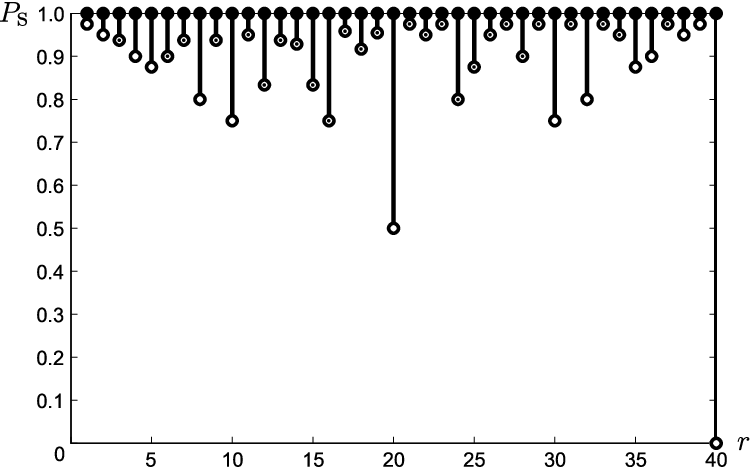
Fig. 6: Plot of the desired recovery probability PS{P_{\text{S}}} against the number of nodes accessed rr, showing intervals of PS{P_{\text{S}}} over which the allocation (1r,…,1r)\left(\frac{1}{r},\ldots,\frac{1}{r}\right) is optimal for 𝚷2′​(n,r,PS){\mathbf{\Pi}}^{\prime}_{2}(n,r,{P_{\text{S}}}), for n=40n=40. A dotted circle marker denotes an endpoint that may not be tight, i.e., we have not demonstrated that the allocation is suboptimal everywhere outside the interval.

Fig. 6 illustrates these results for an instance of nn.

By combining the proof techniques of Lemma 1 and Theorems 2, 5, and 6, we can derive the improved upper bound PSUBP_{\text{S}}^{\textsf{UB}}, given by (20) at the bottom of the page, for the recovery probability of an optimal allocation in the independent probabilistic access model of Section II (cf. Lemma 1). Variables α\alpha and r′r^{\prime} are uniquely defined integers satisfying

n−ℓ=α​r+r′,α∈ℤ0+,r′∈{r,…,2​r−1}.n-\ell=\alpha\,r+r^{\prime},\quad\alpha\in{\mathbb{Z}}^{+}_{0},\quad r^{\prime}\in\{r,\ldots,2r-1\}.

Parameter ℓ\ell denotes the number of individual nodes that store at least a unit amount of data. At least ℓ\ell amount of data is stored in these complete nodes, leaving the remaining budget of at most T−ℓT-\ell to be allocated over the remaining n−ℓn-\ell incomplete nodes. Term (i) gives the probability of successful recovery from accessing at least one complete node, while term (ii) gives an upper bound on the probability of successful recovery from accessing exactly r∈r\in {2,…,n−ℓ}\{2,\ldots,n-\ell\} incomplete nodes.

IV Probabilistic Symmetric Allocations

In the third variation of the storage allocation problem, we consider the case where each of the nn nodes is selected by the source independently with probability min⁡(ℓ​Tn,1)\min\!\left(\frac{\ell T}{n},1\right) to store 1ℓ\frac{1}{\ell} amount of data, so that the expected total amount of storage used in the resulting symmetric allocation is at most n⋅ℓ​Tn⋅1ℓn\cdot\frac{\ell T}{n}\cdot\frac{1}{\ell} =T=T, the given budget. The data collector subsequently accesses an rr-subset of the nn nodes selected uniformly at random from the collection of all (nr)\left(\genfrac{}{}{0.0pt}{}{n}{r}\right) possible rr-subsets, where rr is a given constant; successful recovery occurs if and only if the total amount of data stored in the accessed nodes is at least 11. We seek an optimal probabilistic symmetric allocation of the budget TT, specified by the value of parameter ℓ\ell, that maximizes the probability of successful recovery, for a given choice of nn, rr, and TT. Since successful recovery for a particular choice of ℓ\ell occurs if and only if at least ⌈1/(1ℓ)⌉{\left\lceil{1\big/\left(\frac{1}{\ell}\right)}\right\rceil} =⌈ℓ⌉={\left\lceil{\ell}\right\rceil} out of the rr accessed nodes are nonempty, the corresponding probability of successful recovery can be written as

PS(n,r,T,ℓ)≜ℙ[ℬ(r,min(ℓ​Tn,1))≥⌈ℓ⌉].\textstyle{P_{\text{S}}}(n,r,T,\ell)\triangleq{\mathbb{P}\left[{\mathcal{B}\left(r\vphantom{\Big|},\min\!\left(\frac{\ell T}{n},1\right)\right)}\geq{\left\lceil{\ell\vphantom{\big|}}\right\rceil}\right]}.

This optimization problem can therefore be expressed as follows:

𝚷3​(n,r,T):\displaystyle{\mathbf{\Pi}}_{3}(n,r,T):\hskip 170.00026pt
maximizeℓℙ[ℬ(r,min(ℓ​Tn,1))≥⌈ℓ⌉]\displaystyle\hskip 18.00005pt\underset{\ell}{\text{maximize}}\hskip 15.00002pt\textstyle{\mathbb{P}\left[{\mathcal{B}\left(r\vphantom{\Big|},\min\!\left(\frac{\ell T}{n},1\right)\right)}\geq{\left\lceil{\ell\vphantom{\big|}}\right\rceil}\right]}
subject toℓ>0.\displaystyle\hskip 18.99995pt\text{subject to}\hskip 13.99995pt\ell>0.

For budget T≥nrT\geq\frac{n}{r}, the choice of ℓ=r\ell=r, which yields a recovery probability of ℙ[ℬ(r,1)≥r]{\mathbb{P}\left[{\mathcal{B}\left(r,1\right)}\geq r\right]} =1=1, is optimal.

Observe that the recovery probability PS​(n,r,T,ℓ){P_{\text{S}}}(n,r,T,\ell) is zero when ℓ>r\ell>r. Furthermore, for fixed nn, rr, and TT, the recovery probability is nondecreasing in ℓ\ell within each of the unit intervals (0,1](0,1], (1,2](1,2], (2,3](2,3], …\ldots, since as ℓ\ell increases within each interval, ⌈ℓ⌉{\left\lceil{\ell}\right\rceil} remains constant while min⁡(ℓ​Tn,1)\min\!\left(\frac{\ell T}{n},1\right) either increases or remains constant at 11. Thus, given nn, rr, and TT, we can find an optimal ℓ∗\ell^{*} from among rr candidates:

{1,2,…,r}.\displaystyle\big\{1,2,\ldots,r\big\}. (21)
Refer to caption
Fig. 7: Plot of recovery probability PS{P_{\text{S}}} against budget-per-node Tn\frac{T}{n} for each choice of parameter ℓ∈{1,2,…,r}\ell\in\{1,2,\ldots,r\}, for r=10r=10. Parameter ℓ\ell controls how much the budget is spread in the probabilistic symmetric allocation; specifically, each of the nn nodes is selected by the source independently with probability min⁡(ℓ​Tn,1)\min\!\big(\frac{\ell T}{n},1\big) to store 1ℓ\frac{1}{\ell} amount of data. Arrows indicate the direction of increasing ℓ\ell. The black dashed line marks the threshold on Tn\frac{T}{n} derived in Theorem 7; maximal spreading (ℓ=r\ell=r) is optimal for any Tn\frac{T}{n} greater than or equal to this threshold.

Fig. 7, which compares the performance of different probabilistic symmetric allocations over different budgets for an instance of rr, suggests that there are two distinct phases pertaining to the optimal choice of ℓ\ell: when the budget is below a certain threshold, the choice of ℓ=1\ell=1, which corresponds to a minimal spreading of the budget (uncoded replication), is optimal; when the budget exceeds that same threshold, the choice of ℓ=r\ell=r, which corresponds to a maximal spreading of the budget, becomes optimal. This observation echoes our findings on the allocation and access models of the preceding sections, namely that minimal spreading (ℓ=1\ell=1) is optimal for sufficiently small budgets, while maximal spreading (ℓ=r\ell=r) is optimal for sufficiently large budgets. However, we note two important distinctions in contrast to the previous models. First, the recovery probability for a probabilistic symmetric allocation in this model is a continuous nondecreasing function of the given budget; there are no “jumps” from one discrete value to the next. Second, our empirical computations suggest that the phase transition from the optimality of minimal spreading to that of maximal spreading in this model is sharp; the other intermediate values of ℓ∈{2,…,r−1}\ell\in\{2,\ldots,r-1\} never perform better than both ℓ=1\ell=1 and ℓ=r\ell=r simultaneously.

In Section IV-A, we shall demonstrate that the choice of ℓ=r\ell=r, which corresponds to a maximal spreading of the budget, is indeed optimal when the given budget TT is sufficiently large, or equivalently, when a sufficiently high recovery probability is achievable.

IV-A Optimality of Maximal Spreading

Assume that r≥2r\geq 2. As noted earlier, the choice of ℓ=r\ell=r, which corresponds to a maximal spreading of the budget, is optimal for any T≥nrT\geq\frac{n}{r} because it yields the maximal recovery probability of 11. The following lemma provides an upper bound for the recovery probabilities corresponding to the other candidate values for ℓ∗\ell^{*} in (21) at the critical budget T=nrT=\frac{n}{r}:

Lemma 6.

The probability of successful recovery PS​(n,r,T,ℓ){P_{\text{S}}}(n,r,T,\ell) at T=nrT=\frac{n}{r} is at most 34\frac{3}{4} for any ℓ∈{1,2,…,r−1}\ell\in\{1,2,\ldots,r-1\}.

Such an upper bound allows us to derive a sufficient condition for the optimality of ℓ=r\ell=r, by making use of the fact that the recovery probability PS​(n,r,T,ℓ){P_{\text{S}}}(n,r,T,\ell) is a nondecreasing function of the budget TT. The following theorem shows that the choice of ℓ=r\ell=r is optimal when the budget TT is at least a specified threshold expressed in terms of nn and rr:

Theorem 7.

If

T≥nr​(34)1r,T\geq\frac{n}{r}\left(\frac{3}{4}\right)^{\frac{1}{r}},

then the choice of ℓ=r\ell=r, which corresponds to a maximal spreading of the budget, is optimal.

The following corollary states an equivalent result in terms of the achievable recovery probability; it demonstrates the optimality of ℓ=r\ell=r in the high recovery probability regime:

Corollary 4.

If a probability of successful recovery of at least 34\frac{3}{4} is achievable for the given nn, rr, and TT, then the choice of ℓ=r\ell=r is optimal.

Refer to caption
Fig. 8: Plot of recovery probability PS{P_{\text{S}}} against the number of nodes accessed rr, indicating the value of PS{P_{\text{S}}} at which the optimal choice of parameter ℓ\ell changes from 11 to rr, for each given value of rr. Specifically, if it is possible to achieve a recovery probability PS{P_{\text{S}}} above the square marker, then maximal spreading (ℓ=r\ell=r) is optimal; otherwise, minimal spreading or uncoded replication (ℓ=1\ell=1) is optimal. Observe that the critical value of PS{P_{\text{S}}} for r=10r=10 (which is approximately 0.6336520.633652) corresponds to the intersection point of the curves for ℓ=1\ell=1 and ℓ=10\ell=10 in Fig. 7.

Fig. 8 describes the optimal choice of ℓ\ell for different values of rr. We observe that the gap between the threshold of 34\frac{3}{4} derived in Corollary 4 and the actual critical value of PS{P_{\text{S}}} indicated in the plot appears to be no more than 0.120.12.

V Conclusion and Future Work

We examined the problem of allocating a given total storage budget in a distributed storage system for maximum reliability. Three variations of the problem were studied in detail, and we are able to specify the optimal allocation or optimal symmetric allocation for a variety of cases. Although the exact optimal allocation is difficult to find in general, our results suggest a simple heuristic for achieving reliable storage: when the budget is small, spread it minimally; when the budget is large, spread it maximally. In other words, coding is unnecessary when the budget is small, but is beneficial when the budget is large.

The work in this paper can be extended in several directions. We can impose additional system design constraints on the model; one practical example is the application of a tighter per-node storage constraint xi≤ci<1x_{i}\leq c_{i}<1. The independent probabilistic access model of Section II can be naturally generalized to the case of nonuniform access probabilities pip_{i} for individual nodes. It would also be interesting to find reliable allocations for specific codes with desirable encoding or decoding properties, e.g., sparse codes that offer efficient algorithms (see, e.g., [24, 25, 26, 27]). A related problem would be to construct such codes that work well under different allocations. Another set of interesting problems involves the application of richer access models; for instance, we can introduce a network topology to a set of storage nodes and data collectors, and allow each data collector to access only the nodes close to it. More generally, we can assign different priorities to each node for data storage and access, so as to reflect the costs of storing data in the node and communicating with it.

[Proofs of Theorems]

Proof:

We note that the computational complexity of this problem was well understood in the Berkeley meetings [9] and is by no means a major contribution in this paper. We present the detailed proofs here for completeness.

Consider an allocation (x1,…,xn)\left(x_{1},\ldots,x_{n}\right) where each xix_{i} is a nonnegative rational number. The problem of computing the recovery probability of this allocation for the special case of p=12p=\frac{1}{2}, for which p|𝐫|​(1−p)n−|𝐫|=(12)np^{|{\mathbf{r}}|}(1-p)^{n-|{\mathbf{r}}|}=\left(\frac{1}{2}\right)^{n} for any subset 𝐫⊆{1,…,n}{\mathbf{r}}\subseteq{{\mbox{$\left\{1,\ldots,n\right\}$}}}, is equivalent to the counting version of the following decision problem (which happens to be polynomial-time solvable):

Definition.

Largest Subset Sum (LSS)
Instance: Finite nn-vector (a1,…,an)\left(a_{1},\ldots,a_{n}\right) with ai∈ℤ0+a_{i}\in{\mathbb{Z}}^{+}_{0}, and file size d∈ℤ+d\in{\mathbb{Z}}^{+}, where all aia_{i} and dd can be written as decimal numbers of length at most ℓ\ell.
Question: Is there a subset 𝐫⊆{1,…,n}{\mathbf{r}}\subseteq{{\mbox{$\left\{1,\ldots,n\right\}$}}} that satisfies ∑i∈𝐫ai≥d\sum_{i\in{\mathbf{r}}}a_{i}\geq d?

Note that the allocation and file size have been scaled so that the problem parameters are all integers. We will proceed to show that the counting problem #LSS is #P-complete; this would in turn establish the #P-hardness of computing the recovery probability for an arbitrary value of pp.

The index set 𝐫{\mathbf{r}} can be represented as an nn-vector of bits. Using this representation of 𝐫{\mathbf{r}} as the certificate, it is easy to see that the binary relation corresponding to #LSS is both polynomially balanced (since the size of each certificate is nn), and polynomial-time decidable (since the inequality can be verified in O⁡(n​ℓ)O(n\ell) time for each certificate). It therefore follows that #LSS is in #P.

To show that #LSS is also #P-hard, we describe a polynomial-time Turing reduction of the #P-complete problem #3SAT [28] to #LSS. Our approach is similar to the standard method of reducing 3SAT to Subset Sum (see, e.g., [29]). Let ϕ\phi be the Boolean formula in the given #3SAT instance; denote its mm variables by v1,…,vmv_{1},\ldots,v_{m}, and kk clauses by C1,…,CkC_{1},\ldots,C_{k}. To count the number of satisfying truth assignments for ϕ\phi, we construct a #LSS instance with the help of Table III, whose entries are 00, 11, 22, or 33 (all blank entries are 00’s).

TABLE III: Constructing a #LSS instance for a given #3SAT instance
v1v_{1} v2v_{2} ⋯\cdots vmv_{m} C1C_{1} C2C_{2} ⋯\cdots CkC_{k}
v1v_{1} 11 1[v1∈C1]{\mathbbold{1}\left[v_{1}{\in}C_{1}\right]} 00 1[v1∈C2]{\mathbbold{1}\left[v_{1}{\in}C_{2}\right]} 00 ⋯\cdots 1[v1∈Ck]{\mathbbold{1}\left[v_{1}{\in}C_{k}\right]} 00
v1¯\overline{v_{1}} 11 1[v1¯∈C1]{\mathbbold{1}\left[\overline{v_{1}}{\in}C_{1}\right]} 00 1[v1¯∈C2]{\mathbbold{1}\left[\overline{v_{1}}{\in}C_{2}\right]} 00 ⋯\cdots 1[v1¯∈Ck]{\mathbbold{1}\left[\overline{v_{1}}{\in}C_{k}\right]} 00
[2pt/3pt]v2v_{2} 11 1[v2∈C1]{\mathbbold{1}\left[v_{2}{\in}C_{1}\right]} 00 1[v2∈C2]{\mathbbold{1}\left[v_{2}{\in}C_{2}\right]} 00 ⋯\cdots 1[v2∈Ck]{\mathbbold{1}\left[v_{2}{\in}C_{k}\right]} 00
v2¯\overline{v_{2}} 11 1[v2¯∈C1]{\mathbbold{1}\left[\overline{v_{2}}{\in}C_{1}\right]} 00 1[v2¯∈C2]{\mathbbold{1}\left[\overline{v_{2}}{\in}C_{2}\right]} 00 ⋯\cdots 1[v2¯∈Ck]{\mathbbold{1}\left[\overline{v_{2}}{\in}C_{k}\right]} 00
[2pt/3pt]⋮\vdots ⋱\ddots ⋮\vdots ⋮\vdots ⋮\vdots ⋮\vdots ⋮\vdots ⋮\vdots ⋮\vdots
[2pt/3pt]vmv_{m} 11 1[vm∈C1]{\mathbbold{1}\left[v_{m}{\in}C_{1}\right]} 00 1[vm∈C2]{\mathbbold{1}\left[v_{m}{\in}C_{2}\right]} 00 ⋯\cdots 1[vm∈Ck]{\mathbbold{1}\left[v_{m}{\in}C_{k}\right]} 00
vm¯\overline{v_{m}} 11 1[vm¯∈C1]{\mathbbold{1}\left[\overline{v_{m}}{\in}C_{1}\right]} 00 1[vm¯∈C2]{\mathbbold{1}\left[\overline{v_{m}}{\in}C_{2}\right]} 00 ⋯\cdots 1[vm¯∈Ck]{\mathbbold{1}\left[\overline{v_{m}}{\in}C_{k}\right]} 00
C1C_{1} 00 11
11 11
22 11
[2pt/3pt]C2C_{2} 00 11
11 11
22 11
[2pt/3pt]⋮\vdots ⋱\ddots
[2pt/3pt]CkC_{k} 00 11
11 11
22 11
 
dd 11 11 ⋯\cdots 11 33 11 33 11 ⋯\cdots 33 11

The entries of the nn-vector for the #LSS instance are given by the first (2​m+3​k)(2m+3k) rows of the table; the file size dd is given by the last row of the table. Each entry aia_{i}, i∈{1,…,2​m+3​k}i\in\{1,\ldots,2m+3k\}, as well as dd, is a positive integer with at most (m+2​k)(m+2k) decimal digits. Observe that the set of satisfying truth assignments for ϕ\phi can be put in a one-to-one correspondence with the collection of subsets 𝐫⊆{1,…,2​m+3​k}{\mathbf{r}}\subseteq\{1,\ldots,2m+3k\} that satisfy ∑i∈𝐫ai=d\sum_{i\in{\mathbf{r}}}a_{i}=d; for each i∈{1,…,m}i\in\{1,\ldots,m\}, we have “viv_{i}” ∈𝐫\in{\mathbf{r}} if and only if vi=v_{i}= true, and “vi¯\overline{v_{i}}” ∈𝐫\in{\mathbf{r}} if and only if vi=v_{i}= false. Therefore, if f⁡((a1,…,an),d)f\big((a_{1},\ldots,a_{n}),d\big) is a subroutine for computing #LSS, then the number of satisfying truth assignments can be computed by calling ff twice: first with dd taking the value as prescribed above, and second with dd taking the prescribed value plus one. The difference between the outputs from the two subroutine calls is equal to the number of distinct subsets 𝐫{\mathbf{r}} that satisfy ∑i∈𝐫ai=d\sum_{i\in{\mathbf{r}}}a_{i}=d, which is equal to the number of satisfying truth assignments for ϕ\phi. Finally, we note that this is indeed a polynomial-time Turing reduction since the table can be populated in O⁡(m2​k2)O\left(m^{2}k^{2}\right) simple steps, and the subroutine ff is called exactly twice. ∎

Proof:

Consider a feasible allocation (x1,…,xn)\left(x_{1},\ldots,x_{n}\right); we have ∑i=1nxi≤T\sum_{i=1}^{n}x_{i}\leq T, where xi≥0x_{i}\geq 0, i=1,…,ni=1,\ldots,n. Let SrS_{r} denote the number of rr-subsets of {x1,…,xn}\{x_{1},\ldots,x_{n}\} that have a sum of at least 11, where r∈{1,…,n}r\in{{\mbox{$\left\{1,\ldots,n\right\}$}}}. By conditioning on the number of nodes accessed by the data collector, the probability of successful recovery for this allocation can be written as

ℙ⁡[successful recovery]\displaystyle{\mathbb{P}\left[\text{successful recovery}\right]}
=∑r=1nℙ[successful recovery|exactly r nodes were accessed]⋅ℙ⁡[exactly r nodes were accessed]\displaystyle\hskip-1.99997pt=\hskip-1.99997pt\sum_{r=1}^{n}\hskip-5.0pt\begin{array}[]{l}{\mathbb{P}\left[\text{successful recovery}\,|\,\text{exactly $r$ nodes were accessed}\right]}\cdot\\ \hskip 85.50015pt{\mathbb{P}\left[\text{exactly $r$ nodes were accessed}\right]}\end{array}
=∑r=1nSr(nr)⋅ℙ[ℬ(n,p)=r].\displaystyle\hskip-1.99997pt=\hskip-1.99997pt\sum_{r=1}^{n}\frac{S_{r}}{\left(\genfrac{}{}{0.0pt}{}{n}{r}\right)}\cdot{\mathbb{P}\left[{\mathcal{B}\left(n,p\right)}=r\right]}. (24)

We proceed to find an upper bound for SrS_{r}. For a given rr, we can write SrS_{r} inequalities of the form

x1′+⋯+xr′≥1.x^{\prime}_{1}+\cdots+x^{\prime}_{r}\geq 1.

Summing up these SrS_{r} inequalities produces an inequality of the form

a1​x1+⋯+an​xn≥Sr.a_{1}x_{1}+\cdots+a_{n}x_{n}\geq S_{r}.

Since each xix_{i} belongs to exactly (n−1r−1)\left(\genfrac{}{}{0.0pt}{}{n-1}{r-1}\right) distinct rr-subsets of {x1,…,xn}\left\{x_{1},\ldots,x_{n}\right\}, it follows that 0≤ai≤(n−1r−1)0\leq a_{i}\leq\left(\genfrac{}{}{0.0pt}{}{n-1}{r-1}\right), i=1,…,ni=1,\ldots,n. Therefore,

Sr≤a1​x1+⋯+an​xn\displaystyle S_{r}\leq a_{1}x_{1}+\cdots+a_{n}x_{n}
≤(n−1r−1)​∑i=1nxi≤(n−1r−1)​T.\displaystyle\hskip 70.0001pt\leq\left(\genfrac{}{}{0.0pt}{}{n-1}{r-1}\right)\sum_{i=1}^{n}x_{i}\leq\left(\genfrac{}{}{0.0pt}{}{n-1}{r-1}\right)T.

Since SrS_{r} is also at most (nr)\left(\genfrac{}{}{0.0pt}{}{n}{r}\right), i.e., the total number of rr-subsets, we have

Sr≤min⁡((n−1r−1)​T,(nr)).S_{r}\leq\min\left(\left(\genfrac{}{}{0.0pt}{}{n-1}{r-1}\right)T,\left(\genfrac{}{}{0.0pt}{}{n}{r}\right)\right).

Substituting this bound into (24) completes the proof. ∎

Proof:

The suboptimality gap for the symmetric allocation 𝐱¯​(n,T,m=n){\bar{\mathbf{x}}}\left(n,T,m{=}n\right) is at most the difference between its recovery probability (5) and the upper bound (6) from Lemma 1 for the optimal recovery probability. This difference is given by

∑r=1⌈nT⌉−1r​Tn​(nr)​pr​(1−p)n−r\displaystyle\quad\sum_{r=1}^{{\left\lceil{\frac{n}{T}}\right\rceil}-1}\frac{rT}{n}\left(\genfrac{}{}{0.0pt}{}{n}{r}\right)p^{r}(1-p)^{n-r}
=T​∑r=1⌈nT⌉−1(n−1r−1)​pr​(1−p)n−r\displaystyle=T\;\sum_{r=1}^{{\left\lceil{\frac{n}{T}}\right\rceil}-1}\left(\genfrac{}{}{0.0pt}{}{n-1}{r-1}\right)p^{r}(1-p)^{n-r}
=p​T​∑r=1⌈nT⌉−1(n−1r−1)​pr−1​(1−p)(n−1)−(r−1)\displaystyle=p\,T\;\sum_{r=1}^{{\left\lceil{\frac{n}{T}}\right\rceil}-1}\left(\genfrac{}{}{0.0pt}{}{n-1}{r-1}\right)p^{r-1}(1-p)^{(n-1)-(r-1)}
=p​T​∑ℓ=0⌈nT⌉−2(n−1ℓ)​pℓ​(1−p)(n−1)−ℓ\displaystyle=p\,T\;\sum_{\ell=0}^{{\left\lceil{\frac{n}{T}}\right\rceil}-2}\left(\genfrac{}{}{0.0pt}{}{n-1}{\ell}\right)p^{\ell}(1-p)^{(n-1)-\ell}
=pTℙ[ℬ(n−1,p)≤⌈nT⌉−2]≜δ(n,p,T),\displaystyle=p\,T\;{\mathbb{P}\left[\displaystyle{\mathcal{B}\left(n-1,p\right)}\leq{\left\lceil{\frac{n}{T}}\right\rceil}-2\right]}\;\triangleq\;\delta(n,p,T),

as required. Assuming now that p>1Tp>\frac{1}{T}, we have

δ⁡(n,p,T)\displaystyle\delta(n,p,T) ≤pTℙ[ℬ(n−1,p)≤n−1T]\displaystyle\leq p\,T\;{\mathbb{P}\left[\displaystyle{\mathcal{B}\left(n-1,p\right)}\leq\frac{n-1}{T}\right]} (25)
=pTℙ[ℬ(n−1,p)≤1p​T(n−1)p]\displaystyle=p\,T\;{\mathbb{P}\left[\displaystyle{\mathcal{B}\left(n-1,p\right)}\leq\frac{1}{pT}(n-1)p\right]}
≤p​T​exp⁡(−(n−1)​p2​(1−1p​T)2).\displaystyle\leq p\,T\;\exp\left(-\frac{(n-1)p}{2}\left(1-\frac{1}{pT}\right)^{2}\right). (26)

Inequality (25) follows from the fact that

⌈nT⌉−2<nT+1−2<nT−1T.{\left\lceil{\frac{n}{T}}\right\rceil}-2\;<\;\frac{n}{T}+1-2\;<\;\frac{n}{T}-\frac{1}{T}.

Inequality (26) follows from the observation that 1p​T∈(0,1)\frac{1}{pT}\in(0,1), and the subsequent application of the Chernoff bound for deviation below the mean of the binomial distribution (see, e.g., [30]). For fixed pp and TT, this upper bound approaches zero as nn goes to infinity. ∎

Proof:

We compare the recovery probability of 𝐱¯​(n,T,m=⌊T⌋){\bar{\mathbf{x}}}\left(n,T,m{=}{\left\lfloor{T}\right\rfloor}\right) to an upper bound for the recovery probabilities of all other allocations.

Suppose that 1<T<n1<T<n. Recall from (7) that the probability of successful recovery for 𝐱¯​(n,T,m=⌊T⌋){\bar{\mathbf{x}}}\left(n,T,m{=}{\left\lfloor{T}\right\rfloor}\right) is given by

P1​(p,T)≜1−(1−p)⌊T⌋.P_{1}(p,T)\triangleq 1-(1-p)^{{\left\lfloor{T}\right\rfloor}}.

Consider a feasible allocation (x1,…,xn)\left(x_{1},\ldots,x_{n}\right); we have ∑i=1nxi≤T\sum_{i=1}^{n}x_{i}\leq T, where xi≥0x_{i}\geq 0, i=1,…,ni=1,\ldots,n. Let ℓ\ell be the number of individual nodes in this allocation that store at least a unit amount of data; for brevity, we refer to these nodes as being complete. It follows from the budget constraint that the number of complete nodes ℓ∈\ell\in {0,1,…,⌊T⌋}\{0,1,\ldots,{\left\lfloor{T}\right\rfloor}\}. When ℓ=⌊T⌋\ell={\left\lfloor{T}\right\rfloor}, the allocation has a recovery probability identical to P1​(p,T)P_{1}(p,T). Now, assuming that ℓ∈\ell\in {0,1,…,⌊T⌋−1}\{0,1,\ldots,{\left\lfloor{T}\right\rfloor}-1\}, successful recovery can occur in two ways:

  1. (i)

    when the accessed subset contains one or more complete nodes, which occurs with probability 1−(1−p)ℓ1-(1-p)^{\ell}, or

  2. (ii)

    when the accessed subset contains no complete nodes but has a sum of at least 11.

In case (ii), the accessed subset would consist of two or more incomplete nodes. Using the argument in the proof of Lemma 1, we can show that there are at most

min⁡((n−ℓ−1r−1)​(T−ℓ),(n−ℓr))\min\left(\left(\genfrac{}{}{0.0pt}{}{n-\ell-1}{r-1}\right)(T-\ell),\left(\genfrac{}{}{0.0pt}{}{n-\ell}{r}\right)\right)

rr-subsets of incomplete nodes whose sum is at least 11, since the total amount of data stored over the n−ℓn-\ell incomplete nodes is at most T−ℓT-\ell. It follows then that the recovery probability for a feasible allocation with exactly ℓ∈\ell\in {0,1,…,⌊T⌋−1}\{0,1,\ldots,{\left\lfloor{T}\right\rfloor}-1\} complete nodes is at most

P2(n,p,T,ℓ)≜1−(1−p)ℓ+(1−p)ℓ⋅\displaystyle P_{2}(n,p,T,\ell)\triangleq 1-(1-p)^{\ell}+(1-p)^{\ell}\cdot
∑r=2n−ℓmin⁡(T−ℓn−ℓ⋅r,1)​(n−ℓr)​pr​(1−p)n−ℓ−r.\displaystyle\quad\qquad\sum_{r=2}^{n-\ell}\min\left(\frac{T-\ell}{n-\ell}\cdot r,1\right)\left(\genfrac{}{}{0.0pt}{}{n-\ell}{r}\right)p^{r}(1-p)^{n-\ell-r}.

Thus,

P1​(p,T)≥P2​(n,p,T,ℓ)P_{1}(p,T)\geq P_{2}(n,p,T,\ell)

for all ℓ∈\ell\in {0,1,…,⌊T⌋−1}\{0,1,\ldots,{\left\lfloor{T}\right\rfloor}-1\} is a sufficient condition for 𝐱¯​(n,T,m=⌊T⌋){\bar{\mathbf{x}}}\left(n,T,m{=}{\left\lfloor{T}\right\rfloor}\right) to be an optimal allocation. After further simplification of this inequality, we arrive at inequality (8) as required. ∎

Proof:

Suppose that 1<T<n1<T<n. We will show that the sufficient condition of Theorem 2 is satisfied for any p≤2(n−⌊T⌋)2p\leq\frac{2}{\left(n-{\left\lfloor{T}\right\rfloor}\right)^{2}}. Note that when n−⌊T⌋=1n-{\left\lfloor{T}\right\rfloor}=1, or equivalently T∈[n−1,n)T\in[n-1,n), we have to show that 𝐱¯​(n,T,m=⌊T⌋){\bar{\mathbf{x}}}\left(n,T,m{=}{\left\lfloor{T}\right\rfloor}\right) is an optimal allocation for any pp, i.e., in the interval (0,1)(0,1).

First, observe that the summation term in inequality (8) is always nonnegative, i.e.,

∑r=2⌈n−ℓT−ℓ⌉−1(1−T−ℓn−ℓ⋅r)​(n−ℓr)​(p1−p)r≥0,\sum_{r=2}^{{\left\lceil{\frac{n-\ell}{T-\ell}}\right\rceil}-1}\left(1-\frac{T-\ell}{n-\ell}\cdot r\right)\left(\genfrac{}{}{0.0pt}{}{n-\ell}{r}\right)\left(\frac{p}{1-p}\right)^{r}\geq 0,

since for any r∈r\in {2,…,⌈n−ℓT−ℓ⌉−1}\left\{2,\ldots,{\left\lceil{\frac{n-\ell}{T-\ell}}\right\rceil}-1\right\} and ℓ∈\ell\in {0,1,…,⌊T⌋−1}\{0,1,\ldots,{\left\lfloor{T}\right\rfloor}-1\}, we have

r≤⌈n−ℓT−ℓ⌉−1⟺r<n−ℓT−ℓ⟺1−T−ℓn−ℓ⋅r>0.r\leq{\left\lceil{\frac{n-\ell}{T-\ell}}\right\rceil}-1\Longleftrightarrow r<\frac{n-\ell}{T-\ell}\Longleftrightarrow 1-\frac{T-\ell}{n-\ell}\cdot r>0.

Therefore, a simpler but weaker sufficient condition for 𝐱¯​(n,T,m=⌊T⌋){\bar{\mathbf{x}}}\left(n,T,m{=}{\left\lfloor{T}\right\rfloor}\right) to be an optimal allocation is

1−(1−p)⌊T⌋−n+(n−(⌊T⌋−1))​(p1−p)≥0\displaystyle 1-(1-p)^{{\left\lfloor{T}\right\rfloor}-n}+\left(n-\left({\left\lfloor{T}\right\rfloor}-1\right)\right)\left(\frac{p}{1-p}\right)\geq 0
⟺\displaystyle\Longleftrightarrow 1+(n−⌊T⌋)​p−(1−p)1−(n−⌊T⌋)≥0,\displaystyle 1+\left(n-{\left\lfloor{T}\right\rfloor}\right)p-(1-p)^{1-\left(n-{\left\lfloor{T}\right\rfloor}\right)}\geq 0,

which is an inequality in only two variables pp and s≜n−⌊T⌋s\triangleq n-{\left\lfloor{T}\right\rfloor}, where s∈s\in {1,…,n−1}\{1,\ldots,n-1\}. When s=1s=1, or equivalently T∈[n−1,n)T\in[n-1,n), this inequality is satisfied for any p∈(0,1)p\in(0,1), as required. Defining the function

f⁡(s,p)≜1+s​p−(1−p)1−s,f(s,p)\triangleq 1+s\,p-(1-p)^{1-s},

it suffices to show that f⁡(s,p)≥0f(s,p)\geq 0 for any s∈ℤ+s\in{\mathbb{Z}}^{+}, s≥2s\geq 2, and p∈(0,2s2]p\in\left(0,\frac{2}{s^{2}}\right]. We do this by demonstrating that for any s∈ℤ+s\in{\mathbb{Z}}^{+}, s≥2s\geq 2, the function f⁡(s,p)f(s,p) is concave in pp on the interval p∈(0,2s2]p\in\left(0,\frac{2}{s^{2}}\right], and is nonnegative at both endpoints, i.e., f⁡(s,p=0)≥0f(s,p{=}0)\geq 0 and f⁡(s,p=2s2)≥0f\left(s,p{=}\frac{2}{s^{2}}\right)\geq 0.

The second-order partial derivative of f⁡(s,p)f(s,p) wrt pp is given by

∂2∂p2​f​(s,p)=−s⁡(s−1)​(1−p)−1−s.\frac{\partial^{2}}{\partial p^{2}}f(s,p)=-s(s-1)(1-p)^{-1-s}.

Since ∂2∂p2​f​(s,p)<0\frac{\partial^{2}}{\partial p^{2}}f(s,p)<0 for any s∈ℤ+s\in{\mathbb{Z}}^{+}, s≥2s\geq 2, and p∈(0,2s2]p\in\left(0,\frac{2}{s^{2}}\right], it follows that the function f⁡(s,p)f(s,p) is concave in pp on the interval p∈(0,2s2]p\in\left(0,\frac{2}{s^{2}}\right] for any s∈ℤ+s\in{\mathbb{Z}}^{+}, s≥2s\geq 2.

Suppose that s∈ℤ+s\in{\mathbb{Z}}^{+}, s≥2s\geq 2. Clearly, f⁡(s,p=0)=0f(s,p{=}0)=0. To show that f⁡(s,p=2s2)≥0f\left(s,p{=}\frac{2}{s^{2}}\right)\geq 0, we define the function

g⁡(s)≜ln⁡(1+2s)+(s−1)​ln⁡(1−2s2),g(s)\triangleq\ln\left(1+\frac{2}{s}\right)+(s-1)\ln\left(1-\frac{2}{s^{2}}\right),

and show that g⁡(s)≥0g(s)\geq 0 for any s∈ℤ+s\in{\mathbb{Z}}^{+}, s≥2s\geq 2. Direct evaluation of the function gives us g⁡(s=2)=0g(s{=}2)=0, and g⁡(s=3)=g(s{=}3)= ln⁡53−2​ln⁡97>0\ln\frac{5}{3}-2\ln\frac{9}{7}>0. For s≥4s\geq 4, we consider the derivatives of g⁡(s)g(s):

g′​(s)\displaystyle g^{\prime}(s) =1s+1s+2−2​(s−2)s2−2+ln⁡(1−2s2),\displaystyle=\frac{1}{s}+\frac{1}{s+2}-\frac{2(s-2)}{s^{2}-2}+\ln\left(1-\frac{2}{s^{2}}\right),
g′′​(s)\displaystyle g^{\prime\prime}(s) =8​(s3−s2−6​s−2)s2​(s+2)2​(s2−2)2.\displaystyle=\frac{8\left(s^{3}-s^{2}-6s-2\right)}{s^{2}(s+2)^{2}\left(s^{2}-2\right)^{2}}.

Since g′′​(s)≥0g^{\prime\prime}(s)\geq 0 for any s≥4s\geq 4, and lims→∞g′​(s)=0\lim_{s\rightarrow\infty}g^{\prime}(s)=0, it follows that g′​(s)≤0g^{\prime}(s)\leq 0 for any s≥4s\geq 4. Now, since g′​(s)≤0g^{\prime}(s)\leq 0 for any s≥4s\geq 4, and lims→∞g⁡(s)=0\lim_{s\rightarrow\infty}g(s)=0, it follows that g⁡(s)≥0g(s)\geq 0 for any s≥4s\geq 4. Therefore, for any s∈ℤ+s\in{\mathbb{Z}}^{+}, s≥2s\geq 2, we have

ln⁡(1+2s)+(s−1)​ln⁡(1−2s2)=g⁡(s)≥0\displaystyle\ln\left(1+\frac{2}{s}\right)+(s-1)\ln\left(1-\frac{2}{s^{2}}\right)=g(s)\geq 0
⟺\displaystyle\Longleftrightarrow 1+2s≥(1−2s2)1−s\displaystyle 1+\frac{2}{s}\geq\left(1-\frac{2}{s^{2}}\right)^{1-s}
⟺\displaystyle\Longleftrightarrow f⁡(s,p=2s2)≥0,\displaystyle f\left(s,p{=}\frac{2}{s^{2}}\right)\geq 0,

as required. ∎

Proof:

We will show that if condition (11) is satisfied, then Δ⁡(p,T,k)≥0\Delta(p,T,k)\geq 0 for any k∈ℤ+k\in{\mathbb{Z}}^{+}. First, we note that

(⌊k​T⌋k−1)(⌊k​T⌋k)\displaystyle\frac{\left(\genfrac{}{}{0.0pt}{}{\floor{kT}}{k-1}\right)}{\left(\genfrac{}{}{0.0pt}{}{\floor{kT}}{k}\right)} =k⌊k​T⌋−k+1\displaystyle=\frac{k}{{\left\lfloor{kT}\right\rfloor}-k+1}
=k⌊k⁡(⌊T⌋+τ)⌋−k+1,where ​τ≜T−⌊T⌋∈[0,1)\displaystyle=\frac{k}{{\left\lfloor{k({\left\lfloor{T}\right\rfloor}+\tau)}\right\rfloor}-k+1},{\small\hskip-4.62497pt\begin{array}[]{l}\text{where }\tau\triangleq T-{\left\lfloor{T}\right\rfloor}\in[0,1)\end{array}}
=kk⁡⌊T⌋+⌊k​τ⌋−k+1\displaystyle=\frac{k}{k{\left\lfloor{T}\right\rfloor}+{\left\lfloor{k\tau}\right\rfloor}-k+1}
≥kk​⌊T⌋\displaystyle\geq\frac{k}{k{\left\lfloor{T}\right\rfloor}} (28)
=1⌊T⌋.\displaystyle=\frac{1}{{\left\lfloor{T}\right\rfloor}}. (29)

Inequality (28) follows from the fact that

⌊k​τ⌋≤k​τ<k⟺⌊k​τ⌋≤k−1⟺⌊k​τ⌋−k+1≤0.{\left\lfloor{k\tau}\right\rfloor}\leq k\tau<k\;\Longleftrightarrow\;{\left\lfloor{k\tau}\right\rfloor}\leq k-1\;\Longleftrightarrow\;{\left\lfloor{k\tau}\right\rfloor}-k+1\leq 0.

Now, if condition (11) is satisfied, then we necessarily have T≥2T\geq 2; otherwise, T∈[1,2)T\in[1,2) would imply that ⌊T⌋=1{\left\lfloor{T}\right\rfloor}=1, which produces (1−p)⌊T⌋+2​⌊T⌋​p​(1−p)⌊T⌋−1−1(1-p)^{{\left\lfloor{T}\right\rfloor}}+2{\left\lfloor{T}\right\rfloor}p(1-p)^{{\left\lfloor{T}\right\rfloor}-1}-1 =p>0=p>0, contradicting our assumption. It follows that

(1−p)⌊T⌋+2​⌊T⌋​p​(1−p)⌊T⌋−1−1≤0\displaystyle\qquad\;(1-p)^{{\left\lfloor{T}\right\rfloor}}+2{\left\lfloor{T}\right\rfloor}p(1-p)^{{\left\lfloor{T}\right\rfloor}-1}-1\leq 0
⟺ℙ[ℬ(⌊T⌋,p)=0]+2ℙ[ℬ(⌊T⌋,p)=1]−1≤0\displaystyle\Longleftrightarrow{\mathbb{P}\left[{\mathcal{B}\left({\left\lfloor{T}\right\rfloor},p\right)}=0\right]}+2{\mathbb{P}\left[{\mathcal{B}\left({\left\lfloor{T}\right\rfloor},p\right)}=1\right]}-1\leq 0
⟺ℙ[ℬ(⌊T⌋,p)≥2]≥ℙ[ℬ(⌊T⌋,p)=1]\displaystyle\Longleftrightarrow{\mathbb{P}\left[{\mathcal{B}\left({\left\lfloor{T}\right\rfloor},p\right)}\geq 2\right]}\geq{\mathbb{P}\left[{\mathcal{B}\left({\left\lfloor{T}\right\rfloor},p\right)}=1\right]}
⟺∑j=2⌊T⌋(⌊T⌋j)​pj​(1−p)⌊T⌋−j≥⌊T⌋​p​(1−p)⌊T⌋−1\displaystyle\Longleftrightarrow\sum_{j=2}^{{\left\lfloor{T}\right\rfloor}}\left(\genfrac{}{}{0.0pt}{}{\floor{T}}{j}\right)p^{j}(1-p)^{{\left\lfloor{T}\right\rfloor}-j}\geq{\left\lfloor{T}\right\rfloor}p(1-p)^{{\left\lfloor{T}\right\rfloor}-1}
⟺∑j=2⌊T⌋1⌊T⌋​(⌊T⌋j)​(p1−p)j−1≥1\displaystyle\Longleftrightarrow\sum_{j=2}^{{\left\lfloor{T}\right\rfloor}}\frac{1}{{\left\lfloor{T}\right\rfloor}}\left(\genfrac{}{}{0.0pt}{}{\floor{T}}{j}\right)\left(\frac{p}{1-p}\right)^{j-1}\geq 1 (30)
⟹∑j=2⌈T⌉1⌊T⌋​(⌈T⌉j)​(p1−p)j−1≥1.\displaystyle\Longrightarrow\sum_{j=2}^{{\left\lceil{T}\right\rceil}}\frac{1}{{\left\lfloor{T}\right\rfloor}}\left(\genfrac{}{}{0.0pt}{}{\ceil{T}}{j}\right)\left(\frac{p}{1-p}\right)^{j-1}\geq 1. (31)

Observe that αk,T≜⌊(k+1)​T⌋−⌊k​T⌋\alpha_{k,T}\triangleq{\left\lfloor{(k+1)T}\right\rfloor}-{\left\lfloor{kT}\right\rfloor} ∈{⌊T⌋,⌈T⌉}\in\left\{{\left\lfloor{T}\right\rfloor},{\left\lceil{T}\right\rceil}\right\}, because αk,T∈(T−1,T+1)\alpha_{k,T}\in\big(T-1,T+1\big) and there are only two integers ⌊T⌋{\left\lfloor{T}\right\rfloor} and ⌈T⌉{\left\lceil{T}\right\rceil}, which are possibly nondistinct, in this interval. It follows from (30) and (31) that

∑j=2αk,T1⌊T⌋​(αk,Tj)​(p1−p)j−1≥1.\displaystyle\sum_{j=2}^{\alpha_{k,T}}\frac{1}{{\left\lfloor{T}\right\rfloor}}\left(\genfrac{}{}{0.0pt}{}{\alpha_{k,T}}{j}\right)\left(\frac{p}{1-p}\right)^{j-1}\geq 1. (32)

Therefore, we have

∑i=1min⁡(αk,T−1,k)∑j=i+1αk,T(⌊k​T⌋k−i)(⌊k​T⌋k)​(αk,Tj)​(p1−p)−i+j\displaystyle\sum_{i=1}^{\min(\alpha_{k,T}-1,k)}\sum_{j=i+1}^{\alpha_{k,T}}\frac{\left(\genfrac{}{}{0.0pt}{}{\floor{kT}}{k-i}\right)}{\left(\genfrac{}{}{0.0pt}{}{\floor{kT}}{k}\right)}\left(\genfrac{}{}{0.0pt}{}{\alpha_{k,T}}{j}\right)\left(\frac{p}{1-p}\right)^{-i+j}
≥∑i=11∑j=i+1αk,T(⌊k​T⌋k−i)(⌊k​T⌋k)​(αk,Tj)​(p1−p)−i+j\displaystyle\quad\!\geq\sum_{i=1}^{1}\sum_{j=i+1}^{\alpha_{k,T}}\frac{\left(\genfrac{}{}{0.0pt}{}{\floor{kT}}{k-i}\right)}{\left(\genfrac{}{}{0.0pt}{}{\floor{kT}}{k}\right)}\left(\genfrac{}{}{0.0pt}{}{\alpha_{k,T}}{j}\right)\!\left(\frac{p}{1-p}\right)^{\!\!-i+j} (33)
=∑j=2αk,T(⌊k​T⌋k−1)(⌊k​T⌋k)​(αk,Tj)​(p1−p)j−1\displaystyle\quad\!=\sum_{j=2}^{\alpha_{k,T}}\frac{\left(\genfrac{}{}{0.0pt}{}{\floor{kT}}{k-1}\right)}{\left(\genfrac{}{}{0.0pt}{}{\floor{kT}}{k}\right)}\left(\genfrac{}{}{0.0pt}{}{\alpha_{k,T}}{j}\right)\left(\frac{p}{1-p}\right)^{j-1}
≥∑j=2αk,T1⌊T⌋​(αk,Tj)​(p1−p)j−1, from (29)\displaystyle\quad\!\geq\sum_{j=2}^{\alpha_{k,T}}\frac{1}{{\left\lfloor{T}\right\rfloor}}\left(\genfrac{}{}{0.0pt}{}{\alpha_{k,T}}{j}\right)\left(\frac{p}{1-p}\right)^{j-1},\text{ from \eqref{eq:MaxBinomFrac}}
≥1, from (32).\displaystyle\quad\!\geq 1,\text{ from \eqref{eq:MaxAlphaSum}}.

Inequality (33) follows from the fact that

min⁡(αk,T−1,k)≥min⁡(2−1,1)= 1.\min(\alpha_{k,T}{-}1,k)\;\geq\;\min(2{-}1,1)\;=\;1.

Consequently,

∑i=1min⁡(αk,T−1,k)∑j=i+1αk,T(⌊k​T⌋k−i)​(αk,Tj)​(p1−p)−i+j≥(⌊k​T⌋k)\displaystyle\sum_{i=1}^{\min(\alpha_{k,T}-1,k)}\sum_{j=i+1}^{\alpha_{k,T}}\left(\genfrac{}{}{0.0pt}{}{\floor{kT}}{k-i}\right)\left(\genfrac{}{}{0.0pt}{}{\alpha_{k,T}}{j}\right)\left(\frac{p}{1-p}\right)^{-i+j}\geq\left(\genfrac{}{}{0.0pt}{}{\floor{kT}}{k}\right)
⟺Δ⁡(p,T,k)≥0, from (II-C).\displaystyle{\normalsize\begin{array}[]{l}\displaystyle\Longleftrightarrow\Delta(p,T,k)\geq 0,\text{ from \eqref{eq:DeltaK}}.\end{array}}

It follows that

PS​(p,T,m=⌊T⌋)≤PS​(p,T,m=⌊2​T⌋)\displaystyle{{\mbox{${P_{\text{S}}}\left(p,T,m{=}{\left\lfloor{T}\right\rfloor}\right)$}}}\leq{{\mbox{${P_{\text{S}}}\left(p,T,m{=}{\left\lfloor{2T}\right\rfloor}\right)$}}}
≤⋯≤PS​(p,T,m=⌊⌊nT⌋​T⌋),\displaystyle\hskip 100.00015pt\leq\cdots\leq{{\mbox{${P_{\text{S}}}\left(p,T,m{=}{\left\lfloor{{\left\lfloor{\frac{n}{T}}\right\rfloor}T}\right\rfloor}\right)$}}},

and so we conclude that an optimal m∗m^{*} is given by either m=⌊⌊nT⌋​T⌋m={\left\lfloor{{\left\lfloor{\frac{n}{T}}\right\rfloor}T}\right\rfloor} or m=nm=n. ∎

Proof:

If p≥43​⌊T⌋p\geq\frac{4}{3{\left\lfloor{T}\right\rfloor}}, then we necessarily have T≥2T\geq 2; otherwise, T∈[1,2)T\in[1,2) would imply that ⌊T⌋=1{\left\lfloor{T}\right\rfloor}=1, which produces p≥43​⌊T⌋p\geq\frac{4}{3{\left\lfloor{T}\right\rfloor}} =43=\frac{4}{3}, contradicting the definition of pp. We will show that condition (11) of Theorem 3 is satisfied for any T≥2T\geq 2 and p≥43​⌊T⌋p\geq\frac{4}{3{\left\lfloor{T}\right\rfloor}}. To do this, we define the function

f⁡(p,T)≜(1−p)⌊T⌋+2​⌊T⌋​p​(1−p)⌊T⌋−1−1,f(p,T)\triangleq(1-p)^{{\left\lfloor{T}\right\rfloor}}+2{\left\lfloor{T}\right\rfloor}p(1-p)^{{\left\lfloor{T}\right\rfloor}-1}-1,

and show that f⁡(p,T)≤f⁡(p=43​⌊T⌋,T)≤0f(p,T)\leq f\left(p{=}\frac{4}{3{\left\lfloor{T}\right\rfloor}},T\right)\leq 0 for any T≥2T\geq 2 and p≥43​⌊T⌋p\geq\frac{4}{3{\left\lfloor{T}\right\rfloor}}.

The partial derivative of f⁡(p,T)f(p,T) wrt pp is given by

∂∂p​f​(p,T)=⌊T⌋​(1−p)⌊T⌋−2​(1+p−2​⌊T⌋​p).\frac{\partial}{\partial p}f(p,T)={\left\lfloor{T}\right\rfloor}(1-p)^{{\left\lfloor{T}\right\rfloor}-2}\left(1+p-2{\left\lfloor{T}\right\rfloor}p\right).

Observe that f⁡(p,T)f(p,T) is decreasing wrt pp for any T≥2T\geq 2 and p≥43​⌊T⌋p\geq\frac{4}{3{\left\lfloor{T}\right\rfloor}}, since

p≥43​⌊T⌋=134​⌊T⌋>12​⌊T⌋−1\displaystyle\hskip 20.00003ptp\geq\frac{4}{3{\left\lfloor{T}\right\rfloor}}=\frac{1}{\frac{3}{4}{\left\lfloor{T}\right\rfloor}}>\frac{1}{2{\left\lfloor{T}\right\rfloor}-1}
⟹2​⌊T⌋​p−p>1⟺1+p−2​⌊T⌋​p<0⟺∂∂p​f​(p,T)<0.\displaystyle{\small\hskip-4.62497pt\begin{array}[]{l}\Longrightarrow 2{\left\lfloor{T}\right\rfloor}p-p>1\Longleftrightarrow 1+p-2{\left\lfloor{T}\right\rfloor}p<0\Longleftrightarrow\frac{\partial}{\partial p}f(p,T)<0.\end{array}}

Now, consider the function

g⁡(T)≜f⁡(p=43​⌊T⌋,T)=(1−43​⌊T⌋)⌊T⌋−1​(113−43​⌊T⌋)−1.\textstyle g(T)\triangleq f\left(p{=}\frac{4}{3{\left\lfloor{T}\right\rfloor}},T\right)=\left(1-\frac{4}{3{\left\lfloor{T}\right\rfloor}}\right)^{{\left\lfloor{T}\right\rfloor}-1}\!\!\left(\frac{11}{3}-\frac{4}{3{\left\lfloor{T}\right\rfloor}}\right)-1.

We will proceed to show that g⁡(T)≤0g(T)\leq 0 for any T≥2T\geq 2. For T∈[2,3)T\in[2,3), we have ⌊T⌋=2{\left\lfloor{T}\right\rfloor}=2 and g⁡(T)=0g(T)=0. To show that g⁡(T)≤0g(T)\leq 0 for any T≥3T\geq 3, we consider the function

h⁡(T)≜(T−1)​ln⁡(1−43​T)+ln⁡(113−43​T),h(T)\triangleq\left(T-1\right)\ln\left(1-\frac{4}{3T}\right)+\ln\left(\frac{11}{3}-\frac{4}{3T}\right),

which has the derivatives

h′​(T)\displaystyle h^{\prime}(T) =13​T−4+1111​T−4+ln⁡(1−43​T),\displaystyle=\frac{1}{3T-4}+\frac{11}{11T-4}+\ln\left(1-\frac{4}{3T}\right),
h′′​(T)\displaystyle h^{\prime\prime}(T) =16​(11​T2−24​T−16)T​(33​T2−56​T+16)2.\displaystyle=\frac{16\left(11T^{2}-24T-16\right)}{T\left(33T^{2}-56T+16\right)^{2}}.

Since h′′​(T)>0h^{\prime\prime}(T)>0 for any T≥3T\geq 3, and limT→∞h′​(T)=0\lim_{T\rightarrow\infty}h^{\prime}(T)=0, it follows that h′​(T)≤0h^{\prime}(T)\leq 0 for any T≥3T\geq 3. Now, since h′​(T)≤0h^{\prime}(T)\leq 0 for any T≥3T\geq 3, and h⁡(T=3)=h(T{=}3)= ln⁡299−2​ln⁡95<0\ln\frac{29}{9}-2\ln\frac{9}{5}<0, it follows that h⁡(T)<0h(T)<0 for any T≥3T\geq 3. Thus, for any T≥3T\geq 3, we have

(⌊T⌋−1)​ln⁡(1−43​⌊T⌋)+ln⁡(113−43​⌊T⌋)=h⁡(⌊T⌋)<0\displaystyle\left({\left\lfloor{T}\right\rfloor}{-}1\right)\ln\left(1-\frac{4}{3{\left\lfloor{T}\right\rfloor}}\right)\!+\ln\left(\frac{11}{3}-\frac{4}{3{\left\lfloor{T}\right\rfloor}}\right)=h({\left\lfloor{T}\right\rfloor})<0
⟺ln⁡{(1−43​⌊T⌋)⌊T⌋−1​(113−43​⌊T⌋)}<0\displaystyle\Longleftrightarrow\ln\left\{\left(1-\frac{4}{3{\left\lfloor{T}\right\rfloor}}\right)^{{\left\lfloor{T}\right\rfloor}-1}\left(\frac{11}{3}-\frac{4}{3{\left\lfloor{T}\right\rfloor}}\right)\right\}<0
⟺(1−43​⌊T⌋)⌊T⌋−1​(113−43​⌊T⌋)<1⟺g⁡(T)<0.\displaystyle\Longleftrightarrow\left(1-\frac{4}{3{\left\lfloor{T}\right\rfloor}}\right)^{\!\!{\left\lfloor{T}\right\rfloor}-1}\left(\frac{11}{3}-\frac{4}{3{\left\lfloor{T}\right\rfloor}}\right)<1\Longleftrightarrow g(T)<0.

Combining these results, we obtain

f⁡(p,T)≤f⁡(p=43​⌊T⌋,T)=g⁡(T)≤0f(p,T)\leq f\left(p{=}\frac{4}{3{\left\lfloor{T}\right\rfloor}},T\right)=g(T)\leq 0

for any T≥2T\geq 2 and p≥43​⌊T⌋p\geq\frac{4}{3{\left\lfloor{T}\right\rfloor}}, as required. ∎

Proof:

Suppose that T>1T>1. We will show that if condition (12) or condition (13) is satisfied, then Δ⁡(p,T,k)≤0\Delta(p,T,k)\leq 0 for any k∈ℤ+k\in{\mathbb{Z}}^{+}. First, we note that for any i∈i\in {1,…,k}\{1,\ldots,k\},

(⌊k​T⌋k−i)(⌊k​T⌋k)\displaystyle\frac{\left(\genfrac{}{}{0.0pt}{}{\floor{kT}}{k-i}\right)}{\left(\genfrac{}{}{0.0pt}{}{\floor{kT}}{k}\right)} =(k)(k−1)⋯(k−i+1)⏞i​ terms(⌊kT⌋−k+i)⋯(⌊kT⌋−k+2)(⌊kT⌋−k+1)⏟i​ terms\displaystyle=\frac{\overbrace{(k)(k-1)\!\cdots\!(k-i+1)}^{i\text{ terms}}}{\underbrace{({\left\lfloor{kT}\right\rfloor}-k+i)\!\cdots\!({\left\lfloor{kT}\right\rfloor}-k+2)({\left\lfloor{kT}\right\rfloor}-k+1)}_{i\text{ terms}}}
≤(k⌊k​T⌋−k+1)i\displaystyle\leq\left(\frac{k}{{\left\lfloor{kT}\right\rfloor}-k+1}\right)^{i}
≤(kk​T−1−k+1)i\displaystyle\leq\left(\frac{k}{kT-1-k+1}\right)^{i}
=(1T−1)i.\displaystyle=\left(\frac{1}{T-1}\right)^{i}. (34)

Now, if condition (12) is satisfied, then

∑i=1⌈T⌉−1∑j=i+1⌈T⌉(1T−1)i​(⌈T⌉j)​(p1−p)−i+j\displaystyle\;\;\;\sum_{i=1}^{{\left\lceil{T}\right\rceil}-1}\sum_{j=i+1}^{{\left\lceil{T}\right\rceil}}\left(\frac{1}{T-1}\right)^{i}\left(\genfrac{}{}{0.0pt}{}{\ceil{T}}{j}\right)\left(\frac{p}{1-p}\right)^{-i+j}
=∑i=1T−1∑j=i+1T(1T−1)i​(Tj)​(1T1−1T)−i+j\displaystyle=\sum_{i=1}^{T-1}\sum_{j=i+1}^{T}\left(\frac{1}{T-1}\right)^{i}\left(\genfrac{}{}{0.0pt}{}{T}{j}\right)\left(\frac{\frac{1}{T}}{1-\frac{1}{T}}\right)^{-i+j}
=∑i=1T−1∑j=i+1T(Tj)​(1T−1)j\displaystyle=\sum_{i=1}^{T-1}\sum_{j=i+1}^{T}\left(\genfrac{}{}{0.0pt}{}{T}{j}\right)\left(\frac{1}{T-1}\right)^{j}
=∑ℓ=2T(ℓ−1)​(Tℓ)​(1T−1)ℓ= 1.\displaystyle=\sum_{\ell=2}^{T}(\ell-1)\left(\genfrac{}{}{0.0pt}{}{T}{\ell}\right)\left(\frac{1}{T-1}\right)^{\ell}\,=\,1.

On the other hand, if condition (13) is satisfied, then

∑i=1⌈T⌉−1∑j=i+1⌈T⌉(1T−1)i​(⌈T⌉j)​(p1−p)−i+j\displaystyle\;\;\;\;\sum_{i=1}^{{\left\lceil{T}\right\rceil}-1}\sum_{j=i+1}^{{\left\lceil{T}\right\rceil}}\left(\frac{1}{T-1}\right)^{i}\left(\genfrac{}{}{0.0pt}{}{\ceil{T}}{j}\right)\left(\frac{p}{1-p}\right)^{-i+j}
=∑i=1⌈T⌉−1∑j=i+1⌈T⌉(⌈T⌉j)​(1−pp⁡(T−1))i​(p1−p)j\displaystyle=\sum_{i=1}^{{\left\lceil{T}\right\rceil}-1}\sum_{j=i+1}^{{\left\lceil{T}\right\rceil}}\left(\genfrac{}{}{0.0pt}{}{\ceil{T}}{j}\right)\left(\frac{1-p}{p(T-1)}\right)^{i}\left(\frac{p}{1-p}\right)^{j}
=∑ℓ=2⌈T⌉(∑r=1ℓ−1(1−pp⁡(T−1))r)​(⌈T⌉ℓ)​(p1−p)ℓ\displaystyle=\sum_{\ell=2}^{{\left\lceil{T}\right\rceil}}\left(\sum_{r=1}^{\ell-1}\left(\frac{1-p}{p(T-1)}\right)^{r}\right)\left(\genfrac{}{}{0.0pt}{}{\ceil{T}}{\ell}\right)\left(\frac{p}{1-p}\right)^{\ell}
=1−T⁡(1T​(1−1T)⌈T⌉−1−p​(1−p)⌈T⌉−1)(1−p​T)​(1−1T)⌈T⌉−1​(1−p)⌈T⌉−1≤ 1.\displaystyle=1-\frac{T\left(\frac{1}{T}\left(1-\frac{1}{T}\right)^{{\left\lceil{T}\right\rceil}-1}-p(1-p)^{{\left\lceil{T}\right\rceil}-1}\right)}{(1-pT)\left(1-\frac{1}{T}\right)^{{\left\lceil{T}\right\rceil}-1}(1-p)^{{\left\lceil{T}\right\rceil}-1}}\;\leq\;1.

Thus, if either condition is satisfied, we have

∑i=1⌈T⌉−1∑j=i+1⌈T⌉(1T−1)i​(⌈T⌉j)​(p1−p)−i+j≤1\displaystyle\qquad\;\sum_{i=1}^{{\left\lceil{T}\right\rceil}-1}\sum_{j=i+1}^{{\left\lceil{T}\right\rceil}}\left(\frac{1}{T-1}\right)^{\!\!i}\left(\genfrac{}{}{0.0pt}{}{\ceil{T}}{j}\right)\left(\frac{p}{1-p}\right)^{\!\!-i+j}\!\!\leq 1 (35)
⟹∑i=1⌊T⌋−1∑j=i+1⌊T⌋(1T−1)i​(⌊T⌋j)​(p1−p)−i+j≤1.\displaystyle\Longrightarrow\sum_{i=1}^{{\left\lfloor{T}\right\rfloor}-1}\sum_{j=i+1}^{{\left\lfloor{T}\right\rfloor}}\left(\frac{1}{T-1}\right)^{\!\!i}\left(\genfrac{}{}{0.0pt}{}{\floor{T}}{j}\right)\left(\frac{p}{1-p}\right)^{\!\!-i+j}\!\!\leq 1. (36)

As in the proof of Theorem 3, we note that αk,T≜\alpha_{k,T}\triangleq ⌊(k+1)​T⌋−⌊k​T⌋{\left\lfloor{(k+1)T}\right\rfloor}-{\left\lfloor{kT}\right\rfloor} ∈{⌊T⌋,⌈T⌉}\in\left\{{\left\lfloor{T}\right\rfloor},{\left\lceil{T}\right\rceil}\right\}. It follows from (35) and (36) that

∑i=1αk,T−1∑j=i+1αk,T(1T−1)i​(αk,Tj)​(p1−p)−i+j≤1.\displaystyle\sum_{i=1}^{\alpha_{k,T}-1}\sum_{j=i+1}^{\alpha_{k,T}}\left(\frac{1}{T-1}\right)^{i}\left(\genfrac{}{}{0.0pt}{}{\alpha_{k,T}}{j}\right)\left(\frac{p}{1-p}\right)^{-i+j}\leq 1. (37)

Therefore, we have

∑i=1min⁡(αk,T−1,k)∑j=i+1αk,T(⌊k​T⌋k−i)(⌊k​T⌋k)​(αk,Tj)​(p1−p)−i+j\displaystyle\sum_{i=1}^{\min(\alpha_{k,T}-1,k)}\sum_{j=i+1}^{\alpha_{k,T}}\frac{\left(\genfrac{}{}{0.0pt}{}{\floor{kT}}{k-i}\right)}{\left(\genfrac{}{}{0.0pt}{}{\floor{kT}}{k}\right)}\left(\genfrac{}{}{0.0pt}{}{\alpha_{k,T}}{j}\right)\left(\frac{p}{1-p}\right)^{-i+j}
≤∑i=1min⁡(αk,T−1,k)∑j=i+1αk,T(1T−1)i​(αk,Tj)​(p1−p)−i+j,from (34)\displaystyle\leq\hskip-11.99998pt\sum_{i=1}^{\min(\alpha_{k,T}-1,k)}\sum_{j=i+1}^{\alpha_{k,T}}\!\!\left(\frac{1}{T-1}\right)^{\!\!i}\!\!\left(\genfrac{}{}{0.0pt}{}{\alpha_{k,T}}{j}\right)\!\!\left(\frac{p}{1-p}\right)^{\!\!-i+j}\!\!\!,{\small\begin{array}[]{l}\text{from \eqref{eq:MinBinomFrac}}\end{array}}
≤∑i=1αk,T−1∑j=i+1αk,T(1T−1)i​(αk,Tj)​(p1−p)−i+j\displaystyle\leq\sum_{i=1}^{\alpha_{k,T}-1}\sum_{j=i+1}^{\alpha_{k,T}}\!\!\left(\frac{1}{T-1}\right)^{\!\!i}\!\!\left(\genfrac{}{}{0.0pt}{}{\alpha_{k,T}}{j}\right)\!\!\left(\frac{p}{1-p}\right)^{\!\!-i+j}
≤1, from (37).\displaystyle\leq 1,\text{ from \eqref{eq:MinAlphaSum}}.

Consequently,

∑i=1min⁡(αk,T−1,k)∑j=i+1αk,T(⌊k​T⌋k−i)​(αk,Tj)​(p1−p)−i+j≤(⌊k​T⌋k)\displaystyle\sum_{i=1}^{\min(\alpha_{k,T}-1,k)}\sum_{j=i+1}^{\alpha_{k,T}}\left(\genfrac{}{}{0.0pt}{}{\floor{kT}}{k-i}\right)\left(\genfrac{}{}{0.0pt}{}{\alpha_{k,T}}{j}\right)\left(\frac{p}{1-p}\right)^{-i+j}\leq\left(\genfrac{}{}{0.0pt}{}{\floor{kT}}{k}\right)
⟺Δ⁡(p,T,k)≤0, from (II-C).\displaystyle{\normalsize\begin{array}[]{l}\displaystyle\Longleftrightarrow\Delta(p,T,k)\leq 0,\text{ from \eqref{eq:DeltaK}}.\end{array}}

It follows that

PS​(p,T,m=⌊T⌋)≥PS​(p,T,m=⌊2​T⌋)\displaystyle{{\mbox{${P_{\text{S}}}\left(p,T,m{=}{\left\lfloor{T}\right\rfloor}\right)$}}}\geq{{\mbox{${P_{\text{S}}}\left(p,T,m{=}{\left\lfloor{2T}\right\rfloor}\right)$}}}
≥PS​(p,T,m=⌊3​T⌋)≥⋯,\displaystyle\hskip 100.00015pt\geq{{\mbox{${P_{\text{S}}}\left(p,T,m{=}{\left\lfloor{3T}\right\rfloor}\right)$}}}\geq\cdots,

and since

PS​(p,T,m=n)​{=PS​(p,T,m=⌊⌊nT⌋​T⌋)if ​nT∈ℤ+,≤PS​(p,T,m=⌊(⌊nT⌋+1)​T⌋)otherwise,\displaystyle{{\mbox{${P_{\text{S}}}\left(p,T,m{=}n\right)$}}}\begin{cases}={{\mbox{${P_{\text{S}}}\left(p,T,m{=}{\left\lfloor{{\left\lfloor{\frac{n}{T}}\right\rfloor}T}\right\rfloor}\right)$}}}&\hskip-8.00003pt\text{if }\frac{n}{T}\in{\mathbb{Z}}^{+}\!,\\ \leq{{\mbox{${P_{\text{S}}}\left(p,T,m{=}{\left\lfloor{\left({\left\lfloor{\frac{n}{T}}\right\rfloor}+1\right)T}\right\rfloor}\right)$}}}&\hskip-8.00003pt\text{otherwise,}\end{cases}

we conclude that an optimal m∗m^{*} is given by m=⌊T⌋m={\left\lfloor{T}\right\rfloor}. ∎

Proof:

Since 𝐱¯​(n,T,m=⌊T⌋){\bar{\mathbf{x}}}\left(n,T,m{=}{\left\lfloor{T}\right\rfloor}\right) is indeed optimal for any pp when T=1T=1, we need only consider the case of T>1T>1. We will show that either condition (12) or condition (13) of Lemma 2 is satisfied for any T>1T>1 and p≤2⌈T⌉−1Tp\leq\frac{2}{{\left\lceil{T}\right\rceil}}-\frac{1}{T}. We do this in two steps: First, we define the function

f⁡(p,T)≜p​(1−p)⌈T⌉−11T​(1−1T)⌈T⌉−1−1,f(p,T)\triangleq\frac{p(1-p)^{{\left\lceil{T}\right\rceil}-1}}{\frac{1}{T}\left(1-\frac{1}{T}\right)^{{\left\lceil{T}\right\rceil}-1}}-1,

and show that f⁡(p,T)≤f⁡(p=2⌈T⌉−1T,T)≤0f(p,T)\leq f\left(p{=}\frac{2}{{\left\lceil{T}\right\rceil}}{-}\frac{1}{T},T\right)\leq 0 for any T>1T>1 and p≤2⌈T⌉−1Tp\leq\frac{2}{{\left\lceil{T}\right\rceil}}-\frac{1}{T}. Second, we apply the appropriate condition from Lemma 2 for each pair of TT and pp.

The partial derivative of f⁡(p,T)f(p,T) wrt pp is given by

∂∂p​f​(p,T)=(1−p⁡⌈T⌉)​(1−p)⌈T⌉−21T​(1−1T)⌈T⌉−1.\frac{\partial}{\partial p}f(p,T)=\frac{\left(1-p{\left\lceil{T}\right\rceil}\right)(1-p)^{{\left\lceil{T}\right\rceil}-2}}{\frac{1}{T}\left(1-\frac{1}{T}\right)^{{\left\lceil{T}\right\rceil}-1}}.

Observe that f⁡(p,T)f(p,T) is nondecreasing wrt pp for any T>1T>1 and p≤2⌈T⌉−1Tp\leq\frac{2}{{\left\lceil{T}\right\rceil}}-\frac{1}{T}, since

p≤2⌈T⌉−1T≤2⌈T⌉−1⌈T⌉=1⌈T⌉\displaystyle\hskip 20.00003ptp\leq\frac{2}{{\left\lceil{T}\right\rceil}}-\frac{1}{T}\leq\frac{2}{{\left\lceil{T}\right\rceil}}-\frac{1}{{\left\lceil{T}\right\rceil}}=\frac{1}{{\left\lceil{T}\right\rceil}}
⟹p⁡⌈T⌉≤1⟺1−p⁡⌈T⌉≥0⟺∂∂p​f​(p,T)≥0.\displaystyle\Longrightarrow p{\left\lceil{T}\right\rceil}\leq 1\Longleftrightarrow 1-p{\left\lceil{T}\right\rceil}\geq 0\Longleftrightarrow\frac{\partial}{\partial p}f(p,T)\geq 0.

Now, consider the function

g⁡(T)≜f⁡(p=2⌈T⌉−1T,T)=(2⌈T⌉−1T)​(1−2⌈T⌉+1T)⌈T⌉−11T​(1−1T)⌈T⌉−1−1.\textstyle g(T)\triangleq f\left(p{=}\frac{2}{{\left\lceil{T}\right\rceil}}{-}\frac{1}{T},T\right)=\frac{\left(\frac{2}{{\left\lceil{T}\right\rceil}}-\frac{1}{T}\right)\left(1-\frac{2}{{\left\lceil{T}\right\rceil}}+\frac{1}{T}\right)^{{\left\lceil{T}\right\rceil}-1}}{\frac{1}{T}\left(1-\frac{1}{T}\right)^{{\left\lceil{T}\right\rceil}-1}}-1.

We will proceed to show that g⁡(T)≤0g(T)\leq 0 for any T>1T>1 by reparameterizing g⁡(T)g(T) as h⁡(c,τ)h(c,\tau), where c≜⌈T⌉c\triangleq{\left\lceil{T}\right\rceil} and τ≜⌈T⌉−T\tau\triangleq{\left\lceil{T}\right\rceil}-T:

h⁡(c,τ)≜g⁡(T=c−τ)=(2c−1c−τ)​(1−2c+1c−τ)c−11c−τ​(1−1c−τ)c−1−1.h(c,\tau)\triangleq g\left(T{=}c{-}\tau\right)=\frac{\left(\frac{2}{c}-\frac{1}{c-\tau}\right)\!\left(1-\frac{2}{c}+\frac{1}{c-\tau}\right)^{\!c-1}}{\frac{1}{c-\tau}\left(1-\frac{1}{c-\tau}\right)^{\!c-1}}-1.

The partial derivative of h⁡(c,τ)h(c,\tau) wrt τ\tau is given by

∂∂τ​h​(c,τ)=−2​τ2​(c−2)​(1−2c+1c−τ)c(c⁡(c−1−τ)+2​τ)2​(1−1c−τ)c.\frac{\partial}{\partial\tau}h(c,\tau)=-\frac{2\tau^{2}(c-2)\left(1-\frac{2}{c}+\frac{1}{c-\tau}\right)^{c}}{\big(c(c-1-\tau)+2\tau\big)^{2}\left(1-\frac{1}{c-\tau}\right)^{c}}.

Since ∂∂τ​h​(c,τ)≤0\frac{\partial}{\partial\tau}h(c,\tau)\leq 0 for any c∈ℤ+c\in{\mathbb{Z}}^{+}, c≥2c\geq 2, and τ∈[0,1)\tau\in[0,1), it follows that for any T>1T>1, we have

g⁡(T)\displaystyle g(T) =h⁡(c=⌈T⌉,τ=⌈T⌉−T)\displaystyle=h\left(c{=}{\left\lceil{T}\right\rceil},\tau{=}{\left\lceil{T}\right\rceil}{-}T\right)
≤h⁡(c=⌈T⌉,τ=0)\displaystyle\leq h\left(c{=}{\left\lceil{T}\right\rceil},\tau{=}0\right)
=(2⌈T⌉−1⌈T⌉)​(1−2⌈T⌉+1⌈T⌉)⌈T⌉−11⌈T⌉​(1−1⌈T⌉)⌈T⌉−1−1=0.\displaystyle=\frac{\left(\frac{2}{{\left\lceil{T}\right\rceil}}-\frac{1}{{\left\lceil{T}\right\rceil}}\right)\left(1-\frac{2}{{\left\lceil{T}\right\rceil}}+\frac{1}{{\left\lceil{T}\right\rceil}}\right)^{{\left\lceil{T}\right\rceil}-1}}{\frac{1}{{\left\lceil{T}\right\rceil}}\left(1-\frac{1}{{\left\lceil{T}\right\rceil}}\right)^{{\left\lceil{T}\right\rceil}-1}}-1=0.

Combining these results, we obtain

f⁡(p,T)≤f⁡(p=2⌈T⌉−1T,T)=g⁡(T)≤0f(p,T)\leq f\left(p{=}\frac{2}{{\left\lceil{T}\right\rceil}}{-}\frac{1}{T},T\right)=g(T)\leq 0

for any T>1T>1 and p≤2⌈T⌉−1Tp\leq\frac{2}{{\left\lceil{T}\right\rceil}}-\frac{1}{T}, which implies

p​(1−p)⌈T⌉−1≤1T​(1−1T)⌈T⌉−1.p\left(1-p\right)^{{\left\lceil{T}\right\rceil}-1}\leq\frac{1}{T}\left(1-\frac{1}{T}\right)^{{\left\lceil{T}\right\rceil}-1}.

Finally, we apply the appropriate condition from Lemma 2 for each pair of TT and pp. For T∈ℤ+T\in{\mathbb{Z}}^{+}, T>1T>1, we have 2⌈T⌉−1T=1T\frac{2}{{\left\lceil{T}\right\rceil}}-\frac{1}{T}=\frac{1}{T}: we use condition (12) for p=1Tp=\frac{1}{T}, and condition (13) for p<1Tp<\frac{1}{T}. For T∉ℤ+T\notin{\mathbb{Z}}^{+}, T>1T>1, we have 2⌈T⌉−1T<1T\frac{2}{{\left\lceil{T}\right\rceil}}-\frac{1}{T}<\frac{1}{T}: we use condition (13) for p<1Tp<\frac{1}{T}. ∎

Proof:

Since 𝐱¯​(n,T,m=⌊T⌋){\bar{\mathbf{x}}}\left(n,T,m{=}{\left\lfloor{T}\right\rfloor}\right) is indeed optimal for any pp when T=1T=1, we need only consider the case of T>1T>1. We will show that 𝐱¯​(n,T,m=⌊T⌋){\bar{\mathbf{x}}}\left(n,T,m{=}{\left\lfloor{T}\right\rfloor}\right) is an optimal symmetric allocation for any T>1T>1 and p≤1⌈T⌉p\leq\frac{1}{{\left\lceil{T}\right\rceil}}. We do this by considering subintervals of TT over which ⌈T⌉{\left\lceil{T}\right\rceil} is constant.

Let TT be confined to the unit interval (c,c+1](c,c+1], where c∈ℤ+c\in{\mathbb{Z}}^{+}. According to Lemma 3, 𝐱¯​(n,T,m=⌊T⌋){\bar{\mathbf{x}}}\left(n,T,m{=}{\left\lfloor{T}\right\rfloor}\right) is optimal for any p∈(0,2c+1−1T]p\in\left(0,\frac{2}{c+1}-\frac{1}{T}\right] and T∈(c,c+1]T\in(c,c+1], or equivalently, for any

p∈(0,1c+1] and T∈[12c+1−p,c+1]∩(c,c+1].p\in\left(0,\frac{1}{c+1}\right]\text{~~and~~}T\in\left[\frac{1}{\frac{2}{c+1}-p},c+1\right]\cap(c,c+1].

This is just the area below a “peak” in Fig. 4, expressed in terms of different independent variables. For each p∈(0,1c+1)p\in\left(0,\frac{1}{c+1}\right), we can always find a T0T_{0} such that

T0∈[12c+1−p,c+1)∩(c,c+1).T_{0}\in\left[\frac{1}{\frac{2}{c+1}-p},c+1\right)\cap(c,c+1).

For example, we can pick T0=c+1−δT_{0}=c+1-\delta, where

δ≜12​(c+1−max⁡(c,12c+1−p))∈(0,1).\delta\triangleq\frac{1}{2}\left(c+1-\max\left(c,\frac{1}{\frac{2}{c+1}-p}\right)\right)\in(0,1).

Now, we make the crucial observation that if 𝐱¯​(n,T,m=⌊T⌋){\bar{\mathbf{x}}}\left(n,T,m{=}{\left\lfloor{T}\right\rfloor}\right) is an optimal symmetric allocation for T=T0T=T_{0}, then 𝐱¯​(n,T,m=⌊T⌋){\bar{\mathbf{x}}}\left(n,T,m{=}{\left\lfloor{T}\right\rfloor}\right) is also an optimal symmetric allocation for any T∈[⌊T0⌋,T0]T\in\big[{\left\lfloor{T_{0}}\right\rfloor},T_{0}\big]. This claim can be proven by contradiction: the recovery probability for 𝐱¯​(n,T,m=⌊T⌋){\bar{\mathbf{x}}}\left(n,T,m{=}{\left\lfloor{T}\right\rfloor}\right) is given by

PS​(p,T,m=⌊T⌋)=ℙ[ℬ(⌊T⌋,p)≥1]{{\mbox{${P_{\text{S}}}\left(p,T,m{=}{\left\lfloor{T}\right\rfloor}\right)$}}}={\mathbb{P}\left[{\mathcal{B}\left({\left\lfloor{T}\right\rfloor},p\right)}\geq 1\right]}

which remains constant for all T∈[⌊T0⌋,T0]T\in\big[{\left\lfloor{T_{0}}\right\rfloor},T_{0}\big], and a symmetric allocation that performs strictly better than 𝐱¯​(n,T,m=⌊T⌋){\bar{\mathbf{x}}}\left(n,T,m{=}{\left\lfloor{T}\right\rfloor}\right) for some T∈[⌊T0⌋,T0]T\in\big[{\left\lfloor{T_{0}}\right\rfloor},T_{0}\big] would therefore also outperform 𝐱¯​(n,T,m=⌊T⌋){\bar{\mathbf{x}}}\left(n,T,m{=}{\left\lfloor{T}\right\rfloor}\right) for T=T0T=T_{0}. Since 𝐱¯​(n,T,m=⌊T⌋){\bar{\mathbf{x}}}\left(n,T,m{=}{\left\lfloor{T}\right\rfloor}\right) is indeed optimal for our choice of T0T_{0}, it follows then that 𝐱¯​(n,T,m=⌊T⌋){\bar{\mathbf{x}}}\left(n,T,m{=}{\left\lfloor{T}\right\rfloor}\right) is also optimal for any

p∈(0,1c+1) and T∈(c,c+1].p\in\left(0,\frac{1}{c+1}\right)\text{~~and~~}T\in(c,c+1].

By applying this result for each c∈ℤ+c\in{\mathbb{Z}}^{+}, we reach the conclusion that 𝐱¯​(n,T,m=⌊T⌋){\bar{\mathbf{x}}}\left(n,T,m{=}{\left\lfloor{T}\right\rfloor}\right) is an optimal symmetric allocation for any T>1T>1 and p<1⌈T⌉p<\frac{1}{{\left\lceil{T}\right\rceil}}.

Finally, to extend the optimality of 𝐱¯​(n,T,m=⌊T⌋){\bar{\mathbf{x}}}\left(n,T,m{=}{\left\lfloor{T}\right\rfloor}\right) to p=1⌈T⌉p=\frac{1}{{\left\lceil{T}\right\rceil}}, we note that the recovery probability PS​(p,T,m){P_{\text{S}}}(p,T,m) ≜\triangleq ℙ[ℬ(m,p)≥⌈mT⌉]{\mathbb{P}\left[{\mathcal{B}\left(m,p\right)}\geq{\left\lceil{\frac{m}{T}}\right\rceil}\right]} is a polynomial in pp and is therefore continuous at p=1⌈T⌉p=\frac{1}{{\left\lceil{T}\right\rceil}}. Since 𝐱¯​(n,T,m=⌊T⌋){\bar{\mathbf{x}}}\left(n,T,m{=}{\left\lfloor{T}\right\rfloor}\right) is optimal as p→1⌈T⌉−p\rightarrow\frac{1}{{\left\lceil{T}\right\rceil}}^{-}, it remains optimal at p=1⌈T⌉p=\frac{1}{{\left\lceil{T}\right\rceil}}. ∎

Proof:

Consider an allocation (x1,…,xn)\left(x_{1},\ldots,x_{n}\right) where each xix_{i} is a nonnegative rational number. The problem of computing the recovery probability for this allocation and a given subset size rr is equivalent to the counting version of the following decision problem (which happens to be polynomial-time solvable):

Definition.

Largest rr-Subset Sum (LRSS)
Instance: Finite nn-vector (a1,…,an)\left(a_{1},\ldots,a_{n}\right) with ai∈ℤ0+a_{i}\in{\mathbb{Z}}^{+}_{0}, file size d∈ℤ+d\in{\mathbb{Z}}^{+}, and subset size r∈ℤ+r\in{\mathbb{Z}}^{+}, where all aia_{i} and dd can be written as decimal numbers of length at most ℓ\ell.
Question: Is there an rr-subset 𝐫⊆{1,…,n}{\mathbf{r}}\subseteq{{\mbox{$\left\{1,\ldots,n\right\}$}}} that satisfies ∑i∈𝐫ai≥d\sum_{i\in{\mathbf{r}}}a_{i}\geq d?

Note that the allocation and file size have been scaled so that the problem parameters are all integers. To show that the counting problem #LRSS is #P-complete, we essentially apply the proof of Proposition 1, substituting #LSS with #LRSS, and stipulating that the subset size r=m+kr=m+k in the Turing reduction. ∎

Proof:

Summing up the cc inequalities of (18) produces

∑j=1c∑i∈𝐫jxi≥c.\sum_{j=1}^{c}\sum_{i\in{\mathbf{r}}_{j}}x_{i}\geq c.

The terms on the left-hand side can be regrouped to obtain

∑i∈S∑j=1c1[i∈𝐫j]xi≥c.\sum_{i\in S}\sum_{j=1}^{c}{\mathbbold{1}\left[i\in{\mathbf{r}}_{j}\right]}\,x_{i}\geq c.

Substituting (19) into the above inequality yields

∑i∈Sb​xi≥c,\sum_{i\in S}b\,x_{i}\geq c,

as required. ∎

Proof:

Let ℛ{\mathpzc{R}} be the collection of all (nr)\left(\genfrac{}{}{0.0pt}{}{n}{r}\right) possible rr-subsets of {1,…,n}\left\{1,\ldots,n\right\}. If PS=1{P_{\text{S}}}=1, then any feasible allocation must satisfy

∑i∈𝐫xi≥1∀𝐫∈ℛ.\sum_{i\in{\mathbf{r}}}x_{i}\geq 1\quad\forall\;\;{\mathbf{r}}\in{\mathpzc{R}}.

Observe that each element in {1,…,n}\left\{1,\ldots,n\right\} appears the same number of times among the rr-subsets in ℛ{\mathpzc{R}}. Specifically, the number of rr-subsets that contain element i∈{1,…,n}i\in{{\mbox{$\left\{1,\ldots,n\right\}$}}} is just the number of ways of choosing the other (r−1)(r-1) elements of the rr-subset from the remaining (n−1)(n-1) elements of {1,…,n}\left\{1,\ldots,n\right\}, i.e.,

∑𝐫∈ℛ1[i∈𝐫]=(n−1r−1)∀i∈{1,…,n}.\sum_{{\mathbf{r}}\in{\mathpzc{R}}}{\mathbbold{1}\left[i\in{\mathbf{r}}\right]}=\left(\genfrac{}{}{0.0pt}{}{n-1}{r-1}\right)\quad\forall\;\;i\in{{\mbox{$\left\{1,\ldots,n\right\}$}}}.

Applying Lemma 4 with S={1,…,n}S={{\mbox{$\left\{1,\ldots,n\right\}$}}}, c=(nr)c=\left(\genfrac{}{}{0.0pt}{}{n}{r}\right), and b=(n−1r−1)b=\left(\genfrac{}{}{0.0pt}{}{n-1}{r-1}\right) therefore produces

∑i=1nxi≥(nr)(n−1r−1)=nr\sum_{i=1}^{n}x_{i}\geq\frac{\left(\genfrac{}{}{0.0pt}{}{n}{r}\right)}{\left(\genfrac{}{}{0.0pt}{}{n-1}{r-1}\right)}=\frac{n}{r}

for any feasible allocation. Now, (1r,…,1r)\left(\frac{1}{r},\ldots,\frac{1}{r}\right) is a feasible allocation since it has a recovery probability of exactly 11; because it uses the minimum possible total amount of storage nr\frac{n}{r}, this allocation is also optimal. ∎

Proof:

Suppose that nn is a multiple of rr; let positive integer α\alpha be defined such that n=α​rn=\alpha r.

We will first prove that PS>1−rn{P_{\text{S}}}>1-\frac{r}{n} is a sufficient condition for the optimality of (1r,…,1r)\left(\frac{1}{r},\ldots,\frac{1}{r}\right) by showing that if the constraint

∑i∈𝐫xi≥1\displaystyle\sum_{i\in{\mathbf{r}}}x_{i}\geq 1 (38)

is satisfied for more than (1−rn)​(nr)\left(1-\frac{r}{n}\right)\left(\genfrac{}{}{0.0pt}{}{n}{r}\right) distinct rr-subsets 𝐫⊆{1,…,n}{\mathbf{r}}\subseteq{{\mbox{$\left\{1,\ldots,n\right\}$}}}, then the allocation (1r,…,1r)\left(\frac{1}{r},\ldots,\frac{1}{r}\right) minimizes the required budget TT. Our approach is motivated by the observation of Lemma 4. We begin by constructing a collection of rr-subsets such that if constraint (38) is satisfied for the rr-subsets in this collection, then ∑i=1nxi≥nr\sum_{i=1}^{n}x_{i}\geq\frac{n}{r}. We then demonstrate that such a collection of rr-subsets can be found among any collection of more than (1−rn)​(nr)\left(1-\frac{r}{n}\right)\left(\genfrac{}{}{0.0pt}{}{n}{r}\right) distinct rr-subsets.

Let

Q≜(𝐯1,…,𝐯α)Q\triangleq\left({\mathbf{v}}_{1},\ldots,{\mathbf{v}}_{\alpha}\right)

be an ordered partition of {1,…,n}\left\{1,\ldots,n\right\} that comprises α\alpha parts, where |𝐯j|=r|{\mathbf{v}}_{j}|=r, j=1,…,αj=1,\ldots,\alpha. For a given ordered partition QQ, we specify a collection of α\alpha distinct rr-subsets

ℛQ\displaystyle{\mathpzc{R}}_{Q} ≜{𝐫1,…,𝐫α},\displaystyle\triangleq\{{\mathbf{r}}_{1},\ldots,{\mathbf{r}}_{\alpha}\},
where ​𝐫j\displaystyle\text{where }{\mathbf{r}}_{j} ≜𝐯j,j=1,…,α.\displaystyle\triangleq{\mathbf{v}}_{j},\quad j=1,\ldots,\alpha.
Refer to caption
Fig. 9: Example for the construction of the ordered partition QQ and its corresponding collection of rr-subsets ℛQ{\mathpzc{R}}_{Q}, in the proof of Theorem 5 (when nn is a multiple of rr).

Fig. 9 provides an example of how QQ and ℛQ{\mathpzc{R}}_{Q} are constructed. Let AA be the total number of possible ordered partitions QQ. By counting the number of ways of picking 𝐯j{\mathbf{v}}_{j}, we have

A=(α​rr)((α−1)​rr)((α−2)​rr)⋯(rr)⏟α​ terms=(α​r)!(r!)α.A=\underbrace{\left(\genfrac{}{}{0.0pt}{}{\alpha r}{r}\right)\left(\genfrac{}{}{0.0pt}{}{(\alpha-1)r}{r}\right)\left(\genfrac{}{}{0.0pt}{}{(\alpha-2)r}{r}\right)\cdots\left(\genfrac{}{}{0.0pt}{}{r}{r}\right)}_{\alpha\text{ terms}}=\frac{(\alpha r)!}{(r!)^{\alpha}}.

Let BB be the number of ordered partitions QQ for which 𝐫∈ℛQ{\mathbf{r}}\in{\mathpzc{R}}_{Q}, for a given rr-subset 𝐫⊆{1,…,n}{\mathbf{r}}\subseteq{{\mbox{$\left\{1,\ldots,n\right\}$}}}. By counting the number of ways of picking 𝐯j{\mathbf{v}}_{j}, subject to the requirement that 𝐫∈ℛQ{\mathbf{r}}\in{\mathpzc{R}}_{Q}, we have

B=α​((α−1)​rr)((α−2)​rr)⋯(rr)⏟(α−1)​ terms=α⁡((α−1)​r)!(r!)α−1.B=\alpha\underbrace{\left(\genfrac{}{}{0.0pt}{}{(\alpha-1)r}{r}\right)\left(\genfrac{}{}{0.0pt}{}{(\alpha-2)r}{r}\right)\cdots\left(\genfrac{}{}{0.0pt}{}{r}{r}\right)}_{(\alpha-1)\text{ terms}}=\frac{\alpha\big((\alpha-1)r\big)!}{(r!)^{\alpha-1}}.

We claim that for any given ordered partition QQ, if

∑i∈𝐫xi≥1∀𝐫∈ℛQ,\sum_{i\in{\mathbf{r}}}x_{i}\geq 1\quad\forall\;\;{\mathbf{r}}\in{\mathpzc{R}}_{Q},

then ∑i=1nxi≥nr\sum_{i=1}^{n}x_{i}\geq\frac{n}{r}. To see this, observe that each element i∈{1,…,n}i\in{{\mbox{$\left\{1,\ldots,n\right\}$}}} appears in exactly one of the α\alpha rr-subsets of ℛQ{\mathpzc{R}}_{Q}, i.e.,

∑𝐫∈ℛQ1[i∈𝐫]=1∀i∈{1,…,n}.\sum_{{\mathbf{r}}\in{\mathpzc{R}}_{Q}}{\mathbbold{1}\left[i\in{\mathbf{r}}\right]}=1\quad\forall\;\;i\in{{\mbox{$\left\{1,\ldots,n\right\}$}}}.

Applying Lemma 4 with S={1,…,n}S={{\mbox{$\left\{1,\ldots,n\right\}$}}}, c=αc=\alpha, and b=1b=1 therefore produces ∑i=1nxi≥α1=nr\sum_{i=1}^{n}x_{i}\geq\frac{\alpha}{1}=\frac{n}{r}.

Let ℛ{\mathpzc{R}} be the collection of all (nr)\left(\genfrac{}{}{0.0pt}{}{n}{r}\right) possible rr-subsets of {1,…,n}\left\{1,\ldots,n\right\}. Observe that all AA collections ℛQ{\mathpzc{R}}_{Q} can be found in ℛ{\mathpzc{R}}, i.e.,

ℛQ1⊆ℛ,ℛQ2⊆ℛ,…,ℛQA⊆ℛ.{\mathpzc{R}}_{Q_{1}}\subseteq{\mathpzc{R}},\quad{\mathpzc{R}}_{Q_{2}}\subseteq{\mathpzc{R}},\quad\ldots,\quad{\mathpzc{R}}_{Q_{A}}\subseteq{\mathpzc{R}}.

With each removal of an rr-subset from ℛ{\mathpzc{R}}, we reduce the number of collections ℛQ{\mathpzc{R}}_{Q} that can be found among the remaining rr-subsets by at most BB. It follows that the minimum number of rr-subsets that need to be removed from ℛ{\mathpzc{R}} so that no collections ℛQ{\mathpzc{R}}_{Q} remain is at least ⌈AB⌉{\left\lceil{\frac{A}{B}}\right\rceil}, where

AB=(α​r)!α​r!​((α−1)​r)!=rn​(nr).\frac{A}{B}=\frac{(\alpha r)!}{\alpha\,r!\big((\alpha-1)r\big)!}=\frac{r}{n}\left(\genfrac{}{}{0.0pt}{}{n}{r}\right).

Thus, if fewer than AB=rn​(nr)\frac{A}{B}=\frac{r}{n}\left(\genfrac{}{}{0.0pt}{}{n}{r}\right) rr-subsets are removed from ℛ{\mathpzc{R}}, then at least one collection ℛQ{\mathpzc{R}}_{Q} would remain; equivalently, some collection ℛQ{\mathpzc{R}}_{Q} can be found among any collection of more than (1−rn)​(nr)\left(1-\frac{r}{n}\right)\left(\genfrac{}{}{0.0pt}{}{n}{r}\right) distinct rr-subsets.

We have therefore shown that if PS>1−rn{P_{\text{S}}}>1-\frac{r}{n}, then any feasible allocation must satisfy ∑i=1nxi≥nr\sum_{i=1}^{n}x_{i}\geq\frac{n}{r}. Now, (1r,…,1r)\left(\frac{1}{r},\ldots,\frac{1}{r}\right) is a feasible allocation since it has a recovery probability of exactly 11; because it uses the minimum possible total amount of storage nr\frac{n}{r}, this allocation is also optimal.

We proceed to prove that PS>1−rn{P_{\text{S}}}>1-\frac{r}{n} is also a necessary condition for the optimality of (1r,…,1r)\left(\frac{1}{r},\ldots,\frac{1}{r}\right) by demonstrating that this allocation is suboptimal for any PS≤1−rn{P_{\text{S}}}\leq 1-\frac{r}{n}.

For r<nr<n, the allocation (0,1r,…,1r)\left(0,\frac{1}{r},\ldots,\frac{1}{r}\right) has a recovery probability of (n−1r)/(nr)\left(\genfrac{}{}{0.0pt}{}{n-1}{r}\right)\big/\left(\genfrac{}{}{0.0pt}{}{n}{r}\right) =1−rn=1-\frac{r}{n} and is therefore a feasible allocation for any PS≤1−rn{P_{\text{S}}}\leq 1-\frac{r}{n}. Since this allocation uses a smaller total amount of storage n−1r<nr\frac{n-1}{r}<\frac{n}{r}, it is a strictly better allocation than (1r,…,1r)\left(\frac{1}{r},\ldots,\frac{1}{r}\right) for any PS≤1−rn{P_{\text{S}}}\leq 1-\frac{r}{n}.

For the trivial case r=nr=n, we have 1−rn=01-\frac{r}{n}=0. The empty allocation (0,…,0)\left(0,\ldots,0\right) is clearly optimal for any PS≤0{P_{\text{S}}}\leq 0. ∎

Proof:

Suppose that nn is not a multiple of rr; let integers α\alpha and r′r^{\prime} be as defined in the theorem. For brevity, we additionally define positive integers dd, mm, and m′m^{\prime} such that

d=gcd⁡(r,r′),r=m​d,r′=m′​d.d=\gcd(r,r^{\prime}),\quad r=m\,d,\quad r^{\prime}=m^{\prime}\,d.

We can therefore write n=(α​m+m′)​dn=(\alpha\,m+m^{\prime})d.

We will prove that

PS>1−dα​d+m′​d=1−1α+m′{P_{\text{S}}}>1-\frac{d}{\alpha\,d+m^{\prime}\,d}=1-\frac{1}{\alpha+m^{\prime}}

is a sufficient condition for the optimality of (1r,…,1r)\left(\frac{1}{r},\ldots,\frac{1}{r}\right) by showing that if the constraint

∑i∈𝐫xi≥1\sum_{i\in{\mathbf{r}}}x_{i}\geq 1

is satisfied for more than (1−1α+m′)​(nr)\left(1-\frac{1}{\alpha+m^{\prime}}\right)\left(\genfrac{}{}{0.0pt}{}{n}{r}\right) distinct rr-subsets 𝐫⊆{1,…,n}{\mathbf{r}}\subseteq{{\mbox{$\left\{1,\ldots,n\right\}$}}}, then the allocation (1r,…,1r)\left(\frac{1}{r},\ldots,\frac{1}{r}\right) minimizes the required budget TT. We apply the proof technique of Theorem 5, but modify the construction of the ordered partition QQ and its corresponding collection of rr-subsets ℛQ{\mathpzc{R}}_{Q} to take into account the indivisibility of nn by rr.

For the moment, we will proceed with the assumption that α≥1\alpha\geq 1. Let

Q≜(𝐮1,…,𝐮m′,𝐯1,…,𝐯α)Q\triangleq({\mathbf{u}}_{1},\ldots,{\mathbf{u}}_{m^{\prime}},{\mathbf{v}}_{1},\ldots,{\mathbf{v}}_{\alpha})

be an ordered partition of {1,…,n}\left\{1,\ldots,n\right\} that comprises (m′+α)(m^{\prime}+\alpha) parts, where

|𝐮j|\displaystyle|{\mathbf{u}}_{j}| =d,\displaystyle=d, j\displaystyle j =1,…,m′,\displaystyle=1,\ldots,m^{\prime},
|𝐯j|\displaystyle|{\mathbf{v}}_{j}| =r=m​d,\displaystyle=r=m\,d, j\displaystyle j =1,…,α.\displaystyle=1,\ldots,\alpha.

For a given ordered partition QQ, we specify a collection of (m′+α)(m^{\prime}+\alpha) distinct rr-subsets

ℛQ\displaystyle{\mathpzc{R}}_{Q} ≜{𝐫1,…,𝐫m′,𝐫m′+1,…,𝐫m′+α},\displaystyle\triangleq\{{\mathbf{r}}_{1},\ldots,{\mathbf{r}}_{m^{\prime}},{\mathbf{r}}_{m^{\prime}+1},\ldots,{\mathbf{r}}_{m^{\prime}+\alpha}\},
where ​𝐫j\displaystyle\text{where }{\mathbf{r}}_{j} ≜{⋃ℓ=0m−1𝐮j+ℓif ​j=1,…,m′,𝐯j−m′if ​j=m′+1,…,m′+α,\displaystyle\triangleq\begin{cases}\displaystyle\bigcup_{\ell=0}^{m-1}{\mathbf{u}}_{j+\ell}&\text{if }j=1,\ldots,m^{\prime},\\ {\mathbf{v}}_{j-m^{\prime}}&\text{if }j=m^{\prime}+1,\ldots,m^{\prime}+\alpha,\end{cases}
and ​𝐮j\displaystyle\text{and }{\mathbf{u}}_{j} ≜𝐮j−m′​ if ​j>m′.\displaystyle\triangleq{\mathbf{u}}_{j-m^{\prime}}\text{ if }j>m^{\prime}.
Refer to caption
Fig. 10: Example for the construction of the ordered partition QQ and its corresponding collection of rr-subsets ℛQ{\mathpzc{R}}_{Q}, in the proof of Theorem 6 (when nn is not a multiple of rr).

Fig. 10 provides an example of how QQ and ℛQ{\mathpzc{R}}_{Q} are constructed. Let AA be the total number of possible ordered partitions QQ. By counting the number of ways of picking 𝐮j{\mathbf{u}}_{j} and 𝐯j{\mathbf{v}}_{j}, we have

A=((α​m+m′)​dd)((α​m+m′−1)​dd)⋯((α​m+1)​dd)⏟m′​ terms⋅\displaystyle A=\underbrace{\left(\genfrac{}{}{0.0pt}{}{(\alpha m{+}m')d}{d}\right)\left(\genfrac{}{}{0.0pt}{}{(\alpha m{+}m'{-}1)d}{d}\right)\cdots\left(\genfrac{}{}{0.0pt}{}{(\alpha m{+}1)d}{d}\right)}_{m^{\prime}\text{ terms}}\cdot
(α​m​dm​d)((α−1)​m​dm​d)⋯(m​dm​d)⏟α​ terms=((α​m+m′)​d)!(d!)m′​((m​d)!)α.\displaystyle\underbrace{\left(\genfrac{}{}{0.0pt}{}{\alpha md}{md}\right)\left(\genfrac{}{}{0.0pt}{}{(\alpha{-}1)md}{md}\right)\cdots\left(\genfrac{}{}{0.0pt}{}{md}{md}\right)}_{\alpha\text{ terms}}=\frac{\big((\alpha m+m^{\prime})d\big)!}{(d!)^{m^{\prime}}\big((md)!\big)^{\alpha}}.

Let BB be the number of ordered partitions QQ for which 𝐫∈ℛQ{\mathbf{r}}\in{\mathpzc{R}}_{Q}, for a given rr-subset 𝐫⊆{1,…,n}{\mathbf{r}}\subseteq{{\mbox{$\left\{1,\ldots,n\right\}$}}}. By counting the number of ways of picking 𝐮j{\mathbf{u}}_{j} and 𝐯j{\mathbf{v}}_{j}, subject to the requirement that 𝐫∈ℛQ{\mathbf{r}}\in{\mathpzc{R}}_{Q}, we have

B=(((α−1)​m+m′)​dd)(((α−1)​m+m′−1)​dd)⋯(((α−1)​m+1)​dd)⏟m′​ terms⋅\displaystyle B\!=\!\underbrace{\left(\genfrac{}{}{0.0pt}{}{\big((\alpha{-}1)m{+}m'\big)d}{d}\right)\!\!\left(\genfrac{}{}{0.0pt}{}{\big((\alpha{-}1)m{+}m'{-}1\big)d}{d}\right)\!\!\cdots\!\!\left(\genfrac{}{}{0.0pt}{}{\big((\alpha{-}1)m{+}1\big)d}{d}\right)}_{m^{\prime}\text{ terms}}\cdot
α​((α−1)​m​dm​d)((α−2)​m​dm​d)⋯(m​dm​d)⏟(α−1)​ terms\displaystyle\;\alpha\underbrace{\left(\genfrac{}{}{0.0pt}{}{(\alpha{-}1)md}{md}\right)\left(\genfrac{}{}{0.0pt}{}{(\alpha{-}2)md}{md}\right)\cdots\left(\genfrac{}{}{0.0pt}{}{md}{md}\right)}_{(\alpha-1)\text{ terms}}
+m′(m​dd)((m−1)​dd)⋯(dd)⏟m​ terms⋅\displaystyle+\hskip 8.50012ptm^{\prime}\underbrace{\left(\genfrac{}{}{0.0pt}{}{md}{d}\right)\left(\genfrac{}{}{0.0pt}{}{(m{-}1)d}{d}\right)\cdots\left(\genfrac{}{}{0.0pt}{}{d}{d}\right)}_{m\text{ terms}}\cdot
(((α−1)​m+m′)​dd)(((α−1)​m+m′−1)​dd)⋯((α​m+1)​dd)⏟(m′−m)​ terms⋅\displaystyle\underbrace{\left(\genfrac{}{}{0.0pt}{}{\big((\alpha{-}1)m{+}m'\big)d}{d}\right)\left(\genfrac{}{}{0.0pt}{}{\big((\alpha{-}1)m{+}m'{-}1\big)d}{d}\right)\cdots\left(\genfrac{}{}{0.0pt}{}{(\alpha m{+}1)d}{d}\right)}_{(m^{\prime}-m)\text{ terms}}\cdot
(α​m​dm​d)((α−1)​m​dm​d)⋯(m​dm​d)⏟α​ terms\displaystyle\underbrace{\left(\genfrac{}{}{0.0pt}{}{\alpha md}{md}\right)\left(\genfrac{}{}{0.0pt}{}{(\alpha{-}1)md}{md}\right)\cdots\left(\genfrac{}{}{0.0pt}{}{md}{md}\right)}_{\alpha\text{ terms}}
=α​(((α−1)​m+m′)​d)!(d!)m′​((m​d)!)α−1+m′​(((α−1)​m+m′)​d)!(d!)m′​((m​d)!)α−1\displaystyle{\normalsize\begin{array}[]{l}\displaystyle=\alpha\frac{\big(\big((\alpha-1)m+m^{\prime}\big)d\big)!}{(d!)^{m^{\prime}}\big((md)!\big)^{\alpha-1}}+m^{\prime}\frac{\big(\big((\alpha-1)m+m^{\prime}\big)d\big)!}{(d!)^{m^{\prime}}\big((md)!\big)^{\alpha-1}}\end{array}}
=(α+m′)​(((α−1)​m+m′)​d)!(d!)m′​((m​d)!)α−1.\displaystyle{\normalsize\begin{array}[]{l}\displaystyle=(\alpha+m^{\prime})\frac{\big(\big((\alpha-1)m+m^{\prime}\big)d\big)!}{(d!)^{m^{\prime}}\big((md)!\big)^{\alpha-1}}.\end{array}}

We claim that for any given ordered partition QQ, if

∑i∈𝐫xi≥1∀𝐫∈ℛQ,\sum_{i\in{\mathbf{r}}}x_{i}\geq 1\quad\forall\;\;{\mathbf{r}}\in{\mathpzc{R}}_{Q},

then ∑i=1nxi≥nr\sum_{i=1}^{n}x_{i}\geq\frac{n}{r}. To see this, consider the partition of {1,…,n}\left\{1,\ldots,n\right\} formed by sets UU and VV, where

U≜⋃j=1m′𝐮j,V≜⋃j=1α𝐯j.U\triangleq\bigcup_{j=1}^{m^{\prime}}{\mathbf{u}}_{j},\qquad V\triangleq\bigcup_{j=1}^{\alpha}{\mathbf{v}}_{j}.

Correspondingly, we partition ℛQ{\mathpzc{R}}_{Q} into two collections of rr-subsets ℛQU{\mathpzc{R}}_{Q}^{U} and ℛQV{\mathpzc{R}}_{Q}^{V}, where

ℛQU≜{𝐫1,…,𝐫m′},ℛQV≜{𝐫m′+1,…,𝐫m′+α}.{\mathpzc{R}}_{Q}^{U}\triangleq\{{\mathbf{r}}_{1},\ldots,{\mathbf{r}}_{m^{\prime}}\},\qquad{\mathpzc{R}}_{Q}^{V}\triangleq\{{\mathbf{r}}_{m^{\prime}+1},\ldots,{\mathbf{r}}_{m^{\prime}+\alpha}\}.

Observe that each element i∈Ui\in U appears in exactly one 𝐮j{\mathbf{u}}_{j}, which in turn appears in exactly mm of the m′m^{\prime} rr-subsets of ℛQU{\mathpzc{R}}_{Q}^{U} (namely 𝐫j,𝐫j−1,…,𝐫j−(m−1){\mathbf{r}}_{j},{\mathbf{r}}_{j-1},\ldots,{\mathbf{r}}_{j-(m-1)}, where 𝐫ℓ≜𝐫ℓ+m′{\mathbf{r}}_{\ell}\triangleq{\mathbf{r}}_{\ell+m^{\prime}} if ℓ<1\ell<1), i.e.,

∑𝐫∈ℛQU1[i∈𝐫]=m∀i∈U.\sum_{{\mathbf{r}}\in{\mathpzc{R}}_{Q}^{U}}{\mathbbold{1}\left[i\in{\mathbf{r}}\right]}=m\quad\forall\;\;i\in U.

Applying Lemma 4 with S=US=U, c=m′c=m^{\prime}, and b=mb=m therefore produces ∑i∈Uxi≥m′m=r′r\sum_{i\in U}x_{i}\geq\frac{m^{\prime}}{m}=\frac{r^{\prime}}{r}. Likewise, observe that each element i∈Vi\in V appears in exactly one of the α\alpha rr-subsets of ℛQV{\mathpzc{R}}_{Q}^{V}, i.e.,

∑𝐫∈ℛQV1[i∈𝐫]=1∀i∈V.\sum_{{\mathbf{r}}\in{\mathpzc{R}}_{Q}^{V}}{\mathbbold{1}\left[i\in{\mathbf{r}}\right]}=1\quad\forall\;\;i\in V.

Applying Lemma 4 with S=VS=V, c=αc=\alpha, and b=1b=1 therefore produces ∑i∈Vxi≥α\sum_{i\in V}x_{i}\geq\alpha. Combining the sums of UU and VV yields

∑i=1nxi=∑i∈Uxi+∑i∈Vxi≥r′r+α=nr.\sum_{i=1}^{n}x_{i}=\sum_{i\in U}x_{i}+\sum_{i\in V}x_{i}\geq\frac{r^{\prime}}{r}+\alpha=\frac{n}{r}.

Let ℛ{\mathpzc{R}} be the collection of all (nr)\left(\genfrac{}{}{0.0pt}{}{n}{r}\right) possible rr-subsets of {1,…,n}\left\{1,\ldots,n\right\}. As demonstrated in the proof of Theorem 5, if fewer than AB\frac{A}{B} rr-subsets are removed from ℛ{\mathpzc{R}}, then at least one collection ℛQ{\mathpzc{R}}_{Q} can be found among the remaining rr-subsets. In this case, we have

AB=1α+m′​((α​m+m′)​d)!(((α−1)​m+m′)​d)!​(m​d)!=1α+m′​(nr).\frac{A}{B}=\frac{1}{\alpha+m^{\prime}}\frac{\big((\alpha m+m^{\prime})d\big)!}{\big(\big((\alpha-1)m+m^{\prime}\big)d\big)!(md)!}=\frac{1}{\alpha+m^{\prime}}\left(\genfrac{}{}{0.0pt}{}{n}{r}\right).

Thus, some collection ℛQ{\mathpzc{R}}_{Q} can be found among any collection of more than (1−1α+m′)​(nr)\left(1-\frac{1}{\alpha+m^{\prime}}\right)\left(\genfrac{}{}{0.0pt}{}{n}{r}\right) distinct rr-subsets.

We have therefore shown that if PS>1−1α+m′{P_{\text{S}}}>1-\frac{1}{\alpha+m^{\prime}}, then any feasible allocation must satisfy ∑i=1nxi≥nr\sum_{i=1}^{n}x_{i}\geq\frac{n}{r}. Now, (1r,…,1r)\left(\frac{1}{r},\ldots,\frac{1}{r}\right) is a feasible allocation since it has a recovery probability of exactly 11; because it uses the minimum possible total amount of storage nr\frac{n}{r}, this allocation is also optimal.

Applying the preceding argument to the degenerate case of α=0\alpha=0 produces AB=1m′​(nr)\frac{A}{B}=\frac{1}{m^{\prime}}\left(\genfrac{}{}{0.0pt}{}{n}{r}\right), which is consistent with the above expression. ∎

Proof:

Suppose that nn is a multiple of (n−r)(n-r); let integer β≥2\beta\geq 2 be defined such that n=β⁡(n−r)n=\beta(n-r) ⟺\Longleftrightarrow n=ββ−1​rn=\frac{\beta}{\beta-1}r.

If β=2\beta=2, then n=2​rn=2r, i.e., nn is a multiple of rr. According to Theorem 5, (1r,…,1r)\left(\frac{1}{r},\ldots,\frac{1}{r}\right) is an optimal allocation if and only if

PS>1−rn=1−r2​r=12=rn,{P_{\text{S}}}>1-\frac{r}{n}=1-\frac{r}{2r}=\frac{1}{2}=\frac{r}{n},

as required.

If β≥3\beta\geq 3, then nn is not a multiple of rr. We can write n=α​r+r′n=\alpha\,r+r^{\prime}, where α=0\alpha=0 and r′=n∈{r+1,…,2​r−1}r^{\prime}=n\in\{r+1,\ldots,2r-1\}. According to Theorem 6, (1r,…,1r)\left(\frac{1}{r},\ldots,\frac{1}{r}\right) is an optimal allocation if

PS>1−gcd⁡(r,r′)α​gcd⁡(r,r′)+r′=1−gcd⁡(r,n)n=1−n−rn=rn.{P_{\text{S}}}>1-\frac{\gcd(r,r^{\prime})}{\alpha\gcd(r,r^{\prime})+r^{\prime}}\!=1-\frac{\gcd(r,n)}{n}=1-\frac{n-r}{n}=\frac{r}{n}.

To show that PS>rn{P_{\text{S}}}>\frac{r}{n} is also a necessary condition for the optimality of (1r,…,1r)\left(\frac{1}{r},\ldots,\frac{1}{r}\right), we demonstrate that this allocation is suboptimal for any PS≤rn{P_{\text{S}}}\leq\frac{r}{n}. The allocation (1,0,…,0)(1,0,\ldots,0) has a recovery probability of (n−1r−1)/(nr)\left(\genfrac{}{}{0.0pt}{}{n-1}{r-1}\right)\big/\left(\genfrac{}{}{0.0pt}{}{n}{r}\right) =rn=\frac{r}{n} and is therefore a feasible allocation for any PS≤rn{P_{\text{S}}}\leq\frac{r}{n}. Since this allocation uses a smaller total amount of storage 1<nr1<\frac{n}{r}, it is a strictly better allocation than (1r,…,1r)\left(\frac{1}{r},\ldots,\frac{1}{r}\right) for any PS≤rn{P_{\text{S}}}\leq\frac{r}{n}. ∎

Proof:

At T=nrT=\frac{n}{r}, the recovery probability corresponding to a particular choice of ℓ∈{1,2,…,r−1}\ell\in\{1,2,\ldots,r-1\} is given by

PS(n,r,T=nr,ℓ)=ℙ[ℬ(r,ℓr)≥ℓ].{P_{\text{S}}}\left(n,r,T{=}\frac{n}{r},\ell\right)={\mathbb{P}\left[{\mathcal{B}\left(r,\frac{\ell}{r}\right)}\geq\ell\right]}.

We will prove that the above expression is at most 34\frac{3}{4} for any ℓ∈{1,2,…,r−1}\ell\in\{1,2,\ldots,r-1\} and r≥2r\geq 2 by showing that

ℙ[ℬ(a+b,aa+b)≥a]≤34{\mathbb{P}\left[{\mathcal{B}\left(a+b,\frac{a}{a+b}\right)}\geq a\right]}\leq\frac{3}{4}

for any positive integers aa and bb. To do this, we consider the following three exhaustive cases separately:

Case 1: Suppose that a≥18a\geq 18 and b≥3b\geq 3. We will first derive an upper bound for ℙ[ℬ(a+b,aa+b)≥a]{\mathbb{P}\left[{\mathcal{B}\left(a+b,\frac{a}{a+b}\right)}\geq a\right]} by finding separate bounds for ℙ[ℬ(a+b,aa+b)=a]{\mathbb{P}\left[{\mathcal{B}\left(a+b,\frac{a}{a+b}\right)}=a\right]} and ℙ[ℬ(a+b,aa+b)≥a+1]{\mathbb{P}\left[{\mathcal{B}\left(a+b,\frac{a}{a+b}\right)}\geq a+1\right]}; we then proceed to show that this upper bound is smaller than 34\frac{3}{4} for any a≥18a\geq 18 and b≥3b\geq 3.

For any positive integers aa and bb, we have

ℙ[ℬ(a+b,aa+b)=a]\displaystyle{\mathbb{P}\left[{\mathcal{B}\left(a+b,\frac{a}{a+b}\right)}=a\right]} =(a+ba)​(aa+b)a​(ba+b)b\displaystyle=\left(\genfrac{}{}{0.0pt}{}{a+b}{a}\right)\left(\frac{a}{a+b}\right)^{\!a}\left(\frac{b}{a+b}\right)^{\!b}
<e112​(a+b)2​π​a+ba​b.\displaystyle<\frac{{{\mathrm{e}}}^{\frac{1}{12(a+b)}}}{\sqrt{2\pi}}\sqrt{\frac{a+b}{ab}}. (39)

Inequality (39) follows from the application of the following bound for the binomial coefficient:

(a+ba)<e112​(a+b)2​π​(a+b)a+b+12aa+12​bb+12,\left(\genfrac{}{}{0.0pt}{}{a+b}{a}\right)<\frac{{\mathrm{e}}^{\frac{1}{12(a+b)}}}{\sqrt{2\pi}}\frac{(a+b)^{a+b+\frac{1}{2}}}{{a}^{a+\frac{1}{2}}\,{b}^{b+\frac{1}{2}}},

which is derived from the following Stirling-based bounds for the factorial (see, e.g., [31]):

2​π​k​(ke)k<k!<2​π​k​(ke)k​e112​k,k≥1.\sqrt{2\pi k}\left(\frac{k}{{\mathrm{e}}}\right)^{k}<k!<\sqrt{2\pi k}\left(\frac{k}{{\mathrm{e}}}\right)^{k}{\mathrm{e}}^{\frac{1}{12k}},\qquad k\geq 1.

For any positive integers aa and bb, we have

ℙ[ℬ(a+b,aa+b)≥a+1]≤12,\displaystyle{\mathbb{P}\left[{\mathcal{B}\left(a+b,\frac{a}{a+b}\right)}\geq a+1\right]}\leq\frac{1}{2}, (40)

which follows from the definition of the median: The mean of the binomial random variable ℬ⁡(a+b,aa+b){\mathcal{B}\left(a+b,\frac{a}{a+b}\right)} is (a+b)⋅aa+b(a+b)\cdot\frac{a}{a+b} =a=a; since the mean is an integer, the median coincides with the mean [32]. Therefore, according to the definition of the median, we have

ℙ[ℬ(a+b,aa+b)≤a]≥12,{\mathbb{P}\left[{\mathcal{B}\left(a+b,\frac{a}{a+b}\right)}\leq a\right]}\geq\frac{1}{2},

which leads to inequality (40).

Combining bounds (39) and (40) produces

ℙ[ℬ(a+b,aa+b)≥a]<e112​(a+b)2​πa+ba​b+12≜f(a,b){\mathbb{P}\left[{\mathcal{B}\left(a+b,\frac{a}{a+b}\right)}\geq a\right]}<\frac{{{\mathrm{e}}}^{\frac{1}{12(a+b)}}}{\sqrt{2\pi}}\sqrt{\frac{a+b}{ab}}+\frac{1}{2}\triangleq f(a,b)

for any positive integers aa and bb. Now, the upper bound f⁡(a,b)f(a,b) is a decreasing function of both aa and bb since f⁡(a,b)f(a,b) is a symmetric function and the partial derivative

∂∂a​f​(a,b)=−6​b2+6​a​b+a12​a​(a+b)2​e112​(a+b)2​π​a+ba​b\frac{\partial}{\partial a}f(a,b)=-\frac{6b^{2}+6ab+a}{12a(a+b)^{2}}\,\frac{{{\mathrm{e}}}^{\frac{1}{12(a+b)}}}{\sqrt{2\pi}}\sqrt{\frac{a+b}{ab}}

is negative for any a≥1a\geq 1 and b≥1b\geq 1. Thus, for any a≥18a\geq 18 and b≥3b\geq 3, we have

f⁡(a,b)≤f⁡(a=18,b=3)=e12526​7π+12≈0.749773<34,f(a,b)\leq f(a{=}18,b{=}3)=\frac{{{\mathrm{e}}}^{\frac{1}{252}}}{6}\sqrt{\frac{7}{\pi}}+\frac{1}{2}\approx 0.749773<\frac{3}{4},

which implies that ℙ[ℬ(a+b,aa+b)≥a]<34{\mathbb{P}\left[{\mathcal{B}\left(a+b,\frac{a}{a+b}\right)}\geq a\right]}<\frac{3}{4} for any positive integers a≥18a\geq 18 and b≥3b\geq 3.

Case 2: Suppose that b∈{1,2}b\in\{1,2\}. We will show that

ℙ[ℬ(a+1,aa+1)≥a]≤34 and ℙ[ℬ(a+2,aa+2)≥a]<34\textstyle{\mathbb{P}\left[{\mathcal{B}\left(a+1,\frac{a}{a+1}\right)}{\geq}a\right]}\leq\frac{3}{4}\text{ and }{\mathbb{P}\left[{\mathcal{B}\left(a+2,\frac{a}{a+2}\right)}{\geq}a\right]}<\frac{3}{4}

for any positive integer aa. The left-hand side of each inequality can be expanded and simplified to obtain the following:

ℙ[ℬ(a+1,aa+1)≥a]\displaystyle\textstyle{\mathbb{P}\left[{\mathcal{B}\left(a+1,\frac{a}{a+1}\right)}\geq a\right]} =aa​(2​a+1)(a+1)a+1≜f1​(a),\displaystyle\textstyle=\frac{a^{a}(2a+1)}{(a+1)^{a+1}}\triangleq f_{1}(a),
ℙ[ℬ(a+2,aa+2)≥a]\displaystyle\textstyle{\mathbb{P}\left[{\mathcal{B}\left(a+2,\frac{a}{a+2}\right)}\geq a\right]} =aa​(5​a2+10​a+4)(a+2)a+2≜f2​(a).\displaystyle\textstyle=\frac{a^{a}(5a^{2}+10a+4)}{(a+2)^{a+2}}\triangleq f_{2}(a).

The first derivatives of f1​(a)f_{1}(a) and f2​(a)f_{2}(a), which are given by

f1′​(a)\displaystyle\textstyle f^{\prime}_{1}(a) =aa(a+1)a+1​{2−(2​a+1)​ln⁡(a+1a)},\displaystyle\textstyle=\frac{a^{a}}{(a+1)^{a+1}}\left\{2-(2a+1)\ln\left(\frac{a+1}{a}\right)\right\},
f2′​(a)\displaystyle\textstyle f^{\prime}_{2}(a) =aa(a+2)a+2​{(10​a+10)−(5​a2+10​a+4)​ln⁡(a+2a)},\displaystyle\textstyle=\frac{a^{a}}{(a+2)^{a+2}}\left\{(10a+10)-(5a^{2}+10a+4)\ln\left(\frac{a+2}{a}\right)\right\},

can be shown to be negative for any a≥1a\geq 1. Since f1​(a=1)=34f_{1}(a{=}1)=\frac{3}{4}, f2​(a=1)=1927<34f_{2}(a{=}1)=\frac{19}{27}<\frac{3}{4}, and both f1​(a)f_{1}(a) and f2​(a)f_{2}(a) are decreasing functions of aa for any a≥1a\geq 1, it follows that f1​(a)≤34f_{1}(a)\leq\frac{3}{4} and f2​(a)<34f_{2}(a)<\frac{3}{4} for any positive integer aa, as required.

Case 3: Suppose that a∈{1,2,…,17}a\in\{1,2,\ldots,17\}. We will describe our approach for a=1a=1 and a=2a=2; the proofs for the other 15 cases are similar, and can be verified with the help of a computer. We will show that

ℙ[ℬ(b+1,1b+1)≥1]≤34 and ℙ[ℬ(b+2,2b+2)≥2]<34\textstyle{\mathbb{P}\left[{\mathcal{B}\left(b+1,\frac{1}{b+1}\right)}{\geq}1\right]}\leq\frac{3}{4}\text{ and }{\mathbb{P}\left[{\mathcal{B}\left(b+2,\frac{2}{b+2}\right)}{\geq}2\right]}<\frac{3}{4}

for any positive integer bb. The left-hand side of each inequality can be expanded and simplified to obtain the following:

ℙ[ℬ(b+1,1b+1)≥1]\displaystyle\textstyle{\mathbb{P}\left[{\mathcal{B}\left(b+1,\frac{1}{b+1}\right)}\geq 1\right]} =1−bb+1(b+1)b+1≜g1​(b),\displaystyle\textstyle=1-\frac{b^{b+1}}{(b+1)^{b+1}}\triangleq g_{1}(b),
ℙ[ℬ(b+2,2b+2)≥2]\displaystyle\textstyle{\mathbb{P}\left[{\mathcal{B}\left(b+2,\frac{2}{b+2}\right)}\geq 2\right]} =1−bb+1​(3​b+4)(b+2)b+2≜g2​(b).\displaystyle\textstyle=1-\frac{b^{b+1}(3b+4)}{(b+2)^{b+2}}\triangleq g_{2}(b).

The first derivatives of g1​(b)g_{1}(b) and g2​(b)g_{2}(b), which are given by

g1′​(b)\displaystyle\textstyle g^{\prime}_{1}(b) =bb(b+1)b+1​{b​ln⁡(b+1b)−1},\displaystyle\textstyle=\frac{b^{b}}{(b+1)^{b+1}}\left\{b\ln\left(\frac{b+1}{b}\right)-1\right\},
g2′​(b)\displaystyle\textstyle g^{\prime}_{2}(b) =bb(b+2)b+2​{(3​b2+4​b)​ln⁡(b+2b)−(6​b+4)},\displaystyle\textstyle=\frac{b^{b}}{(b+2)^{b+2}}\left\{(3b^{2}+4b)\ln\left(\frac{b+2}{b}\right)-(6b+4)\right\},

can be shown to be negative for any b≥1b\geq 1. Since g1​(b=1)=34g_{1}(b{=}1)=\frac{3}{4}, g2​(b=1)=2027<34g_{2}(b{=}1)=\frac{20}{27}<\frac{3}{4}, and both g1​(b)g_{1}(b) and g2​(b)g_{2}(b) are decreasing functions of bb for any b≥1b\geq 1, it follows that g1​(b)≤34g_{1}(b)\leq\frac{3}{4} and g2​(b)<34g_{2}(b)<\frac{3}{4} for any positive integer bb, as required. ∎

Proof:

We have already established that the choice of ℓ=r\ell=r is optimal for any T≥nrT\geq\frac{n}{r}; it therefore suffices to show that ℓ=r\ell=r is also optimal for any T∈[nr​(34)1r,nr)T\in\left[\frac{n}{r}\left(\frac{3}{4}\right)^{\frac{1}{r}},\frac{n}{r}\right).

The recovery probability corresponding to any ℓ∈{1,2,…,r}\ell\in\{1,2,\ldots,r\} is given by

PS(n,r,T,ℓ)=ℙ[ℬ(r,min(ℓ​Tn,1))≥ℓ],\textstyle{P_{\text{S}}}(n,r,T,\ell)={\mathbb{P}\left[{\mathcal{B}\left(r\vphantom{\Big|},\min\!\left(\frac{\ell T}{n},1\right)\right)}\geq\ell\right]},

which is a nondecreasing function of TT since min⁡(ℓ​Tn,1)\min\!\left(\frac{\ell T}{n},1\right) either increases or remains constant at 11 as TT increases. More precisely, PS​(n,r,T,ℓ){P_{\text{S}}}(n,r,T,\ell) is an increasing function of TT on the interval (0,nℓ)\left(0,\frac{n}{\ell}\right); for higher values of TT, the function saturates at 11. We can verify this claim by checking that the partial derivative

∂∂pℙ[ℬ(r,p)≥ℓ]=ℓ(rℓ)pℓ−1(1−p)r−ℓ\frac{\partial}{\partial p}{\mathbb{P}\left[{\mathcal{B}\left(r,p\right)}\geq\ell\right]}=\ell\left(\genfrac{}{}{0.0pt}{}{r}{\ell}\right)p^{\ell-1}(1-p)^{r-\ell}

is positive for any p∈(0,1)p\in(0,1).

Now, the recovery probability corresponding to the choice of ℓ=r\ell=r at T=nr​(34)1rT=\frac{n}{r}\left(\frac{3}{4}\right)^{\frac{1}{r}} is given by

PS(n,r,T=nr(34)1r,ℓ=r)=ℙ[ℬ(r,(34)1r)≥r]=34.\textstyle{P_{\text{S}}}\left(n,r,T{=}\frac{n}{r}\left(\frac{3}{4}\right)^{\frac{1}{r}},\ell{=}r\right)={\mathbb{P}\left[{\mathcal{B}\left(r,\left(\frac{3}{4}\right)^{\frac{1}{r}}\right)}\geq r\right]}=\displaystyle\frac{3}{4}.

Since PS​(n,r,T,ℓ){P_{\text{S}}}(n,r,T,\ell) is a nondecreasing function of TT, we have

PS​(n,r,T,ℓ=r)\displaystyle{P_{\text{S}}}(n,r,T,\ell{=}r) ≥34for any ​T≥nr​(34)1r.\displaystyle\geq\frac{3}{4}\quad\text{for any }T\geq\frac{n}{r}\left(\frac{3}{4}\right)^{\frac{1}{r}}.
On the other hand, for any ℓ∈{1,2,…,r−1}\ell\in\{1,2,\ldots,r-1\}, we have
PS​(n,r,T,ℓ)\displaystyle{P_{\text{S}}}(n,r,T,\ell) ≤34for any ​T≤nr,\displaystyle\leq\frac{3}{4}\quad\text{for any }T\leq\frac{n}{r},

from the upper bound of Lemma 6. It therefore follows that the choice of ℓ=r\ell=r is optimal for any T∈[nr​(34)1r,nr)T\in\left[\frac{n}{r}\left(\frac{3}{4}\right)^{\frac{1}{r}},\frac{n}{r}\right), as required. ∎

Proof:

Theorem 7 already demonstrates that the choice of ℓ=r\ell=r is optimal for any T≥nr​(34)1rT\geq\frac{n}{r}\left(\frac{3}{4}\right)^{\frac{1}{r}}; we will proceed to show that a recovery probability of at least 34\frac{3}{4} is not achievable for any T<nr​(34)1rT<\frac{n}{r}\left(\frac{3}{4}\right)^{\frac{1}{r}}.

Recall from the proof of Theorem 7 that the recovery probability PS​(n,r,T,ℓ){P_{\text{S}}}(n,r,T,\ell) corresponding to any ℓ∈{1,2,…,r}\ell\in\{1,2,\ldots,r\} is an increasing function of TT on the interval (0,nℓ)\left(0,\frac{n}{\ell}\right). Thus, for the choice of ℓ=r\ell=r, the function PS​(n,r,T,ℓ=r){P_{\text{S}}}(n,r,T,\ell{=}r) increases wrt TT on the subinterval (0,nr​(34)1r]⊂(0,nr)\left(0,\frac{n}{r}\left(\frac{3}{4}\right)^{\frac{1}{r}}\right]\subset\left(0,\frac{n}{r}\right); since PS​(n,r,T=nr​(34)1r,ℓ=r)=34{P_{\text{S}}}\left(n,r,T{=}\frac{n}{r}\left(\frac{3}{4}\right)^{\frac{1}{r}},\ell{=}r\right)=\frac{3}{4}, it follows that

PS​(n,r,T,ℓ=r)\displaystyle{P_{\text{S}}}(n,r,T,\ell{=}r) <34for any ​T<nr​(34)1r.\displaystyle<\frac{3}{4}\quad\text{for any }T<\frac{n}{r}\left(\frac{3}{4}\right)^{\frac{1}{r}}.
On the other hand, for any ℓ∈{1,2,…,r−1}\ell\in\{1,2,\ldots,r-1\}, the function PS​(n,r,T,ℓ){P_{\text{S}}}(n,r,T,\ell) increases wrt TT on the subinterval (0,nr]⊂(0,nℓ)\left(0,\frac{n}{r}\right]\subset\left(0,\frac{n}{\ell}\right); since PS​(n,r,T=nr,ℓ)≤34{P_{\text{S}}}\left(n,r,T{=}\frac{n}{r},\ell\right)\leq\frac{3}{4} according to Lemma 6, it follows that
PS​(n,r,T,ℓ)\displaystyle{P_{\text{S}}}(n,r,T,\ell) <34for any ​T<nr.\displaystyle<\frac{3}{4}\quad\text{for any }T<\frac{n}{r}.

Hence, the optimal recovery probability for any T<nr​(34)1rT<\frac{n}{r}\left(\frac{3}{4}\right)^{\frac{1}{r}} is strictly less than 34\frac{3}{4}. ∎

Acknowledgment

The authors would like to thank Brighten Godfrey and Robert Kleinberg for introducing the problem to them and for sharing their insights. The authors also thank Dimitris Achlioptas for the interesting discussions.

References

  • [1] D. Leong, A. G. Dimakis, and T. Ho, “Distributed storage allocations,” IEEE Trans. Inf. Theory, vol. 58, no. 7, pp. 4733–4752, Jul. 2012.
  • [2] ——, “Distributed storage allocation problems,” in Proc. Workshop Netw. Coding, Theory, and Appl. (NetCod), Jun. 2009.
  • [3] ——, “Distributed storage allocation for high reliability,” in Proc. IEEE Int. Conf. Commun. (ICC), May 2010.
  • [4] ——, “Symmetric allocations for distributed storage,” in Proc. IEEE Global Telecommun. Conf. (GLOBECOM), Dec. 2010.
  • [5] A. G. Dimakis, P. B. Godfrey, Y. Wu, M. J. Wainwright, and K. Ramchandran, “Network coding for distributed storage systems,” IEEE Trans. Inf. Theory, vol. 56, no. 9, pp. 4539–4551, Sep. 2010.
  • [6] A. Jiang, “Network coding for joint storage and transmission with minimum cost,” in Proc. IEEE Int. Symp. Inf. Theory (ISIT), Jul. 2006.
  • [7] T. Ho, M. Médard, R. Koetter, D. R. Karger, M. Effros, J. Shi, and B. Leong, “A random linear network coding approach to multicast,” IEEE Trans. Inf. Theory, vol. 52, no. 10, pp. 4413–4430, Oct. 2006.
  • [8] C. Fragouli, J.-Y. L. Boudec, and J. Widmer, “Network coding: An instant primer,” ACM SIGCOMM Comput. Commun. Rev., vol. 36, no. 1, pp. 63–68, Jan. 2006.
  • [9] R. Kleinberg, R. Karp, C. Papadimitriou, and E. Friedman, Personal correspondence between R. Kleinberg and A. G. Dimakis, Oct. 2006.
  • [10] J.-S. Wu and R.-J. Chen, “An algorithm for computing the reliability of weighted-kk-out-of-nn systems,” IEEE Trans. Reliability, vol. 43, no. 2, pp. 327–328, Jun. 1994.
  • [11] Y. Chen and Q. Yang, “Reliability of two-stage weighted-𝐤\mathbf{k}-out-of-nn systems with components in common,” IEEE Trans. Reliability, vol. 54, no. 3, pp. 431–440, Sep. 2005.
  • [12] W. K. Lin, D. M. Chiu, and Y. B. Lee, “Erasure code replication revisited,” in Proc. Int. Conf. Peer-to-Peer Comput. (P2P), Sep. 2004.
  • [13] A. Tsirigos and Z. J. Haas, “Analysis of multipath routing—Part I: The effect on the packet delivery ratio,” IEEE Trans. Wireless Commun., vol. 3, no. 1, pp. 138–146, Jan. 2004.
  • [14] ——, “Analysis of multipath routing, Part 2: Mitigation of the effects of frequently changing network topologies,” IEEE Trans. Wireless Commun., vol. 3, no. 2, pp. 500–511, Mar. 2004.
  • [15] S. Jain, M. Demmer, R. Patra, and K. Fall, “Using redundancy to cope with failures in a delay tolerant network,” in Proc. ACM SIGCOMM, Aug. 2005.
  • [16] M. Sardari, R. Restrepo, F. Fekri, and E. Soljanin, “Memory allocation in distributed storage networks,” in Proc. IEEE Int. Symp. Inf. Theory (ISIT), Jun. 2010.
  • [17] N. Alon, P. Frankl, H. Huang, V. Rödl, A. Ruciński, and B. Sudakov, “Large matchings in uniform hypergraphs and the conjectures of Erdős and Samuels,” arXiv:1107.1219, Jul. 2011. [Online]. Available: http://arxiv.org/abs/1107.1219
  • [18] P. Erdős, “A problem on independent rr-tuples,” Ann. Univ. Sci. Budapest, vol. 8, pp. 93–95, 1965.
  • [19] M. Naor and R. M. Roth, “Optimal file sharing in distributed networks,” SIAM J. Comput., vol. 24, no. 1, pp. 158–183, Feb. 1995.
  • [20] A. Jiang and J. Bruck, “Network file storage with graceful performance degradation,” ACM Trans. Storage, vol. 1, no. 2, pp. 171–189, May 2005.
  • [21] D. Leong, T. Ho, and R. Cathey, “Optimal content delivery with network coding,” in Proc. Annu. Conf. Inf. Sci. Syst. (CISS), Mar. 2009.
  • [22] T. Spyropoulos, K. Psounis, and C. S. Raghavendra, “Spray and Wait: An efficient routing scheme for intermittently connected mobile networks,” in Proc. ACM SIGCOMM Workshop Delay-Tolerant Netw., Aug. 2005.
  • [23] S. Acedánski, S. Deb, M. Médard, and R. Koetter, “How good is random linear coding based distributed networked storage?” in Proc. Workshop Netw. Coding, Theory, and Appl. (NetCod), Apr. 2005.
  • [24] A. G. Dimakis, V. Prabhakaran, and K. Ramchandran, “Ubiquitous access to distributed data in large-scale sensor networks through decentralized erasure codes,” in Proc. Int. Symp. Inf. Process. Sensor Netw. (IPSN), Apr. 2005.
  • [25] A. Kamra, V. Misra, J. Feldman, and D. Rubenstein, “Growth codes: Maximizing sensor network data persistence,” in Proc. ACM SIGCOMM, Sep. 2006.
  • [26] Y. Lin, B. Liang, and B. Li, “Data persistence in large-scale sensor networks with decentralized fountain codes,” in Proc. IEEE Int. Conf. Comput. Commun. (INFOCOM), May 2007.
  • [27] S. A. Aly, Z. Kong, and E. Soljanin, “Fountain codes based distributed storage algorithms for large-scale wireless sensor networks,” in Proc. ACM/IEEE Int. Conf. Inf. Process. Sensor Netw. (IPSN), Apr. 2008.
  • [28] L. G. Valiant, “The complexity of computing the permanent,” Theoretical Comput. Sci., vol. 8, no. 2, pp. 189–201, 1979.
  • [29] M. Sipser, Introduction to the Theory of Computation, 2nd ed. Boston, MA: Thomson Course Technology, 2006.
  • [30] M. Mitzenmacher and E. Upfal, Probability and Computing: Randomized Algorithms and Probabilistic Analysis. New York: Cambridge Univ. Press, 2005.
  • [31] W. Feller, An Introduction to Probability Theory and Its Applications, Vol. 1, 3rd ed. New York: Wiley, 1968.
  • [32] R. Kaas and J. M. Buhrman, “Mean, median and mode in binomial distributions,” Statistica Neerlandica, vol. 34, no. 1, pp. 13–18, 1980.