Grid diagrams and the Ozsváth-Szabó tau-invariant
Abstract.
We use grid diagrams to investigate the Ozsváth-Szabó concordance invariant , and to prove that , whenever there is a genus knot cobordism joining to . This leads to an entirely grid diagram-based proof of Kronheimer-Mrowka’s theorem, formerly known as the Milnor conjecture.
Key words and phrases:
Knot cobordism; Ozsváth-Szabó invariant; Milnor conjecture; Grid diagram2010 Mathematics Subject Classification
57M251. Introduction
Links inside can be represented by a combinatorial structure called grid diagrams, and these grid diagrams can then be used to study various properties of the links. Grid diagrams first appeared as arc-presentations in [Bru98], and are also equivalent to the square-bridge positions of [Lyo80], the Legenedrian realisations of [Mat06], the asterisk presentations of [Neu84] and the fences of [Rud92]. They have been used to classify essential tori in the complement of non-split links [BM94], to define certain Legendrian and transverse knot invariants [OSzT08], and to describe an algorithm to detect the unknot [Dyn06]. Many properties of grid diagrams have been studied in great detail in [Cro95].
Quite recently, it was observed in [MOS09] that grid diagrams can also be used to study a family of knot invariants and link invariants called knot Floer homology, originally defined for knots in [OSz04b, Ras03], and extended for links in [OSz08]. Knot Floer homology is a powerful knot invariant, which generalises the Alexander polynomial and can detect the knot genus [OSz04a], and fiberedness [Ni07]. However, it was originally defined using holomorphic geometry, and it is an interesting endeavor to find combinatorial reinterpretations of various aspects of the theory using grid diagrams.
The aspect of knot Floer homology that we will study here is the Ozsváth-Szabó knot invariant , as defined in [Ras03, OSz03]. It was shown in [OSz03] that the absolute value of is a lower bound for the four-ball genus, and it can be used to prove a theorem due to Kronheimer and Mrowka [KM93], formerly known as the Milnor conjecture, that the unknotting number of the torus knot is . In this paper, we will study the definition of in terms of grid diagrams, we will compute for torus knots using grid diagrams, and we will give a grid diagram-based proof of the fact that is a lower bound for the four-ball genus which similar in spirit to Rasmussen’s proof for the invariant [Ras10], thereby giving a new combinatorial proof of the Milnor’s conjecture.
2. Knot cobordisms
Throughout this paper, the terms knots and links will mean oriented knots and oriented links inside . A link cobordism from a link to a link is a properly embedded oriented surface inside , such that and . A link cobordism joining a knot to another knot is called a knot cobordism. After a small isotopy of the cobordism inside relative to the boundary, we can assume that the second projection , restricted to , is a Morse function. We will call this Morse function , the time function . The index , index and index critical points of the time function are called births, saddles and deaths. In a saddle, either two link components merge to form a single link component, or a link component splits to form two link components. A link cobordism joining to is called a concordance if is homeomorphic to . A concordance where the time function does not have any critical points is called an isotopy. Two links are said to be isoptic if there is an isotopy joining them. Two links are said to be concordant if there is a concordance joining them.
There is a concordance invariant for knots [OSz03], such that if there is a connected genus cobordism from to , then . The four-ball genus of a knot is the smallest integer such that there is a connected genus cobordism from to the unknot. The unknotting number of a knot is the smallest number of crossing changes that needs to be done to convert it to the unknot. However, a crossing change is a particular type of a connected genus cobordism. Therefore, for any knot , we have .
In the subsequent sections, we will start with the definition of using grid diagrams, and directly prove that the inequality holds whenever there is a connected genus cobordism joining to . Representing torus knots by grid diagrams, we will compute and produce an explicit unknotting sequence, and thereby give a new and completely grid diagram-based proof of Milnor’s conjecture . As a preparatory move, let us prove the following lemma about knot cobordisms.
Lemma 2.1.
If is a connected knot cobordism from to , then can be isotoped to a cobordism inside relative to the boundary, preserving the number of births, saddles and deaths throughout the isotopy, such that for , all the births happen at time , all the saddles happen at time , and all the deaths happen at time . Furthermore, we can ensure that restricted to and restricted to are both product cobordisms.
Proof.
We would like to think of cobordisms as movies with time running from to . The still at time is ; therefore, all but finitely many of the stills are links in . We start with some link, and as the movie plays, for most of the time, we simply isotope the link. However, at finitely many points in time, we can have births, saddles or deaths, as shown in Figure 2.1.
 |
 |
 |
Clearly, we can isotope , while preserving the number of births, saddles and deaths, to ensure that all the deaths happen at the very end. Just before some death is about to happen, intervene, and keep the relevant unknot component alive. Since the unknot, thus kept alive, is an unknot supported inside a very small ball, it behaves like a point, and therefore generically does not interfere with the rest of the cobordism. Therefore, we can postpone all the deaths, until all that is left of the cobordism is a product cobordism, and then have all the deaths. Similarly, we can ensure that all the births happen at the very beginning. Thus we can assume that the cobordism restricted to either or is a product cobordism, and all the births happen at time , and all the deaths happen at time .
Now we want to isotope the cobordism inside , relative to the boundary, so as to ensure that all the saddles happen at the same time. By reparametrizing time if necessary, assume that all the saddles happen before time . We will now describe how to postpone all the saddles until that point, and then make all the saddles happen simultaneously.

During the movie for , if at some point in time a saddle happens, then in the movie for the new cobordism , immediately after that point, attach an untwisted band to the two strands near the saddle and add an -handle to the link along that band. Therefore, in the modified cobordism , the saddle has not yet taken place. However, while watching the movie for , if we ignore all these new bands and the associated -handles, it will look exactly like the movie for . This modification from to is shown in Figure 2.2, with the bands being denoted by thick lines.
In the movie for , move the endpoints of the bands as prescribed by the movie for , and move the bands themselves in any fashion, while ensuring that they stay disjoint from each other and from the rest of the link. Then at time , after we have encountered all the saddles of , and after we have attached bands for each one of them in , actually do all the saddles for . The saddles have the effect of cutting open all the bands, which can then deformation retract to their endpoints on the link. After that, the movie for agrees the movie for . ∎
3. Grid diagrams
The best reference for this section is [MOSzT07]. Many of the definitions and theorems that we are about to mention in this section, are treated in great detail in that paper. However, for the sake of completeness, let us still go through some of the basic definitons and state some of the basic properties of grid diagrams.
3.1. Grid diagrams for
An index- -grid diagram is a picture of the following type on a torus : and are two -component embedded multicurves on ; each -circle is transverse to each -circle, and they intersect each other at one point; the components of are called the horizontal annuli; the components of are called the vertical annuli; is a formal sum of markings on , such that each horizontal annulus contains one -marking and each vertical annulus contains one -marking; for some , exactly of the -markings are designated special and are often denoted by ; the other -markings are called normal -markings are numbered .
A generator is a formal sum of points on , often called -coordinates, such that each -circle contains one -coordinate and each -circle contains one -coordinate. The set of all the generators is denoted by . Given two generators which differ in exactly two coordinates, a rectangle joining to is an embedded rectangle such that: the sides of lie on ; the top-right and bottom-left corners of are -coordinates and the top-left and bottom-right corners of are -coordinates, or in other words, ; does not contain any other -coordinates; and does not contain any special -marking. For , the set is defined to be empty if and do not differ in exactly two coordinates, or else, it is defined to be the set of all rectangles joining to . Given a rectangle , the number is defined to be if contains , and is defined to be otherwise.
To each generator we can associate an integer-valued grading called the Maslov grading in the following way: the torus is cut up along some -circle and some -circle and identified with , such that the -circles become the lines for , and the -circles become the lines for ; let be the bilinear form on the singular -chains of , such that, if and are two points in , if and otherwise; for any generator , the Maslov grading is defined as .
The grid chain complex over is defined in the following way: it is freely generated over by the elements of ; the Maslov grading is extended to by declaring the Maslov grading of each to be ; the homological grading is simply the Maslov grading; the boundary map is -equivariant and for any , it is given by
Theorem 3.1.
In light of the above theorem, the number is often called the smallest Maslov grading since it is the smallest grading in which the homology of is supported; furtheremore, the rank of the homology in the smallest Maslov grading is always one.
3.2. Grid diagrams for links
An index- link-grid diagram is a picture on a torus such that: is a formal sum of points on the torus; if is the diagram obtained from by forgetting the -markings, then is an index- -grid diagram; furthermore, each horizontal annulus contains some -marking and each vertical annulus contains some -marking.
Given an index- link-grid diagram , we can produce links in the following way: cut the torus along some -circle and some -circle to identify it with ; in every horizontal strip, join the -marking to the -marking by a horizontal line segment, and in every vertical strip join the -marking to the -marking by a vertical line segment, with the understanding that if there is a square containing both an -marking and an -marking, then we put a small unknot in that square; and finally at every crossing, declare the vertical segment to be the overpass. These links, thus obtained, are all isotopic to one another; therefore, a link-grid diagram represents a link isotopy class. Whenever we say that a link is represented by a link-grid diagram , we mean that represents the link isotopy class that contains . Call tight, if every link component in contains exactly one special -marking.
Lemma 3.2.
[Cro95] Every link can be represented by link-grid diagrams.
In a link-grid diagram, generators can be endowed with a -valued grading called the Alexander grading as follows: the torus is cut up along an -circle and -circle such that it can be identified with ; if is the bilinear form on the -chains of from before, then for any generator , the Alexander grading is defined as
This can be extended to an Alexander grading on by declaring the Alexander grading of each to be . An astute reader will observe that our definition of Alexander grading differs from the usual definition of Alexander grading [MOSzT07] by an additive constant of , where is the number of link components; therefore, the two definitions agree for knots. The boundary map does not increase this Alexander grading. This leads to the following definition of the Alexander filtration on the grid chain complex: for every , the filtration level is defined to be the subcomplex supported in Alexander grading or less.
Define to be smallest such that the map induced on homology from the inclusion is non-trivial.
Theorem 3.3.
[MOS09] If a knot is represented by a tight link-grid diagram , then .
This is actually very close to the original definition of . Combining this fact with the main result from [OSz03], we get the following:
Theorem 3.4.
The proof of this theorem requires the holomorphic techniques of [OSz03]. We will bypass those methods, and give a new proof of this theorem using only grid diagrams. That is one of our main results.
3.3. Moves on -grid diagrams
In this subsection, we will describe certain -grid moves which convert an -grid diagram to another -grid diagrams , and in each case, we will define chain maps from to . Given a link cobordism from a link represented by a link-grid diagram to a link represented by a link-grid diagram , we will be able to construct a sequence of link-grid diagrams , such that for each , and will be related by one of the following -grid moves. Therefore, we will have chain maps , and by composing, we will get a chain map from to , which we will use to find a relation between and .
-grid move (1)
. In this case, we define the chain map to be identity, which clearly preserves Maslov grading and is a quasi-isomorphism.
-grid move (2)
is obtained from by renumbering the normal -markings. If there are exactly normal -markings, which are renumbered by some permutation , then the chain map sends to . Although this map is not -equivariant, it preserves the Maslov grading and is a quasi-isomorphism.
-grid move (3)
is obtained from by a commutation. There are two types of commutations: a horizontal commutation where we interchange the -markings in two adjacent horizontal annuli, or a vertical commutation where we interchange the -markings in two adjacent vertical annuli. In either case, we represent both and by a single diagram on the torus , and the chain map is defined by counting certain pentagons in . For example, in a horizontal commutation, as illustrated in Figure 3.1, the shaded pentagon contributes to the chain map. As shown in [MOSzT07, Section 3.1], the pentagon map also preserves the Maslov grading and is a quasi-isomorphism.

-grid move (4)
is obtained from by a normal stabilisation or a normal destabilisation. In a normal destabilisation, we start with an index- -grid diagram with exactly normal -markings, and we get the index- -grid diagram by deleting and then deformation retracting the closure of the horizontal annulus through to an -circle and deformation retracting the closure of the vertical annulus through to a -circle. A normal stabilisation is the reverse process of a normal destabilisation. Let us assume that is obtained from by a normal destabilisation; we will describe four chain maps: two chain maps and from to , and two chain maps and from to .
 |
 |
In the -grid diagram , let the -circle which comes from deformation retracting the horizontal annulus be numbered , and let the -circle which comes from deformation retracting the vertical annulus be numbered . In the -grid diagram , let the two -circles on the boundary of that horizontal annulus be numbered and , such that lies just below , and let the two -circles on the boundary of that vertical annulus be numbered and , such that lies just to left of . This is shown in the first part of Figure 3.2.
Let us define four injective maps , for . For defining , we identify the -circles of , except , with the -circles of in the natural way, and we identify the -circles of , except , with the -circles of in the natural way. Under these identifications, a generator produces a formal sum of points in . We define to be that formal sum plus .
The destabilisation map is precisely the snail map as defined in [MOSzT07, Section 3.2]. It is a homomorphism of -modules, and for , it is defined as
where: if the horizontal annulus just below contains a special -marking, and if the horizontal annulus contains the normal -marking ; is the set of all Type snail-like domains centered at joining to , as illustrated in the bottom row of [MOSzT07, Figure 13] or the top row of Figure 3.3; and is the number of times passes through . As shown in [MOSzT07], this map preserves the Maslov grading and is a quasi-isomorphism.

The destabilisation map is obtained by rotating all the diagrams by . Stated more precisely,
where: if the horizontal annulus just above contains a special -marking, and if the horizontal annulus contains the normal -marking ; is the set of all Type snail-like domains centered at joining to , as illustrated in the second row of Figure 3.3; and is the number of times passes through .
The two stabilisation maps are defined similarly. Namely, for and ,
The proofs of Lemma 3.5 and Proposition 3.8 of [MOSzT07] go through after rotating all the diagrams by . Therefore, the stabilisation maps are also chain maps; furthermore, they preserve the Maslov grading and are quasi-isomorphisms.
-grid move (5)
is obtained from by a special destabilisation. This is like a normal destabilisation, except we assume that the -marking that is being deleted is a special -marking. We also assume that the square immediately to the bottom-left of this special -marking also contains a special -marking. The situation is illustrated in the second part of Figure 3.2. We will reuse the notations that we had used to describe a normal destabilisation.
A hexagon is an embedded hexagon in with boundary lying in , which has one angle at and five other angles, such that contains the special -marking that is being deleted, but not the special -marking that lies to the bottom-left of it; does not contain any other special -marking, and is defined to be if contains , and is defined to be otherwise. A hexagon joins a generator to a generator , if does not contain any -coordinate in its interior, and ; the set of all hexagons joining to is denoted by . The chain map is -equivariant for all , and for , it is defined as follows:
-grid move (6)
is obtained from by the following process: we assume that has exactly normal -markings and a square which contains a special -marking on the top-left and on the bottom-right; is obtained from by deleting the two -marking in and adding two special -markings, one on the bottom-left and one on the top-right of . We define the -equivariant chain map as follows: set ; send every generator that does not have a coordinate at the center of to zero; and send every generator with a coordinate at the center of to itself. It is easy to see that this is a chain map which drops Maslov grading by . Furthermore, if we compose this map with the map corresponding to -grid move (5), we get one of the normal destabilization maps, as described in [MOSzT07, Section 3.2]. (We have not discussed this specific destabilization map while discussing -grid move (4); but in our notation, this would have been the destabilization map .) Since the composition is a quasi-isomorphism, the map must be injective at the level of homology; and indeed, this gives an alternate proof of the fact that the map for -grid move (5) is surjective at the level of homology.
3.4. Moves on link-grid diagrams
Quite like in the previous subsection, in this subsection we will analyse certain link-grid moves which convert a link-grid diagram to another link-grid diagram . In all the link-grid moves that we will analyse, the two -grid diagrams and will already be related by one of the six -grid moves; therefore, we already have maps . We will simply determine the Alexander grading shifts in each case. The Alexander grading shift of a map is the smallest possible , such that shifts the Alexander grading of each element by at most . In other words, for each , there is the following commuting square.
Link-grid move (1)
is obtained from by renumbering the normal -markings. This corresponds to the -grid move , and the Alexander grading shift is .
Link-grid move (2)
is obtained from by a commutation. Commutation comes in two flavors, horizontal commutation and vertical commutation. In a horizontal commutation, we choose two adjacent horizontal annuli such that the zero-sphere obtained by projecting the markings in one annulus to the middle -circle is unlinked from the zero-sphere obtained by projecting the markings in the other annulus to that -circle; and then we interchange the two horizontal annuli, cf. Figure 3.4. In a vertical commutation, we choose two adjacent vertical annuli such that the zero-sphere obtained by projecting the markings in one annulus to the middle -circle is unlinked from the zero-sphere obtained by projecting the markings in the other annulus to that -circle, and then interchange the two vertical annuli, cf. [MOSzT07, Figure 5]. Commutation corresponds to the -grid move , and as shown in [MOSzT07, Lemma 3.1], the Alexander grading shift is .

Link-grid move (3)
is obtained from by a destabilisation or vice-versa. In a destabilisation from to , we assume that has exactly normal -markings, and we assume that there is a square , three of whose squares are occupied by and two -markings. We then delete and these two -markings, and we put a new -marking in the other square of . We then deformation retract the horizontal annulus which contained to an -circle and deformation retract the vertical annulus which contained to a -circle to get the link-grid diagram . This move corresponds to the -grid move , where we use the snail maps which are centered at the center of . As shown in [MOSzT07, Lemma 3.5], the Alexander grading shift is .
Link-grid move (4)
is obtained from by a birth, i.e. we assume that has exactly normal -markings, with lying in the same square as some -marking, and is obtained from by deleting and that -marking, and then deformation retracting the horizontal and the vertical annulus through that square to an -circle and a -circle, respectively. This move corresponds to the -grid move and it represents a birth happening in a cobordism.
We will now show that the Alexander grading shift is . Let us reuse the notations from -grid move . There are two stabilisation maps and from to . We will only deal with the map ; the map can be dealt with in a similar fashion. Consider the map defined as follows:
For any generator , . The Alexander grading shift of the map is zero, since the Alexander grading shift induced by a snail-like domain is the number of ’s minus the number of ’s (both counted with multiplicities) that are contained in ; and appears in the same number of times as the -marking that lies in the same square as , and every other normal -marking appears with a cancelling factor of , cf. [MOSzT07, Proof of Lemma 3.5]. Therefore, we only have to compute the Alexander grading shift of the map .
Assume that the index of is . Let us cut up the torus along , i.e. the -circle that lies just below , and , i.e. the -circle that lies just to the right of , to identify it with . The -circles of become the horizontal lines for and the -circles of become the vertical lines for . To get from to , we start with the subsquare , we add the lowermost row and the rightmost column , and we add an -marking and the -marking at the bottom-right square . To get from to , we start with a formal sum of points in and we add the point .
Recall that the Alexander grading of a generator is . This process increases each of the terms , and by and does not change the terms and . Therefore, the net Alexander grading shift is .
Link-grid move (5)
is obtained from by a saddle, i.e. we assume that has a square with two -markings, one at the top-left and one at the bottom-right, and is obtained from by deleting these two -markings and putting two new ones, one at the top-right and one at the bottom-left of . This move corresponds to the -grid move , and a direct computation reveals that the Alexander grading shift is . This move represents a saddle happening in a cobordism, as illustrated in Figure 3.5.
Conversely, given a saddle from a link to a link , we can choose link-grid diagrams representing such that is obtained from by a saddle move. Represent the two strands of where the saddle takes place by the configuration as shown in the first part of Figure 3.5; extend this to a rectilinear approximation for the rest of ; in the resulting diagram, if there is a crossing where the vertical arc is the overpass, perform the local adjusment from [Cro95, Figure 7] to rectify it. This produces the link-grid diagram for . Doing the saddle move to produces the link-grid diagram for .

Link-grid move (6)
is obtained from by the following process: we assume that has exactly normal -markings and a square with a special -marking on the top-left and on the bottom-right; obtained from by deleting these two markings and adding two new special -markings, one at the top-right and one at the bottom-left of . This corresponds to the -grid move , and the Alexander grading shift is . This move also represents a saddle in a cobordism (it will become apparent in the proof of Theorem 3.4 why need two types of saddle moves). Once again, it is easy to see that any saddle can be represented by such a link-grid move. Furthermore, if the saddle is a split, then is tight if and only if is tight.
Link-grid move (7)
is obtained from by a death, i.e. there is some special -marking in such that the square immediately to the top-right of it contains an -marking and a special -marking, and is obtained from by deleting those two markings, and then deformation retracting the horizontal and vertical annulus through that square to an -circle and a -circle, respectively. This move corresponds to the -grid move . By direct computation, we see that the Alexander grading shift is . This move represents a death happening in a cobordism.
4. Main Theorem
In this section, we will prove our main theorem, Theorem 3.4.
Lemma 4.1.
Proof.
This is a small extension of Cromwell’s Theorem [Cro95, Section 2]. Cromwell’s theorem states that the above is true if all the -markings are treated as equal. Therefore, we can simply take the sequence of link-grid moves as given by Cromwell, and apply them. However, we can run into the following four types of problems.
- (1)
We might have to destabilise at a special -marking.
- (2)
We might have to destabilise at a normal -marking which is not the highest numbered one.
- (3)
In the final link-grid diagram and in , the special -markings could be at different places.
- (4)
The normal -markings could be numbered differently in the final link-grid diagram and in .

The link-grid move , i.e. renumbering the normal -markings, fixes two of these problems, namely the second and the fourth one. To fix the other problems, we only need a sequence of link-grid moves of Types , and , which achieves the following: given a link-grid diagram where every link component has at most one special -marking, and given a special -marking, we can convert that special -marking to a normal -marking, and convert the next -marking in that oriented link component to a special -marking. Assuming that there are exactly normal -markings in , such a sequence of moves is shown in Figure 4.1. ∎
Theorem 4.2.
If and are two tight link-grid diagrams representing knots and , respectively, and if there is a connected knot cobordism from to with exactly births, saddles and deaths, then there is a sequence of link-grid moves taking to , such that there are exactly link-grid moves of Type , link-grid moves of Type , link-grid moves of Type and link-grid moves of Type , and these link-grid moves happen in this order.
Proof.
Using Lemma 2.1, we can assume that all the births happen at time , all the saddles happen at time , and all the deaths happen at time . By isotoping the cobordism slightly, we can ensure that the critical points happen at distinct instants of time, and we can choose the order of the births, the order of the saddles and the order of the deaths. Stated differently, given near , near , and near , and given an ordering of the births, an ordering of the saddles and an ordering of the deaths, we can isotope the cobordism slighly to ensure that that the -th birth happens at time , the -th saddle happens at time and the -th death happens at time . Since the cobordism is connected, we order the saddles in some way so as to guarantee that the final saddles are all splits. In other words, we ensure that the link in the still, just after time , is a knot. A schematic picture of a cobordism, put in this standard form, is shown in Figure 4.2.
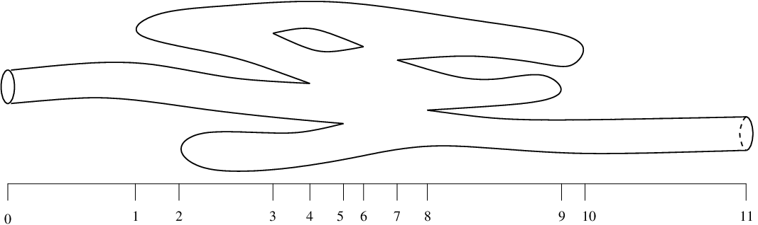
Let and let . For each , choose two link-grid diagrams and , such that: represents the link just before time ; represents the link just after time ; and can be obtained from by a link-grid move of Type , , or , depending on whether , , or , respectively. Observe that for each , the two link-grid diagrams and represent isotopic links; it is easy to see that while choosing and , we can ensure that the corresponding link components contain the same number of special -markings. Therefore, by Lemma 4.1, we can convert to by a sequence of link-grid moves of Types -. Putting everything together, we get the required sequence of link-grid moves that converts to . ∎
Proof of Theorem 3.4.
In order to prove this, we only need to show the following: if and are two tight link-grid diagrams representing knots and , respectively, and if there is a connected knot cobordism of genus from to , then .
Let us now assume that the cobordism from to has births, deaths and saddles. Theorem 4.2 tells us that there is a sequence of link-grid moves of Types - taking to , such that there are exactly link-grid moves of Type , link-grid moves of Type , link-grid moves of Type and link-grid moves of Type , and these link-grid moves happen in this order.
For link-grid moves of Types -, the associated maps on preserve Maslov gradings and are quasi-isomorphisms. For link-grid move , the map drops Maslov grading by , and is injective at the level of homology. The smallest Maslov grading also drops by , and by Theorem 3.1, the homology of in the smallest Maslov grading is . Therefore, the map on homology in the smallest Maslov grading is an isomorphism. Similarly, for link-grid move , the map increases Maslov grading by , and is surjective at the level of homology. However, the smallest Maslov grading also increases by ; therefore, the map on homology in the smallest Maslov grading is also an isomorphism. Thus, the composed maps from to preserves Maslov grading and is a quasi-isomorphism in the smallest Maslov grading. However, each of the link-grid diagrams and contains exactly one special -marking, so the smallest Maslov grading is the only Maslov grading in which the homology is supported. Therefore, the composed map is a quasi-isomorphism.
There are no Alexander grading shifts for link-grid moves , and , there is an Alexander grading shift of for link-grid moves and , and there is an Alexander grading shift of for link-grid moves and . Therefore, the net Alexander grading shift is . Therefore, for every , we have the following commuting square.
Substituting in the above commutative diagram, we see that the map is non-trivial; therefore, .
However, we can view the cobordism in reverse, i.e. we can run the movie backwards, to get a connected genus cobordism from to . That would show that . Combining the two inequalities, we get our desired result . ∎
5. Applications
Given any -grid diagram , define the special generator to be the generator whose coordinates lie at the top-left corners of the squares that contain the -markings. It is an easy computation to show that the Maslov grading of is always zero.
Let be the following index- -grid diagram: there is exactly one special -marking; the square containing lies immediately to the top-left of the square containing the special -marking; and for all , the square containing lies immediately to the top-left of the square containing . For this grid diagram, the special generator also has coordinates at the bottom-right corners of the squares that contain the -markings.
Lemma 5.1.
The -module generated by is a direct summand of .
Proof.
For any -grid diagram , the -module generated by is a quotient complex of . This is because any rectangle that joins some other generator to must pass through some -marking. However, rectangles are not allowed to pass through the special -markings, and whenever they pass through the normal -markings, they pick up a -power.
For the grid diagram , we would like to show that the -module generated by is also a subcomplex. Let be some generator that differs from in exactly two coordinates. There are exactly two embedded rectangles and , with boundary lying in , whose top-right and bottom-left corners are -coordinates, and whose top-left and bottom-right corners are -coordinates. It is clear that none of these rectangles contain any -markings or any -coordinates in their interiors. Therefore, , thereby concluding the proof. ∎
Lemma 5.2.
Let be an index- link-grid diagram that represents a knot , such that . Then .
Proof.
The link-grid diagram is a tight link-grid diagram representing , therefore, , which is the smallest , such that the map induced on homology from the inclusion is non-trivial. However, the homology of is one-dimensional, carried by the direct summand which is the -module generated by . Therefore . ∎

Let denote the -torus knot. We will represent by the following index- link-grid diagram : ; squares to the bottom-right of squares containing -markings also contain -markings; and the -marking in the horizontal annulus through the special -marking, lies squares to the right of the special -marking. The link-grid diagram is shown in Figure 5.1. To draw the torus knot that represents or to compute Alexander gradings of specific generators, we need to identify with a diagram on . For such identifications, we always assume that the special -marking lies in the bottom-right square.
Theorem 5.3.
There is an unknotting sequence for with crossing changes, and . Therefore, .
Proof.
Without loss of generality, let us assume that . After identifying with a picture on , let us consider the induced knot diagram for , cf. the first part of Figure 5.2. In this picture, there are crossings above the principal diagonal, and crossings below the principal diagonal, totalling to crossings (thus, this is actually a minimal crossing diagram for ).

Change the crossings above the principal diagonal. Figure 5.2 shows how we can isotope the resulting knot diagram to get the diagram that would be induced by . However, by induction, can be unknotted with crossing changes. Therefore, can be unknotted with crossing changes.
To compute , thanks to Lemma 5.2, we only need to compute the Alexander grading of the special generator . Towards this end, let us number the coordinates of from left to right as ; let us number the -markings from left to right as ; and let us number the special -marking as . Then,
Therefore, . Combining our results, we get , thus completing the proof. ∎
Acknowledgement
The work was done when the author was supported by the Clay Research Fellowship. He would like to thank John Baldwin, Robert Lipshitz, Peter Ozsváth and Zoltán Szabó for several helpful discussions. He would also like to thank the referee for many helpful comments.
References
- [BM94] Joan Birman and William Menasco, Special positions for essential tori in link complements, Topology 33 (1994), no. 3, 525–556.
- [Bru98] H. Brunn, Über verknotete Kurven, Verhandlungen des Internationalen Math Kongresses (Zurich 1897) (1898), 256–259.
- [Cro95] Peter Cromwell, Embedding knots and links in an open book I: Basic properties, Topology and its Applications 64 (1995), no. 1, 37–58.
- [Dyn06] Ivan Dynnikov, Arc-presentation of links: Monotonic simplification, Fundamenta Mathematicae 190 (2006), 29–76.
- [KM93] Peter Kronheimer and Tomasz Mrowka, Gauge theory for embedded surfaces I, Topology 32 (1993), no. 4, 773–826.
- [Lyo80] Herbert C. Lyon, Torus knots in the complement of links and surfaces, Michigan Math Journal 27 (1980), no. 1, 39–46.
- [Mat06] Hiroshi Matsuda, Links in an open book decomposition and in the standard contact structure, Proceedings of the American Mathematical Society 134 (2006), 3697–3702.
- [MOS09] Ciprian Manolescu, Peter Ozsváth, and Sucharit Sarkar, A combinatorial description of knot Floer homology, Annals of Mathematics 169 (2009), no. 2, 633–660.
- [MOSzT07] Ciprian Manolescu, Peter Ozsváth, Zoltán Szabó, and Dylan Thurston, On combinatorial link Floer homology, Geometry and Topology 11 (2007), 2339–2412.
- [Neu84] Lee Neuwirth, *-projections of knots, vol. Global Differential Geometry, Teubner-Texte zur Mathematik, no. 70, 1984.
- [Ni07] Yi Ni, Knot Floer homology detects fibred knots, Inventiones Mathematicae 170 (2007), no. 3, 577–608.
- [OSz03] Peter Ozsváth and Zoltán Szabó, Knot Floer homology and the four-ball genus, Geometry and Topology 7 (2003), 625–639.
- [OSz04a] by same author, Holomorphic disks and genus bounds, Geometry and Topology 8 (2004), 311–334.
- [OSz04b] by same author, Holomorphic disks and knot invariants, Advances in Mathematics 186 (2004), no. 1, 58–116.
- [OSz08] by same author, Holomorphic disks, link invariants and the multi-variable Alexander polynomial, Algebraic and Geometric Topology 8 (2008), 615–692.
- [OSzT08] Peter Ozsváth, Zoltán Szabó, and Dylan Thurston, Legendrian knots, transverse knots, and combinatorial link Floer homology, Geometry and Topology 12 (2008), 941–980.
- [Ras03] Jacob Rasmussen, Floer homology and knot complements, Ph.D. thesis, Harvard University, 2003.
- [Ras10] by same author, Khovanov homology and the slice genus, Inventiones Mathematicae 182 (2010), no. 2, 419–447.
- [Rud92] Lee Rudolph, Quasipositive annuli (constructions of quasipositive knots and links IV), Journal of Knot Theory and its Ramifications 4 (1992), 451–466.