Strong lensing of gravitational waves as seen by LISA

The space-based Laser Interferometer Space Antenna [1, LISA] is expected to observe gravitational waves (GWs) and open a new window for astronomy. Coalescencing massive black hole binaries (MBHBs) with total masses in the range $10^{3}$-$10^{7}~M_{\odot}$ out to $z\sim 10$-$15$ are expected to provide the loudest GW signals at LISA frequencies, $f\sim\mathrm{mHz}$ [2]. In the standard cold dark matter (CDM) hierarchical cosmology, MBHBs form in large number during the multiple mergers experienced by their host galaxies. LISA should detect from few to several hundreds coalescences per year. Within such promising premises we discuss a potential new chapter for LISA science: multiple imaging of distant sources by intervening lensing galaxies. Gravitational lensing statistics, in either quasar or radio-galaxy surveys, is usually considered on a sample of several thousands of sources. Due to the unprecedented high redshift of LISA sources, and the related very high optical depth for lensing, multiple events are possible even for hundreds of detections. Astrophysical and theoretical rewards might be valuable. $i)$ Lensing of GWs would be another impressive confirmation of the theory of general relativity. How GWs propagate near a massive body might shed light on competing theories of gravity. $ii)$ Constraints on cosmological parameters might be obtained in the range $z\mathrel{\lower 2.58334pt\hbox{$\mathrel{\mathop{\kern 0.0pt\scriptstyle\sim}\limits^{\textstyle>}}$}}10$. Measurements of time-delay, which can be accurately determined for transients [3], might be very useful. $iii)$ Lensing statistics might inform of the growth and structure of mass halos at $z\mathrel{\lower 2.58334pt\hbox{$\mathrel{\mathop{\kern 0.0pt\scriptstyle\sim}\limits^{\textstyle<}}$}}3$. The expected number of events strongly depends on the form and evolution of the galaxy number density. $iv)$ The magnification effect could help in finding electromagnetic counterparts and observing objects otherwise too distant or too faint.

Strong lensing by ground-based GW detectors was discussed in [4]. Here, we consider a lower frequency range where wave optics could play a role. Diffraction in lensing of GW is well understood [5] and is effective only for small lenses [6]. Our study on strong lensing is complementary to those on the weak lensing distortion of GW signals, which mainly focused on their use as standard sirens [7]. By default, we assume a flat $\Lambda$CDM model with $\Omega_{\mathrm{M}}=1-\Omega_{\Lambda}=0.3$, and $H_{0}=70~\mathrm{km~s}^{-1}\mathrm{Mpc}^{-1}$.

Lenses. Statistics of strong lenses is a well assessed astronomical tool [3]. Here, we mainly follow [8, 9]. The differential probability of a source to be lensed is

where $\sigma$ and $z_{\mathrm{d}}$ are the velocity dispersion and the redshift of the deflector, respectively, $s_{\mathrm{cr}}$ is the cross section and $dn/d\sigma$ is the differential lens number density. $dn/d\sigma$ can be modeled as a modified Schechter function [10]. This is accurate up to $z_{\mathrm{d}}\mathrel{\lower 2.58334pt\hbox{$\mathrel{\mathop{\kern 0.0pt\scriptstyle\sim}\limits^{\textstyle<}}$}}1$, where galaxies provide the bulk of the cross section for LISA sources. We took a conservative approach. Together with a constant comoving number density, we also considered a pessimistic scenario, i.e., an evolving case with a smaller number of lenses at high $z$ [11].

We account only for lensing by early type galaxies, modelled as singular isothermal spheres (SISs). Their Einstein radius is $R_{\mathrm{E}}=4\pi(\sigma/c)^{2}D_{\mathrm{d}}D_{\mathrm{ds}}/{D_{\mathrm{s}}}$; $D_{\mathrm{ds}}$, $D_{\mathrm{d}}$ and $D_{\mathrm{s}}$ are the angular diameter distances between the deflector and the source, and the observer and the lens or the source, respectively. Two images form at $x_{\pm}=y\pm 1$ if $y<1$, with flux magnification $\mu_{\pm}=(1/y)\pm 1$; $x$ and $y$ are the image and the source position normalized to the Einstein angular radius. The GW form is amplified by $A_{\pm}=\sqrt{\mu_{\pm}}$. $y$ can be measured through the ratio of the $A_{\pm}$. The delay between the arrival time of the images, $\Delta t=t_{-}-t_{+}$, is

For $\sigma\simeq 200~\mathrm{km~s}^{-1}$, $z_{\mathrm{d}}\simeq 5$ and $z_{\mathrm{s}}\simeq 10$, $\Delta t_{z}\simeq 100~\mathrm{days}$. LISA angular resolution is quite poor, $\sim 10^{\prime}$, but lenses are expected to be very massive and luminous. In case the deflector is located, one can precisely constrain the position of the source and try to detect it with follow-up observations. Combining measurements of $\Delta t$, $z_{\mathrm{d}}$ and $z_{\mathrm{s}}$, and $D_{\mathrm{s}}$ from the GW analysis might allow us to constrain $H_{0}$ and dark energy. A cosmographic approach independent of time-delay is based on lensing statistics [3].

The cross section for lensing is $s_{\mathrm{cr}}=\pi R_{\mathrm{E}}^{2}(y_{\mathrm{max}}^{2}-y_{\mathrm{min}}^{2})$, where $y_{\mathrm{min}}<y<y_{\mathrm{max}}$ is the allowed range to form detectable multiple images. $y_{\mathrm{max}}$ depends on the lens mass and redshift, the threshold signal to noise ratio ($\mathrm{SNR_{\mathrm{th}}}$), the unlensed amplitude ($\mathrm{SNR_{int}}$), see Eq. 3, the arrival time ($t_{+}$), and the total survey time ($T_{\mathrm{sur}}$, see Fig. 1). We considered $T_{\mathrm{sur}}=5~\mathrm{years}$. The emission frequency enters in $y_{\mathrm{min}}$, which excises the region near the central caustic where wave optics is effective. Geometric optics is valid for $y>y_{\mathrm{min}}$.

Lens discovery rates are affected by the ability to resolve multiple images [3]. Amplification has to push the signal above threshold, $A_{\pm}>\mathrm{SNR_{\mathrm{th}}^{\pm}}/\mathrm{SNR_{int}}$, which limits the source position to

according as the requirement is on the $+$ or the $-$ image, respectively. Multiple events are detectable if $y\leq y_{\mathrm{max}}^{-}$, which goes to 1 only for $\mathrm{SNR_{int}}\gg\mathrm{SNR_{\mathrm{th}}^{-}}$.

Due to the finite duration of the survey, statistics of transient phenomena involve some missing events due to time delay [3]. To observe both images, we require that $\Delta t<T_{\mathrm{sur}}-t_{+}$, which further constrains the source position. In Fig. 1, we plot $y_{\mathrm{max}}$ due to the finite observation time as a function of $z_{\mathrm{d}}$. This constraint plays a role only for very massive lenses, which are very rare, or for very late arrival times.

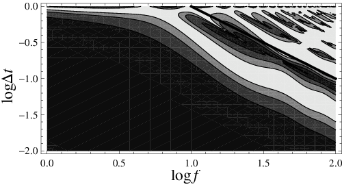
Wave-optics. Since we cannot observe multiple images when the interference pattern is pronounced, we have to discard configurations where wave effects are large [5]. Diffraction is negligible when the wavelength is much smaller than the gravitational radius of the lens, i.e., $\Delta t\gg f^{-1}$ [5]. Geometric optics is valid if the coherence time of the signal is much smaller than the time delay between images, $\Delta f\Delta t\gg 1$, where $\Delta f$ is either the bandwidth of the detector or the range in emission frequency. These conditions determine $y_{\mathrm{min}}$. The error in the estimated wave amplitude introduced by neglecting diffraction is displayed in Fig. 2, where we exploited the sum representation of the diffraction integral [5].

Two features determine the effective frequency for MBHBs. First, most of the signal is emitted near the coalescence time. Second, LISA sensitivity drops for $f\mathrel{\lower 2.58334pt\hbox{$\mathrel{\mathop{\kern 0.0pt\scriptstyle\sim}\limits^{\textstyle>}}$}}f_{\mathrm{ch}}=3\times 10^{-3}~\mathrm{Hz}$. The effective frequency is then the minimum between $f$ at coalescence and $f_{\mathrm{ch}}$. Since the final frequency is much larger than the initial one, the two conditions give very similar constraints. Apart from a very small region near the central caustic, see Fig. 3, wave effects are negligible. For a source $z_{\mathrm{s}}=6$ emitting at $f_{\mathrm{ch}}$ behind a massive lens ($\sigma\simeq 150~\mathrm{km/s}$, $z_{\mathrm{d}}=2$), $y_{\mathrm{min}}\simeq 10^{-2}$.

Optical depth. The lensing probability for a source is the total optical depth $\tau$, obtained by integrating Eq. (1); it is plotted in Fig. 4 as a function of $z_{\mathrm{s}}$. In our standard case, $\Omega_{\mathrm{M}}=0.3$, the comoving $dn/d\sigma$ is constant and $\mathrm{SNR_{\mathrm{th}}^{\pm}}=8$ is the detection threshold. The more effective constraint on the cross section is the requirement of a loud enough second image. If we either lower $\mathrm{SNR_{\mathrm{th}}^{-}}$ or consider intrinsically brighter signals, $\tau$ dramatically increases. $\tau$ is very sensitive to the value of $\Lambda$ and goes down for a smaller number of lenses at high $z$.

Probabilities are quite large for a range of BH binaries with masses ($10^{4}$-$10^{7}M_{\odot}$) and redshifts ($z\mathrel{\lower 2.58334pt\hbox{$\mathrel{\mathop{\kern 0.0pt\scriptstyle\sim}\limits^{\textstyle<}}$}}15$) of astrophysical relevance in the LISA window, see Fig. 5. $\tau$ is plotted in the standard case as a function of $z$ and the main BH mass, $M_{1}$, for two different mass ratios. The $\mathrm{SNR_{int}}$ of a given merger was computed according to [2]. Given $M_{1}$, the larger the mass ratio, the larger $\tau$.

LISA sources. To estimate the lensing probabilities we need plausible merger rates. We adopt MBH assembly histories created via dedicated Monte Carlo merger tree simulations framed in the hierarchical paradigm [12]. Either first seed BHs are light, $M\gtrsim 100M_{\odot}$, being the remnant of the first POPIII star explosions [13] or already quite heavy ($M\gtrsim 10^{4}M_{\odot}$) seeds form by direct collapse of proto-galactic discs [14], or through efficient accretion onto a “quasi star” forming in dense disks prone to bars-within-bars instabilities [15]. The first two models we analyzed (Light and Heavy models, LE and SE in [16], respectively) have been adopted as a benchmark for model comparison by the LISA parameter estimation taskforce. Furthermore, we considered a pair of “hybrid” models where the two formation processes coexist and the seed mass spectrum spans the range $10^{2}$-$10^{5}M_{\odot}$ [17]. The two hybrid models have somewhat different formation efficiencies, which are set by the maximum spin parameter $\lambda_{\mathrm{Thr}}$ of the halo that allows an efficient inflow of gas in the nuclear region. We considered a conservative version ($\lambda_{\mathrm{Thr}}=0.01$, HybridI) and a more optimistic one ($\lambda_{\mathrm{Thr}}=0.02$, HybridII).

All models have been extensively tested against observational constraints, such as the present day mass density of nuclear MBHs, the optical and X-ray luminosity functions of quasars and the unresolved X-ray background [12]. Light, Heavy and HybridI models are on the conservative side, while HybridII is more optimistic. LISA source redshifts are much higher than usual, see Table 1, and allow to investigate the Universe to very large distances. By comparison, radio-sources in the CLASS survey had $\bar{z}_{\mathrm{s}}=1.4\pm 0.7$ [3].

Expected events. The mean number of lenses expected to be observed, $\langle N\rangle$, is given by the sum of the optical depths of all the sources. We simulated the intrinsic properties instead of the observed distribution of amplitudes so that we did not have to correct for any magnification bias [3]. Results are listed in Table 1. The Poissonian probability for multiple events is plotted in Fig. 6. Chances are fairly large for all the build-up scenarios. Wave effects are negligible: in the geometric optics limit ($y_{\mathrm{min}}=0$), $\tau_{\mathrm{tot}}$ increases by $\mathrel{\lower 2.58334pt\hbox{$\mathrel{\mathop{\kern 0.0pt\scriptstyle\sim}\limits^{\textstyle<}}$}}0.01\%$.

The bulk of the total cross section is due to high $\mathrm{SNR_{int}}$ events. In the Light scenario, the fraction of events ($\sim 54\%$) intrinsically below threshold contributes only $\mathrel{\lower 2.58334pt\hbox{$\mathrel{\mathop{\kern 0.0pt\scriptstyle\sim}\limits^{\textstyle<}}$}}8\%$ of $\tau_{\mathrm{tot}}$. Due to the many events with very high $\mathrm{SNR_{int}}$, results for the Heavy case are not affected at all by lowering $\mathrm{SNR_{\mathrm{th}}^{-}}$, whereas probabilities increase significantly in the Light and HybridI cases. LISA should detect independently two above threshold signals in the same position in order to claim lensing. Any dedicated pipeline for detection of double peaked events might strong enhance lensing detection.

A larger, but still compatible with observations, $\Lambda$ strongly increases the probabilities. New merger trees should be generated, but to stress the role played by a larger $\Lambda$ we focused on the variation of $\tau$. Reducing the number of lenses at high $z$ has an opposite effect but chances are still sizable.

Lensing amplification can make some intrinsically too faint mergers luminous enough to be detected. If we are not interested in the second image, $y_{\mathrm{max}}$ can be larger than one and is determined only by the flux condition on the $+$ image. In the Light (HybridI) model, nearly $3(2)\%$ of the otherwise undetected events, $\mathrel{\lower 2.58334pt\hbox{$\mathrel{\mathop{\kern 0.0pt\scriptstyle\sim}\limits^{\textstyle>}}$}}1$ event per year, may become loud enough to be seen. In the HybridII scenario, $8\pm 3$ additional events per 5 years are expected.

We provided one of the first attempts at formalizing lensing statistics in presence of wave-effects. Our assumptions were conservative: a 5 years mission; high detection thresholds; not so optimistic formation scenarios; no account of lensing by late-type galaxies, whose distribution is poorly known but contribute $\mathrel{\lower 2.58334pt\hbox{$\mathrel{\mathop{\kern 0.0pt\scriptstyle\sim}\limits^{\textstyle<}}$}}30\%$ of $\tau_{\mathrm{tot}}$ [3]. Probabilities to observe multiple events were anyway sizable, from $\mathrel{\lower 2.58334pt\hbox{$\mathrel{\mathop{\kern 0.0pt\scriptstyle\sim}\limits^{\textstyle<}}$}}20$ to $\mathrel{\lower 2.58334pt\hbox{$\mathrel{\mathop{\kern 0.0pt\scriptstyle\sim}\limits^{\textstyle<}}$}}100\%$. Lensing statistics depend on the cosmological parameters, suggesting new potential tools for cosmography with LISA. In case of optical identification of lenses, additional measurements of time-delay might help to constrain $H_{0}$ and dark energy. $\tau$ is very sensitive to $dn/d\sigma$ too, which might help to understand evolution of early-type galaxies up to high redshifts.

The main unsureness in our forecast is due to the uncertain build-up process. Tight predictions need knowledge of galaxy evolution at high $z$, one of the main LISA goals. To establish that lensing probabilities for LISA might be significant and to point to the relative rewards, it was enough to consider a broad range of formation scenarios without trying to maximize $\tau_{\mathrm{tot}}$. Hopefully, LISA lensing might help to constrain the formation history.

Apart from astronomical applications, the detection of even a single GW lensing event would provide unique information on competing theories of gravity by allowing to test velocity and propagation of gravity. Up to now, GWs are still missing on an experimental ground. Their mere detection by LISA would be a success. Serendipitous GW lensing might be an extremely beneficial bonus.

References

- [1] K. Danzmann and the LISA study team, Classical Quantum Gravity 13, A247 (1996).
- [2] S. A. Hughes, Mon. Not. R. Astron. Soc. 331, 805 (2002); A. Klein, P. Jetzer, and M. Sereno, Phys. Rev. D 80, 064027 (2009). A. Sesana, et al., Astrophys. J. 623, 23 (2005); A. Sesana, M. Volonteri, and F. Haardt, Mon. Not. R. Astron. Soc. 377, 1711 (2007).
- [3] E. L. Turner, Astroph. J. Lett. 365, L43 (1990); C. S. Kochanek, Astrophys. J. 419, 12 (1993). K.-H. Chae, Mon. Not. R. Astron. Soc. 346, 746 (2003); M. Oguri, Y. Suto, and E. L. Turner, Astrophys. J. 583, 584 (2003).
- [4] Y. Wang, A. Stebbins, and E. L. Turner, Physical Rev. Lett. 77, 2875 (1996).
- [5] P. Schneider, J. Ehlers, and E. E. Falco, Gravitational Lenses (Springer-Verlag Berlin, 1992); T. T. Nakamura and S. Deguchi, Prog. Theor. Phys. Suppl. 133, 137 (1999); R. Takahashi and T. Nakamura, Astrophys. J. 595, 1039 (2003). N. Matsunaga and K. Yamamoto, J. Cosmol. Astropart. Phys. 1, 23 (2006).
- [6] C. Yoo, et al., Astrophys. J. 655, 691 (2007); N. Seto, Phys. Rev. D 80, 103001 (2009);
- [7] B. F. Schutz, Nature (London) 323, 310 (1986); C. Shapiro, et al., Mon. Not. R. Astron. Soc. 404, 858 (2010).
- [8] M. Sereno, Mon. Not. R. Astron. Soc. 356, 937 (2005).
- [9] Z. Zhu and M. Sereno, Astron. Astroph. 487, 831 (2008).
- [10] R. K. Sheth, et al., Astrophys. J. 594, 225 (2003); Y. Choi, C. Park, and M. S. Vogeley, Astrophys. J. 658, 884 (2007).
- [11] K. Chae, Astroph. J. Lett. 658, L71 (2007).
- [12] M. Volonteri, F. Haardt, and P. Madau, Astrophys. J. 582, 559 (2003); G. Kauffmann and M. Haehnelt, Mon. Not. R. Astron. Soc. 311, 576 (2000); R. K. Malbon, et al., Mon. Not. R. Astron. Soc. 382, 1394 (2007). M. Volonteri, G. Lodato and P. Natarajan, Mon. Not. R. Astron. Soc. 383, 1079 (2008).
- [13] P. Madau and M. J. Rees, Astroph. J. Lett. 551, L27 (2001).
- [14] S. M. Koushiappas, J. S. Bullock, and A. Dekel, Mon. Not. R. Astron. Soc. 354, 292 (2004); G. Lodato and P. Natarajan, Mon. Not. R. Astron. Soc. 371, 1813 (2006).
- [15] M. C. Begelman, M. Volonteri, and M. J. Rees, Mon. Not. R. Astron. Soc. 370, 289 (2006).
- [16] K. G. Arun, et al., Classical Quantum Gravity 26, 094027 (2009).
- [17] M. Volonteri and M. C. Begelman, ArXiv:1003.5220.