跳到论文正文
W Papers独立论文阅读器 arXiv:1011.5104 论文正文 计算阅读时间 · 0%
引用这篇论文根据当前论文元数据生成,正式投稿前建议核对。


License: arXiv.org perpetual non-exclusive license
arXiv:1011.5104v3 [math.PR] 06 Dec 2010

On the superposition of heterogeneous traffic
at large time scales

Luis López-Oliveros Address: Luis López-Oliveros
Department of Statistical Science
Cornell University
Ithaca, NY 14853
Email address: ll278@cornell.edu
and Sidney I. Resnick Address: Prof. Sidney Resnick
School of Operations Research and Information Engineering
Cornell University
Ithaca, NY 14853
Email address: sir1@cornell.edu
Abstract.

Various empirical and theoretical studies indicate that cumulative network traffic is a Gaussian process. However, depending on whether the intensity at which sessions are initiated is large or small relative to the session duration tail, Mikosch et al (2002) and Kaj and Taqqu (2008) have shown that traffic at large time scales can be approximated by either fractional Brownian motion (fBm) or stable Lévy motion. We study distributional properties of cumulative traffic that consists of a finite number of independent streams and give an explanation of why Gaussian examples abound in practice but not stable Lévy motion. We offer an explanation of how much vertical aggregation is needed for the Gaussian approximation to hold. Our results are expressed as limit theorems for a sequence of cumulative traffic processes whose session initiation intensities satisfy growth rates similar to those used in Mikosch et al (2002).

1. Introduction

Collection of data network measurements often uses an algorithm for clustering packets with the same source and destination IP addresses. Various criteria for grouping packets yield different entities, e.g. connections, flows (or unidirectional connections), end-to-end streams, etc. (See e.g. Sarvotham et al, 2005, Section 4). These high-order constructs of packet clusters are sometimes termed sessions. For now, think of a session as a user downloading a file, streaming media, or accessing websites. For each session, summary measurements are computed for the size (the number of bytes transmitted in a session), the duration of the session and the average transfer rate. Data sets of these summaries show some distinctive properties, such as heavy tails for session size and duration (Arlittson and Williamson, 1996; Crovella and Bestavros, 1997; Willinger et al, 1998) and sometimes rate (Maulik et al, 2002; Resnick, 2003).

Typically, a time resolution or granularity is selected or imposed. Typical resolutions are 1, 10 or 100 milliseconds, 1 second, 1 minute, 1 hour, etc. Once a resolution is fixed, the number of bytes or number of packets per unit time can be recorded and cumulative network loads over stationary time intervals computed. These cumulative loads have been studied from empirical and theoretical perspectives with the objectives of satisfying performance criterion and offering adequate bandwidth provisioning (van de Meent and Mandjes, 2005) or predicting properties of congestion events (Jin et al, 2007).

Conventional wisdom based on empirical studies claims that a heavily loaded network link subject to aggregation over many users should see Gaussian traffic. This wisdom is considered a network invariant. Influential examples based on the Bellcore measurements (Leland et al, 1994) suggest that horizontal aggregation, that is, working with a single on/off stream at sufficiently large time scale justifies Gaussian modeling. See also Kurtz (1996) and Willinger et al (1997).

However, mathematically it is known that with heavy tailed session durations, cumulative load at large time scales can be approximated by either fractional Brownian motion (fBm) or stable Lévy motion, depending on whether the intensity at which sessions are initiated is large or small relative to the size of the duration tails. See Mikosch et al (2002); Kaj and Taqqu (2008); Taqqu et al (1997). The stable approximation has not been observed empirically (Guerin et al, 2003) and use of Gaussian cumulative loads has become dominant (Kilpi and Norros, 2002; Sarvotham et al, 2002; Jain and Dovrolis, 2005).

But why should traffic be Gaussian? According to the empirical study van de Meent et al (2006), in addition to horizontal aggregation, the superposition of independent traffic streams, that is, vertical aggregation, can justify a Gaussian model and, in fact, the number of traffic streams need not be large to make cumulative loads approximately Gaussian.

In this paper we

  • •

    study the distribution of the cumulative load in the presence of a finite number of independent traffic streams;

  • •

    give an explanation for why Gaussian examples abound in practice but not stable ones;

  • •

    answer how much vertical aggregation is needed to justify the use of fBm.

Our findings suggest that cumulative load for aggregate traffic can be approximated by fBm at large time scales provided the initiation intensity of at least one of the traffic components is large. Network traffic in the wild has several distinct constituents and we claim that in practice there is one or more components with dominant large initiation intensities. For example, this should be the case with web traffic using port 80 and this suggests why Gaussian traffic should be pervasive (van de Meent et al, 2006).

Before discussing mathematical details, we illustrate the phenomena of interest with a motivating example of a network trace captured at Cornell University main campus servers during 55 days between November 2, 2009, and January 15, 2010. Cornell’s data set is a collection of netflow records, where all non-IP traffic has been discarded and only TCP and UPD traffic is present in the trace. A netflow is a collection of packets with the same source and destination IP addresses, source and destination ports, protocol, ingress interface and IP type of service (Cisco Systems, Inc., 2007). In our data, TCP traffic accounts for nearly 90% of the bytes, and over 80% of the total number of netflows, mostly port 80 (http traffic) netflows. We have taken the part of the trace corresponding to both outgoing and incoming traffic between 1 and 5 p.m. local time, adding up to 220 hours of traffic. The anonymization procedure used on the data obliterated the distinction between outgoing and incoming flows.

We analyze the distribution of A(T​C​P)A^{(TCP)} and A(U​D​P)A^{(UDP)}, namely the cumulative load generated by TCP and UDP bytes, respectively. For this purpose, we separate the trace into TCP and UDP netflows and for k=1,…,220k=1,\ldots,220 we count

Ak(T​C​P)\displaystyle A_{k}^{(TCP)} :=total number of TCP bytes captured in the kth hour,\displaystyle:=\textrm{total number of TCP bytes captured in the $k$th hour},
Ak(U​D​P)\displaystyle A_{k}^{(UDP)} :=total number of UDP bytes captured in the kth hour.\displaystyle:=\textrm{total number of UDP bytes captured in the $k$th hour}.

Due to the dates and times of collection, these counts exhibit both a trend and a daily seasonality. Here we detrend and remove daily seasonality (see e.g. Brockwell and Davis, 1991, Section 1.4), but our conclusions are the same without this massage.

Figure 1 shows Gaussian QQ plots for A(T​C​P)A^{(TCP)} (left) and A(U​D​P)A^{(UDP)} (right). A straight line fit is evident for the TCP cumulative input. However, the UDP counterpart shows a significant departure from the straight line. Using the pp-values of the Anderson-Darling two-sided test also shows no evidence against the normality of A(T​C​P)A^{(TCP)} (p=0.1369p=0.1369), but strong evidence against a Gaussian model for A(U​D​P)A^{(UDP)} (p=9.8×10⁻¹⁶p=9.8\times 10^{-16}).

Refer to caption
Figure 1. Normal QQ plots of cumulative inputs. Left: TCP traffic. Right: UDP traffic

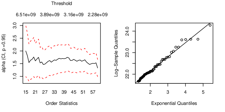
We also check whether A(U​D​P)A^{(UDP)} is a heavy-tailed random variable, in the sense of its distribution tail being regularly varying with tail index α\alpha (de Haan and Ferreira, 2006; Resnick, 2007). For instance, Figure 2 left shows a stable regime in the Hill plot of α\alpha (Hill, 1975; de Haan and Resnick, 1998; Resnick, 2007, for Hill plots, see e.g.). Additionally, in Figure 2 right we present the exponential QQ plot of log⁡(A(U​D​P))\log(A^{(UDP)}) with a straight line fit through the biggest 55 observations. This shows no evidence against approximating the distribution of thresholded values of A(U​D​P)A^{(UDP)} by a Pareto (Recall that the logarithm of Pareto random variable is exponential; see, for example, Mc Neil et al (2005); Resnick (2007); Coles (2001).)
Refer to caption
Figure 2. Plots for the UDP cumulative input. Left: Hill plot of tail index with 95% confidence interval. Right: Exponential QQ plot of the log data.

If we consider the aggregated cumulative load, A(T​C​P)+A(U​D​P)A^{(TCP)}+A^{(UDP)}, the normal QQ plot in Figure 3 exhibits a straight line fit and the Anderson-Darling test p−p-value is 0.21170.2117, showing no evidence to reject normality. Without accounting for centering and scaling, this result is rather counterintuitive due to the nature of the individual tails of A(T​C​P)A^{(TCP)} and A(U​D​P)A^{(UDP)}.

Refer to caption
Figure 3. Normal QQ plot of the aggregated cumulative input.

Our explanation to the above phenomenon starts by modeling the quantity of data in windows of length TT in Section 2. Analogously to the slow and fast growths of Mikosch et al (2002), we define two different scenarios for the aggregated traffic. A third scenario is defined similarly to the boundary case considered in Kaj and Taqqu (2008). In Section 3 we obtain approximations and provide clarification of the asymptotic behavior at large time scales. We let T→∞T\to\infty and see what limits exist for the aggregated cumulative load. In Section 4 we study extensions to our model and finally Section 5 contains some technical results used to prove our main theorems.

1.1. Notation

In order to simplify the later presentation, we introduce and collect some notation. References are provided for further reading.

F¯\bar{F} The right tail of the distribution function FF, i.e. F¯=1−F\bar{F}=1-F.
F←F^{\leftarrow} The left continuous inverse of the distribution function FF,
i.e. F←​(y)=inf{x:F⁡(x)≥y}F^{\leftarrow}(y)=\inf\{x:F(x)\geq y\}.
f1∼f2f_{1}\sim f_{2} limx→∞f1​(x)/f2​(x)=1\lim_{x\to\infty}f_{1}(x)/f_{2}(x)=1.
→f​i​d​i\xrightarrow{fidi} Convergence of finite dimensional distributions.
→𝑣\xrightarrow{v} Vague convergence of measures. See e.g. Kallenberg (1984); Resnick (1987).
M+(0,∞]M_{+}(0,\infty] The space of nonnegative Radon measures on (0,∞](0,\infty].
R​VγRV_{\gamma} The class of regularly varying functions with index γ\gamma.
See e.g. Bingham et al (1987); de Haan and Ferreira (2006); Resnick (1986).
ξ=ℙ​ℝ​𝕄​(E​ξ)\xi=\mathbb{PRM}(E\xi) A Poisson random measure ξ\xi with mean measure E​ξE\xi.
𝜉∘{\mathrel{\mathop{\kern 0.0pt\xi}\limits^{{}_{\circ}}}} A compensated Poisson random measure with mean measure E​ξE\xi, i.e. 𝜉∘=ξ−Eξ{\mathrel{\mathop{\kern 0.0pt\xi}\limits^{{}_{\circ}}}}=\xi-E\xi.
Nγ,hδ∞N^{\infty}_{\gamma,h_{\delta}} Nγ,hδ∞=ℙ​ℝ​𝕄​(d​s⋅γ​u−(γ+1)​d​u⋅hδ​(d​r))N^{\infty}_{\gamma,h_{\delta}}=\mathbb{PRM}(ds\cdot\gamma u^{-(\gamma+1)}du\cdot h_{\delta}(dr)) on ℝ×(0,∞)2\mathbb{R}\times(0,\infty)^{2}, where hδh_{\delta} is a measure on (0,∞)(0,\infty)
such that hδ[⋅,∞)∈RV−δh_{\delta}[\cdot,\infty)\in RV_{-\delta}. If hδ​(d​r)=δ​r−(δ+1)​d​rh_{\delta}(dr)=\delta r^{-(\delta+1)}dr, we may simply write Nγ,δ∞N^{\infty}_{\gamma,\delta}.
Nγ,δ∞N^{\infty}_{\gamma,\delta} Nγ,δ∞=ℙ​ℝ​𝕄​(d​s⋅γ​u−(γ+1)​d​u⋅δ​r−(δ+1)​d​r)N^{\infty}_{\gamma,\delta}=\mathbb{PRM}(ds\cdot\gamma u^{-(\gamma+1)}du\cdot\delta r^{-(\delta+1)}dr) on ℝ×(0,∞)2\mathbb{R}\times(0,\infty)^{2}.
Mγ,m​(d​v)M_{\gamma,m}(dv) A γ−\gamma-stable random measure with control measure m⁡(d​v)m(dv) and stable index 1<γ<21<\gamma<2.
For ξ=ℙ​ℝ​𝕄​(m⁡(d​v)​w−(ρ+1)​d​w)\xi=\mathbb{PRM}(m(dv)w^{-(\rho+1)}dw), we can write
Mγ,m(A)=d((−cosπ​γ2)2​Γ​(2−γ)γ⁡(γ−1))−1/γ∫A∫w=0∞w𝜉∘(dv,dw)M_{\gamma,m}(A)\stackrel{{\scriptstyle d}}{{=}}\left(\left(-\cos\frac{\pi\gamma}{2}\right)\frac{2\Gamma(2-\gamma)}{\gamma(\gamma-1)}\right)^{-1/\gamma}\int_{A}\int_{w=0}^{\infty}w{\mathrel{\mathop{\kern 0.0pt\xi}\limits^{{}_{\circ}}}}(dv,dw).
See e.g. Samorodnitsky and Taqqu (1994, Chapter 3).
Λγ​(⋅)\Lambda_{\gamma}(\cdot) A γ−\gamma-stable Lévy motion totally skewed to the right with stable index 1<γ<21<\gamma<2.
In general, we can write Λγ(t)=d((−cosπ​γ2)2​Γ​(2−γ)γ⁡(γ−1))1/γ∫0∞1{0<v<t}Mρ,m(dv)\Lambda_{\gamma}(t)\stackrel{{\scriptstyle d}}{{=}}\left(\left(-\cos\frac{\pi\gamma}{2}\right)\frac{2\Gamma(2-\gamma)}{\gamma(\gamma-1)}\right)^{1/\gamma}\int_{0}^{\infty}1_{\{0<v<t\}}M_{\rho,m}(dv).
See e.g. Samorodnitsky and Taqqu (1994, Chapter 3).
BH​(⋅)B_{H}(\cdot) The standard fractional Brownian motion with Hurst exponent HH.

2. Model Description and Basic Assumptions

Consider a network that has an infinite number of nodes. At certain times, a node begins a transmission session at a random rate that is fixed throughout the session. Suppose network traffic consists of pp distinct types which we call streams. In practice, such a division of network traffic arises naturally; e.g. traffic can be segmented by application type (web, email, streaming media, file-sharing applications, etc.), by protocol (TCP, UDP, IMTP, etc.), and even by users. We suppose the pp streams are independent and that each follows an M/G/∞M/G/\infty input model. The overall load is obtained by aggregating over the pp streams. Thus, the basic assumptions are as follows:

  • •

    Sessions corresponding to the jjth stream are initiated at homogenous Poisson time points {Γk(j),−∞<k<∞}\{\Gamma_{k}^{(j)},-\infty<k<\infty\} with arrival intensity λ(j)>0\lambda^{(j)}>0. These points are labeled so that Γ0(j)<0<Γ1(j)\Gamma_{0}^{(j)}<0<\Gamma_{1}^{(j)} whence {−Γ0(j),Γ1(j),(Γk+1(j)−Γk(j),k≠0)}\{-\Gamma_{0}^{(j)},\Gamma_{1}^{(j)},(\Gamma_{k+1}^{(j)}-\Gamma_{k}^{(j)},k\not=0)\} are iid exponential with parameter λ(j)\lambda^{(j)}. Thus, we have:

    ∑kϵΓk(j)=ℙ​ℝ​𝕄​(λ(j)​d​s).\sum_{k}\epsilon_{\Gamma_{k}^{(j)}}=\mathbb{PRM}(\lambda^{(j)}ds).

    We assume that these ℙ​ℝ​𝕄\mathbb{PRM}s are independent.

  • •

    All the sessions in the network transmit data at positive random rates that are iid with common distribution FRF_{R}. Let {Rk(j)}\{R_{k}^{(j)}\} be the rate of the kkth session of the jjth stream. Assume that either F¯R∈R​V−αR,1<αR<2\bar{F}_{R}\in RV_{-\alpha_{R}},1<\alpha_{R}<2, or E⁡[(R1(1))2]<∞E[(R_{1}^{(1)})^{2}]<\infty. In either case, define μR:=E​R1(1)\mu_{R}:=ER_{1}^{(1)}.

  • •

    Sessions in the jjth stream have positive durations {Dk(j)}\{D_{k}^{(j)}\}, j=1,…,p,j=1,\ldots,p, that are iid FD(j)F_{D}^{(j)}, with F¯D(j)∈R​V−αD(j)\bar{F}_{D}^{(j)}\in RV_{-\alpha_{D}^{(j)}}, 1<αD(j)<21<\alpha_{D}^{(j)}<2, and μD(j):=E​D1(j)\mu_{D}^{(j)}:={ED^{(j)}_{1}}. In general, not all the αD(j)\alpha_{D}^{(j)}s are equal.

  • •

    We also assume mutually independent durations across streams, and that durations and rates are independent.

There is empirical evidence justifying the choices of αD(j)\alpha_{D}^{(j)}s and αR\alpha_{R}: See e.g. Cunha et al (1995); Willinger et al (1995); Leland et al (1994); Resnick (2003); López-Oliveros and Resnick (2009). For now, we adopt a network-centric approach by assuming the rate of communication entirely depends on the state and speed of the network. Studies supporting this assumption include Shakkottai et al (2005) and Kortebi et al (2005).

We will need

λ=∑j=1pλ(j),\lambda=\sum_{j=1}^{p}\lambda^{(j)}, (2.1)
FD:=∑j=1p(λ(j)/λ)​FD(j),F_{D}:=\sum_{j=1}^{p}(\lambda^{(j)}/\lambda)F_{D}^{(j)}, (2.2)

and the quantile functions

bD(j)​(t)\displaystyle b_{D}^{(j)}(t) =(1/F¯D(j))←​(t)=(FD(j))←​(1−1/t),\displaystyle=(1/\bar{F}_{D}^{(j)})^{\leftarrow}(t)=(F_{D}^{(j)})^{\leftarrow}(1-1/t), (2.3)
bD​(t)\displaystyle b_{D}(t) =(1/F¯D)←​(t)=FD←​(1−1/t),\displaystyle=(1/\bar{F}_{D})^{\leftarrow}(t)=F_{D}^{\leftarrow}(1-1/t), (2.4)
bR​(t)\displaystyle b_{R}(t) =(1/F¯R)←​(t)=FR←​(1−1/t).\displaystyle=(1/\bar{F}_{R})^{\leftarrow}(t)=F_{R}^{\leftarrow}(1-1/t). (2.5)

Notice that FDF_{D} is the mixture model of the durations of the pp streams, with weights λ(j)/λ\lambda^{(j)}/\lambda, j=1,…,pj=1,\ldots,p. In fact, FDF_{D} is the distribution of the duration of the sessions of the aggregated stream, and λ(j)/λ\lambda^{(j)}/\lambda is the proportion of the traffic that consists of sessions from the jjth stream. We return to this interpretation later.

Now consider (s,u,r)(s,u,r) as a generic Poisson point representing a session that starts at time ss, has duration uu and rate rr. By augmentation, the counting function of the session descriptors (Γk(j),Dk(j),Rk(j))(\Gamma_{k}^{(j)},D_{k}^{(j)},R_{k}^{(j)}) of the jjth stream on ℝ×[0,∞)2\mathbb{R}\times[0,\infty)^{2} is

N(j):=∑kϵ(Γk(j),Dk(j),Rk(j))=ℙℝ𝕄(λ(j)dsFD(j)(du)FR(dr)),j=1,…,p.N^{(j)}:=\sum_{k}\epsilon_{(\Gamma_{k}^{(j)},D_{k}^{(j)},R_{k}^{(j)})}=\mathbb{PRM}(\lambda^{(j)}dsF_{D}^{(j)}(du)F_{R}(dr)),\quad j=1,\ldots,p. (2.6)

By independence, the counting function of the session descriptors of the aggregated stream is

N:=∑j=1pN(j)\displaystyle N:=\sum_{j=1}^{p}{N^{(j)}} =ℙ​ℝ​𝕄​(λ​d​s​∑j=1p(λ(j)/λ)​FD(j)​(d​u)​FR​(d​r))\displaystyle=\mathbb{PRM}\left(\lambda ds\sum_{j=1}^{p}(\lambda^{(j)}/\lambda)F_{D}^{(j)}(du)F_{R}(dr)\right)
=ℙ​ℝ​𝕄​(λ​d​s​FD​(d​u)​FR​(d​r)).\displaystyle=\mathbb{PRM}(\lambda dsF_{D}(du)F_{R}(dr)). (2.7)

Thus, the mean measures of the N(j)N^{(j)} and NN are given by

E​N(j)​(d​s,d​u,d​r)\displaystyle EN^{(j)}(ds,du,dr) :=λ(j)dsFD(j)(du)FR(dr),j=1,…,p,\displaystyle:=\lambda^{(j)}dsF_{D}^{(j)}(du)F_{R}(dr),\quad j=1,\ldots,p,
E​N​(d​s,d​u,d​r)\displaystyle EN(ds,du,dr) :=λ​d​s​FD​(d​u)​FR​(d​r).\displaystyle:=\lambda dsF_{D}(du)F_{R}(dr).

In addition, let

Lt​(s,u)=|[0,t]∩[s,s+u]|=∫0t1[s,s+u]​(y)​𝑑y=∫0u1[0,t]​(y+s)​𝑑y,L_{t}(s,u)=\left|[0,t]\cap[s,s+u]\right|=\int_{0}^{t}1_{[s,s+u]}(y)dy=\int_{0}^{u}1_{[0,t]}(y+s)dy, (2.8)

be the length of the subinterval of [0,t][0,t] during which the session (s,u,r)(s,u,r) transmits data. In Lemma 5.4, we summarize several required properties of Lt​(s,u)L_{t}(s,u).

For each jj, define

A(j)​(t)\displaystyle A^{(j)}(t) :=cumulative input in [0,t] from the jth stream\displaystyle:=\textrm{cumulative input {in $[0,t]$ from} the $j$th stream}
=∫−∞∞∫0∞∫0∞r​Lt​(s,u)​N(j)​(𝑑s,𝑑u,𝑑r),\displaystyle=\int_{-\infty}^{\infty}\int_{0}^{\infty}\int_{0}^{\infty}rL_{t}(s,u)N^{(j)}(ds,du,dr), (2.9)
and similarly
A⁡(t)\displaystyle A(t) :=cumulative input in [0,t] from the aggregated stream\displaystyle:=\textrm{cumulative input {in $[0,t]$} from the aggregated stream}
=∫−∞∞∫0∞∫0∞r​Lt​(s,u)​N​(𝑑s,𝑑u,𝑑r).\displaystyle=\int_{-\infty}^{\infty}\int_{0}^{\infty}\int_{0}^{\infty}rL_{t}(s,u)N(ds,du,dr). (2.10)

(Kaj and Taqqu (2008) showed that these integrals are well defined using Campbell’s theorem (Kingman, 1993, Section 3.2).) Also,

E​A(j)​(t)=λ(j)​μD(j)​μR​t,E​A​(t)=∑j=1pλ(j)​μD(j)​μR​t=λ​μD​μR​t,EA^{(j)}(t)=\lambda^{(j)}\mu_{D}^{(j)}\mu_{R}t,\quad EA(t)=\sum_{j=1}^{p}\lambda^{(j)}\mu_{D}^{(j)}\mu_{R}t=\lambda\mu_{D}\mu_{R}t,

where

μD:=∑j=1p(λ(j)/λ)​μD(j)\mu_{D}:=\sum_{j=1}^{p}(\lambda^{(j)}/\lambda)\mu_{D}^{(j)} (2.11)

is the mean of the mixture model of the durations of the different streams.

Observe that we can write the cumulative inputs as linear drift plus compensated random Poisson fluctuation as follows:

A(j)​(t)\displaystyle A^{(j)}(t) :=λ(j)μD(j)μRt+∫−∞∞∫0∞∫0∞rLt(s,u)𝑁∘(j)(ds,du,dr),\displaystyle:=\lambda^{(j)}\mu_{D}^{(j)}\mu_{R}t+\int_{-\infty}^{\infty}\int_{0}^{\infty}\int_{0}^{\infty}rL_{t}(s,u){\mathrel{\mathop{\kern 0.0ptN}\limits^{{}_{\circ}}}}^{(j)}(ds,du,dr), (2.12)
A⁡(t)\displaystyle A(t) :=λ​μD​μR​t+∫−∞∞∫0∞∫0∞r​Lt​(s,u)𝑁∘(𝑑s,𝑑u,𝑑r).\displaystyle:=\lambda\mu_{D}\mu_{R}t+\int_{-\infty}^{\infty}\int_{0}^{\infty}\int_{0}^{\infty}rL_{t}(s,u){\mathrel{\mathop{\kern 0.0ptN}\limits^{{}_{\circ}}}}(ds,du,dr). (2.13)

After scaling time by TT, we think of AT(j):=(A(j)(Tt),t>0),j=1,…,pA_{T}^{(j)}{:}=(A^{(j)}(Tt),t>0),j=1,\ldots,p and AT:=(A⁡(T​t),t>0)A_{T}{:}=(A(Tt),t>0) for large TT, as the cumulative inputs on large time scales. Thus, we consider a family of models indexed by the time scale parameter TT and from now on we let the arrival intensities depend on TT so that λ(j):=λ(j)​(T)\lambda^{(j)}:=\lambda^{(j)}(T). If necessary, we let λj​(T)→∞\lambda_{j}(T)\to\infty as T→∞T\to\infty (see (2.15)). Dependence of the arrival intensities on TT means λ\lambda, FDF_{D}, bD(j)b_{D}^{(j)} and bDb_{D} as defined in (2.1)-(2.4) depend on TT as well; however, notice that the tail indices of the distribution of the duration, namely αD(j)\alpha_{D}^{(j)}, remain independent of TT. In practice, the fact that we focus on the stream at a particular time period, say [0,T​t][0,Tt], does not affect the tail index of the distribution of the sessions duration, which is in accordance with our assumptions. For convenience, we often suppress the subscript TT.

Fix jj, 1≤j≤p1\leq j\leq p and in the TTth model, let Ac​s(j)​(t)A_{cs}^{(j)}(t) be the centered and scaled cumulative input of the jjth stream in [0,T​t][0,Tt], that is

Ac​s(j)​(t):=A(j)​(T​t)−λ(j)​μD(j)​μR​T​ta(j)​(T),A_{cs}^{(j)}(t):=\frac{A^{(j)}(Tt)-\lambda^{(j)}\mu_{D}^{(j)}\mu_{R}Tt}{a^{(j)}(T)}, (2.14)

for a suitable aj​(T)a_{j}(T) to be made precise below. Assuming limT→∞λ(j)​T​F¯D(j)​(T)\lim_{T\to\infty}\lambda^{(j)}T\bar{F}_{D}^{(j)}(T) exists, the asymptotic behavior of Ac​s(j)​(t)A_{cs}^{(j)}(t) as T→∞T\to\infty, depends on whether the arrival rate is large, moderate, or small, relative to the tail of the duration.

Theorem 2.1.

For any 1≤j≤p1\leq j\leq p, consider the following three growth regimes of the arrival rate:

limT→∞λ(j)​T​F¯D(j)​(T)={∞,fast-growth.cjαD(j)−1,moderate-growth,0,slow-growth,\lim_{T\to\infty}\lambda^{(j)}T\bar{F}_{D}^{(j)}(T)=\begin{cases}\infty,&\textrm{fast-growth}.\\ c_{j}^{\alpha_{D}^{(j)}-1},&\textrm{moderate-growth},\\ 0,&\textrm{slow-growth},\end{cases} (2.15)

where cj∈(0,∞)c_{j}\in(0,\infty). (The form of the moderate-growth limit facilitates a simple expression of the corresponding limit process.) Assume that either F¯R∈R​V−αR,αR>αD(j)\bar{F}_{R}\in RV_{-\alpha_{R}},\alpha_{R}>\alpha_{D}^{(j)} or E⁡[(R1(1))2]<∞E[(R_{1}^{(1)})^{2}]<\infty. (If αR≤αD(j)\alpha_{R}\leq\alpha_{D}^{(j)}, the limit process is the same for all three growth regimes and the distinction among the growth regimes is irrelevant (Kaj and Taqqu, 2008, Theorem 4).)

  1. (a)

    Under fast-growth, we distinguish two subcases:

    1. (i)

      If E⁡[(R1(1))2]<∞E[(R_{1}^{(1)})^{2}]<\infty,

      Ac​s(j)​(⋅)→f​i​d​iE​[(R1(1))2]1/2​σBH(j)​(1)(j)​BH(j)​(⋅),T→∞,A_{cs}^{(j)}(\cdot)\xrightarrow{fidi}E[(R_{1}^{(1)})^{2}]^{1/2}\sigma_{B_{H^{(j)}}(1)}^{(j)}B_{H^{(j)}}(\cdot),\quad T\to\infty,

      where

      a(j)​(T)=[λ(j)​T3​F¯D(j)​(T)]1/2,a^{(j)}(T)=[\lambda^{(j)}T^{3}\bar{F}_{D}^{(j)}(T)]^{1/2},
      σBH(j)​(1)(j)=2(αD(j)−1)​(2−αD(j))​(3−αD(j)),\sigma_{B_{H^{(j)}}(1)}^{(j)}=\frac{2}{(\alpha_{D}^{(j)}-1)(2-\alpha_{D}^{(j)})(3-\alpha_{D}^{(j)})},

      and BH(j)B_{H^{(j)}} is a fractional Brownian motion with Hurst exponent

      H(j)=(3−αD(j))/2∈(1/2,1).H^{(j)}=(3-\alpha_{D}^{(j)})/2\in(1/2,1).
    2. (ii)

      If F¯R∈R​V−αR,1<αD(j)<αR<2\bar{F}_{R}\in RV_{-\alpha_{R}},1<{\alpha_{D}^{(j)}<}\alpha_{R}<2, then

      Ac​s(j)​(⋅)→f​i​d​iZαD(j),αR​(⋅),T→∞,A_{cs}^{(j)}(\cdot)\xrightarrow{fidi}Z_{\alpha_{D}^{(j)},\alpha_{R}}(\cdot),\quad T\to\infty,

      where

      a(j)​(T)=T​bR​(λ​T​F¯D(j)​(T)),a^{(j)}(T)=Tb_{R}(\lambda T\bar{F}_{D}^{(j)}(T)),
      ZαD(j),αR​(t)\displaystyle Z_{\alpha_{D}^{(j)},{\alpha_{R}}}(t) =∫−∞∞∫0∞∫0∞rLt(s,u)𝑁∘αD(j),αR∞(ds,du),\displaystyle=\int_{-\infty}^{\infty}\int_{0}^{\infty}\int_{0}^{\infty}rL_{t}(s,u){\mathrel{\mathop{\kern 0.0ptN}\limits^{{}_{\circ}}}^{\infty}_{\alpha_{D}^{(j)},\alpha_{R}}}(ds,du),
      =d((−cos⁡π​αD(j)2)​2​Γ​(2−αD(j))αD(j)​(αD(j)−1))1/αD(j)​∫−∞∞∫0∞Lt​(s,u)​MαR,m​(𝑑s,𝑑u),\displaystyle\stackrel{{\scriptstyle d}}{{=}}\left(\left(-\cos\frac{\pi\alpha_{D}^{(j)}}{2}\right)\frac{2\Gamma(2-\alpha_{D}^{(j)})}{\alpha_{D}^{(j)}(\alpha_{D}^{(j)}-1)}\right)^{1/\alpha_{D}^{(j)}}\int_{-\infty}^{\infty}\int_{0}^{\infty}L_{t}(s,u)M_{\alpha_{R},m}(ds,du),

      and MαR,m​(d​s,d​u)M_{\alpha_{R},m}(ds,du) is a αR\alpha_{R}-stable random measure with control measure

      m⁡(d​s,d​u)=d​s⋅αD(j)​u−(αD(j)+1)​d​u.m(ds,du)=ds\cdot\alpha_{D}^{(j)}u^{-(\alpha_{D}^{(j)}+1)}du.

      Thus, the process ZαD(j),αR​(t)Z_{\alpha_{D}^{(j)},\alpha_{R}}(t) is αR\alpha_{R}-stable and H(j)H^{(j)}-similar with

      H(j)=(αR+1−αD(j))/αR∈(1/αR,1).H^{(j)}=(\alpha_{R}+1-\alpha_{D}^{(j)})/\alpha_{R}\in(1/\alpha_{R},1).
  2. (b)

    Under moderate-growth

    Ac​s(j)(⋅)→f​i​d​icjYαD(j)(⋅/cj),T→∞,A_{cs}^{(j)}(\cdot)\xrightarrow{fidi}c_{j}Y_{\alpha_{D}^{(j)}}(\cdot/c_{j}),\quad T\to\infty,

    where

    a(j)​(T)=T,a^{(j)}(T)=T,

    and

    YαD(j)(t)=∫−∞∞∫0∞∫0∞rLt(s,u)𝑁∘αD(j),FR∞(ds,du,dr).Y_{\alpha_{D}^{(j)}}(t)=\int_{-\infty}^{\infty}\int_{0}^{\infty}\int_{0}^{\infty}rL_{t}(s,u){\mathrel{\mathop{\kern 0.0ptN}\limits^{{}_{\circ}}}^{\infty}_{\alpha_{D}^{(j)},F_{R}}}(ds,du,dr).
  3. (c)

    Under slow-growth

    Ac​s(j)​(⋅)→f​i​d​iE​[(R1(1))αD(j)]1/αD(j)​ΛαD(j)​(⋅),T→∞,A_{cs}^{(j)}(\cdot)\xrightarrow{fidi}E[(R_{1}^{(1)})^{\alpha_{D}^{(j)}}]^{1/\alpha_{D}^{(j)}}\Lambda_{\alpha_{D}^{(j)}}(\cdot),\quad T\to\infty,

    where

    a(j)​(T)=bD(j)​(λ(j)​T),a^{(j)}(T)=b_{D}^{(j)}(\lambda^{(j)}T),

    ΛαD(j)\Lambda_{\alpha_{D}^{(j)}} is an αD(j)\alpha_{D}^{(j)}-stable Lévy motion totally skewed to the right, which we can write as

    E​[(R1(1))αD(j)]1/αD(j)​ΛαD(j)​(t)\displaystyle E[(R_{1}^{(1)})^{\alpha_{D}^{(j)}}]^{1/\alpha_{D}^{(j)}}\Lambda_{\alpha_{D}^{(j)}}(t) =∫−∞∞∫0∞∫0∞ur1{0<s<t}𝑁∘αD(j),FR∞(ds,du,dr)\displaystyle=\int_{-\infty}^{\infty}\int_{0}^{\infty}\int_{0}^{\infty}ur1_{\{0<s<t\}}{\mathrel{\mathop{\kern 0.0ptN}\limits^{{}_{\circ}}}^{\infty}_{\alpha_{D}^{(j)},F_{R}}}(ds,du,dr)
    =d((−cosπ​αD(j)2)2​Γ​(2−αD(j))αD(j)​(αD(j)−1))1/αD(j)∫−∞∞∫0∞r1{0<s<t}MαD(j),m(ds,dr),\displaystyle\stackrel{{\scriptstyle d}}{{=}}\left(\left(-\cos\frac{\pi\alpha_{D}^{(j)}}{2}\right)\frac{2\Gamma(2-\alpha_{D}^{(j)})}{\alpha_{D}^{(j)}(\alpha_{D}^{(j)}-1)}\right)^{1/\alpha_{D}^{(j)}}\int_{-\infty}^{\infty}\int_{0}^{\infty}r1_{\{0<s<t\}}M_{\alpha_{D}^{(j)},m}(ds,dr),

    and MαD(j),m​(d​s,d​r)M_{\alpha_{D}^{(j)},m}(ds,dr) is an αD(j)\alpha_{D}^{(j)}-stable random measure with control measure

    m⁡(d​s,d​r)=d​s​FR​(d​r).m(ds,dr)=dsF_{R}(dr).

Real network traffic consists of several distinct types and in this paper we are interested in the centered and scaled cumulative input of the superimposed streams in [0,T​t][0,Tt], namely

Ac​s​(t):=A⁡(T​t)−λ​μD​μR​T​ta⁡(T),A_{cs}(t):=\frac{A(Tt)-\lambda\mu_{D}\mu_{R}Tt}{a(T)}, (2.16)

for a suitable a⁡(T)a(T). In order to study the limit distribution of Ac​s​(t)A_{cs}(t) as T→∞T\to\infty, let ℱ\mathcal{F}, ℳ\mathcal{M}, 𝒮\mathcal{S} be the subsets of indices of streams whose arrival intensities behave under the fast-, moderate-, and slow-growth regimes, respectively.

Assuming that all indices belong to one of these three classes, consider the following scenarios.

Scenario ℱ\mathcal{F}:

There is at least one stream whose arrival intensity satisfies fast-growth; i.e. ℱ≠∅\mathcal{F}\neq\emptyset. In this case, the aggregated stream’s arrival intensity also satisfies fast-growth:

λ​T​F¯D​(T)≥∑j∈ℱλ(j)​T​F¯D(j)​(T)→∞,T→∞.\lambda T\bar{F}_{D}(T)\geq\sum_{j\in\mathcal{F}}\lambda^{(j)}T\bar{F}_{D}^{(j)}(T)\to\infty,\quad T\to\infty. (2.17)
Scenario ℳ\mathcal{M}:

No stream’s arrival intensity satisfies fast-growth, but at least one stream satisfies moderate-growth; i.e. ℱ=∅\mathcal{F}=\emptyset and ℳ≠∅\mathcal{M}\not=\emptyset. Then, the aggregated stream’s arrival intensity satisfies moderate growth, since

λ​T​F¯D​(T)→cαD−1,T→∞,\lambda T\bar{F}_{D}(T)\to c^{\alpha_{D}-1},\quad T\to\infty, (2.18)

where

αD:=⋀j=1pαD(j)\alpha_{D}:=\bigwedge_{j=1}^{p}\alpha_{D}^{(j)} (2.19)

and

c=(∑j∈ℳcjαD(j)−1)1/(αD−1).c=\left(\sum_{j\in\mathcal{M}}c_{j}^{\alpha_{D}^{(j)}-1}\right)^{1/(\alpha_{D}-1)}. (2.20)
Scenario 𝒮\mathcal{S}:

All the stream’s arrival intensities satisfy slow growth, that is 𝒮={1,…,p}\mathcal{S}=\{1,\ldots,p\}. In this case, the aggregated stream’s arrival intensity also satisfies slow-growth:

λ​T​F¯D​(T)=∑j∈𝒮λ(j)​T​F¯D(j)​(T)→0,T→∞.\lambda T\bar{F}_{D}(T)=\sum_{j\in\mathcal{S}}\lambda^{(j)}T\bar{F}_{D}^{(j)}(T)\to 0,\quad T\to\infty. (2.21)

The different growth regimes in Theorem 2.1 are specified by the arrival intensity λ(j)\lambda^{(j)}, and the distribution FD(j)F_{D}^{(j)} of the duration of the sessions of the jjth stream. While λ(j)=λ(j)​(T)→∞\lambda^{(j)}=\lambda^{(j)}(T)\to\infty as T→∞T\to\infty, FD(j)F_{D}^{(j)} does not vary with TT. However, the growth regimes described in Scenarios ℱ\mathcal{F}, ℳ\mathcal{M} and 𝒮\mathcal{S} are given in terms of the arrival rate λ\lambda, and the distribution FDF_{D} of the duration of the sessions of the aggregated stream and here both λ\lambda and FDF_{D} vary with TT, as seen in (2.2). Therefore, we cannot directly apply Theorem 2.1 for the aggregated stream when

λ(j)/λ=proportion of the sessions that belong to the jth stream,j=1,…,p,\lambda^{(j)}/\lambda=\textrm{proportion of the sessions that belong to the $j$th stream},\quad j=1,\ldots,p, (2.22)

are functions of TT. Nevertheless, in the special case that these proportions are constant, FDF_{D} does not vary with TT, and a direct application of Theorem 2.1 yields the following result.

Corollary 2.2.

Suppose that for all TT (or at least for TT large enough), the proportions λ(j)/λ\lambda^{(j)}/\lambda remain constant, j=1,…,pj=1,\ldots,p, so that

F¯D=∑j=1p(λ(j)/λ)​F¯D(j)∈R​V−αD,\bar{F}_{D}=\sum_{j=1}^{p}(\lambda^{(j)}/\lambda)\bar{F}_{D}^{(j)}\in RV_{-\alpha_{D}},

where αD\alpha_{D} is given in (2.19). Let the Scenarios ℱ\mathcal{F}, ℳ\mathcal{M} and 𝒮\mathcal{S} take the place of the fast-, moderate- and slow-growth regimes.

If F¯R∈R​V−αR,αR>αD\bar{F}_{R}\in RV_{-\alpha_{R}},\alpha_{R}>\alpha_{D} or E⁡[(R1(1))2]<∞E[(R_{1}^{(1)})^{2}]<\infty, then Theorem 2.1 holds for Ac​s​(⋅)A_{cs}(\cdot), where αD(j)\alpha_{D}^{(j)}, FD(j)F_{D}^{(j)} and cjc_{j} are replaced by αD\alpha_{D}, FDF_{D} and the constant cc in (2.20), respectively.

If F¯R∈R​V−αR,αR≤αD\bar{F}_{R}\in RV_{-\alpha_{R}},\alpha_{R}\leq\alpha_{D}, the distinction among Scenarios ℱ\mathcal{F}, ℳ\mathcal{M} and 𝒮\mathcal{S} is irrelevant, and limit results are discussed in Section 4.

Implications of Corollary 2.2.

This result provides a partial answer to the question of how much aggregation is required for traffic to be Gaussian at large time scales: Suppose that at least one traffic stream falls in the fast-growth regime, thus generating a cumulative input that can be approximated by fractional Brownian motion. When applicable, Corollary 2.2 implies that the superimposed traffic load can also be approximated by fractional Brownian motion.

In the case that the traffic also contains streams that satisfy the slow-growth regime, Corollary 2.2 is somewhat counterintuitive due to the nature of the distribution tails of the two limit processes. Although these slow-growth streams produce cumulative inputs that are approximately stable Lévy-motion when considered individually, with the inclusion of one single stream that behaves under the fast-growth regime, the cumulative aggregated input is approximately Gaussian.

Moreover, a sufficient condition for the fast-growth regime of Scenario ℱ\mathcal{F} is that a single stream, say the jjth one, satisfies fast-growth, even if all the other streams’ arrival intensities do not follow a growth regime at all. In this sense, Scenario ℱ\mathcal{F} is a robust assumption. We will see that as long as one αD(j)<αR\alpha_{D}^{(j)}<\alpha_{R}, the limit result of Corollary 2.2 is still valid.

In real networks, there are arguably streams with large initiation rates. For instance, the arrival rates of http traffic must be large, since there are a large number of users constantly accessing websites and this translates into Scenario ℱ\mathcal{F}. Furthermore, even though some studies report or assume session transmission rates have infinite variance, the assumption E⁡[(R1(1))2]<∞E[(R_{1}^{(1)})^{2}]<\infty may be justified by rate constraint mechanisms required for congestion control. Although assumptions always deserve rigorous scrutiny, Corollary 2.2 provides a compelling explanation for the data example in Section 1.

We now address more general assumptions which allow the conclusions of Corollary 2.2 to hold. While the assumption of constant proportions λ(j)/λ\lambda^{(j)}/\lambda may sometimes be reasonable, in general the proportions of sessions corresponding to the pp independent streams are not constant over time. We may have that limλ(j)/λ\lim\lambda^{(j)}/\lambda exists or, more generally, that λ(j)/λ∈(a,b)⊂(0,1)\lambda^{(j)}/\lambda\in(a,b)\subset(0,1) varies with no limit whatsoever. Extending the conclusions of Corollary 2.2 to under weaker assumptions is the focus of the next section.

3. Behavior of cumulative load of aggregated streams

We prove that the conclusion of Corollary 2.2 is still valid even when the proportion of the sessions corresponding to the pp independent streams is not constant. Here is the result:

Theorem 3.1.

Assume that

lim infT→∞⋁j:αD(j)=αDλ(j)/λ>0.\liminf_{T\to\infty}\bigvee_{j:\alpha_{D}^{(j)}=\alpha_{D}}\lambda^{(j)}/\lambda>0. (3.1)

Then, the conclusions of Corollary 2.2 regarding the limit distribution of the cumulative input of the aggregated stream Ac​s​(⋅)A_{cs}(\cdot) are still valid.

Condition 3.1 implies that there exists d>0d>0 such that for all TT sufficiently large, there is at least one k=k⁡(T)k=k(T) such that αD(k)=αD\alpha_{D}^{(k)}=\alpha_{D} and λ(k)/λ>d\lambda^{(k)}/\lambda>d. Roughly speaking, this means that the proportion of the traffic with the heaviest-tailed duration always remains greater than a positive quantity.

All the limits in Theorem 3.1 follow from the convergence of the characteristic function of the finite-dimensional distributions (fidi chf) of the processes. Thus, let m≥1m\geq 1 represent the dimension, 0≤t1,…,tm0\leq t_{1},\ldots,t_{m} the times, and z1,…,zmz_{1},\ldots,z_{m} arbitrary real numbers; we need

g⁡(s,u,r)=exp⁡{i​∑j=1mzj​r​Ltj​(s,u)}−1−i​∑j=1mzj​r​Ltj​(s,u),g(s,u,r)=\exp\left\{i\sum_{j=1}^{m}z_{j}rL_{t_{j}}(s,u)\right\}-1-i\sum_{j=1}^{m}z_{j}rL_{t_{j}}(s,u),

as defined in Proposition 5.6.

From the second integral in (2.8), we can compute the partial derivative of Lt​(s,u)L_{t}(s,u) with respect to uu, which yields

gu(s−u,u,r):=∂∂ug|(s−u,u,r)=i(exp{i∑j=1mzjrLtj(s−u,u)}−1)∑k=1mzkr1[0,tk](s),g_{u}(s-u,u,r):=\frac{\partial}{\partial u}g_{\big|_{(s-u,u,r)}}=i\left(\exp\left\{i\sum_{j=1}^{m}z_{j}rL_{t_{j}}(s-u,u)\right\}-1\right)\sum_{k=1}^{m}z_{k}r1_{[0,t_{k}]}(s), (3.2)

where gug_{u} is the partial derivative of g⁡(s,u,r)g(s,u,r) with respect to uu. Moreover, putting together (5.4), (5.16), (5.18), the bounds in Lemmas 5.4 and 5.7, we get

|exp⁡{i​∑j=1mzj​r​Ltj​(s−u,u)}−1|≤2​∑j=1m|zj|ζ​(tj∧u)ζ​rζ,0≤ζ≤1.\left|\exp\left\{i\sum_{j=1}^{m}z_{j}rL_{t_{j}}(s-u,u)\right\}-1\right|\leq 2\sum_{j=1}^{m}|z_{j}|^{\zeta}(t_{j}\wedge u)^{\zeta}r^{\zeta},\quad 0\leq\zeta\leq 1. (3.3)

We will use three more relations in the proof of Theorem 3.1: For 0<η<10<\eta<1, there exists a number T0=T0​(η)>0T_{0}=T_{0}(\eta)>0 such that for T≥T0T\geq T_{0} and bD​(λ​T)≥T0b_{D}(\lambda T)\geq T_{0},

2​u−αD​{u−η∨uη}≥{F¯D​(T​u)/F¯D​(T),u≥T0/T,F¯D​(bD​(λ​T)​u)/F¯D​(bD​(λ​T)),u≥T0/b⁡(λ​T),2u^{-\alpha_{D}}\left\{u^{-\eta}\vee u^{\eta}\right\}\geq\begin{cases}\bar{F}_{D}(Tu)/\bar{F}_{D}(T),&u\geq T_{0}/T,\\ \bar{F}_{D}(b_{D}(\lambda T)u)/\bar{F}_{D}(b_{D}(\lambda T)),&u\geq T_{0}/b(\lambda T),\end{cases} (3.4)
F¯D​(T​u)F¯D​(T)≤μD​TαD−1+η​u−1,u<T0/T,\frac{\bar{F}_{D}(Tu)}{\bar{F}_{D}(T)}\leq\mu_{D}T^{\alpha_{D}-1+\eta}u^{-1},\quad u<T_{0}/T, (3.5)

and

F¯D​(bD​(λ​T)​u)F¯D​(bD​(λ​T))≤μD​bD​(λ​T)αD−1+η​u−1,u<T0/bD​(λ​T).\frac{\bar{F}_{D}(b_{D}(\lambda T)u)}{\bar{F}_{D}(b_{D}(\lambda T))}\leq\mu_{D}b_{D}(\lambda T)^{\alpha_{D}-1+\eta}u^{-1},\quad u<T_{0}/b_{D}(\lambda T). (3.6)

We can readily derive (3.4) from Lemma 5.3. Both (3.5) and (3.6) follow from Markov’s Inequality and, for example, Resnick (1987, Proposition 0.8) or Bingham et al (1987, Proposition 1.3.6).

Proof of Theorem 3.1.

First, we will prove parts (b) and (c). For both parts, set 0<η<αD−10<\eta<\alpha_{D}-1 and 0<ζ<10<\zeta<1 such that

αD+η<1+ζ<{αR, if F¯R∈R​V−αR,1<αR<2,2, if E⁡[(R1(1))2]<∞.\alpha_{D}+\eta<1+\zeta<\begin{cases}\alpha_{R},&\textrm{ if ${\bar{F}}_{R}\in RV_{-\alpha_{R}},1<\alpha_{R}<2$},\\ 2,&\textrm{ if $E[(R_{1}^{(1)})^{2}]<\infty$}.\end{cases}

Part (b). Under Scenario ℳ\mathcal{M}, use a⁡(T)=Ta(T)=T and apply Proposition 5.6, yielding

ln⁡E​exp⁡{i​∑j=1mzm​Ac​s​(tj)}=∫−∞∞∫0∞∫0∞gu​(s−u,u,r)​λ​T​F¯D​(T)​F¯D​(T​u)F¯D​(T)​𝑑s​𝑑u​FR​(𝑑r),\ln E\exp\left\{i\sum_{j=1}^{m}z_{m}A_{cs}(t_{j})\right\}=\int_{-\infty}^{\infty}\int_{0}^{\infty}\int_{0}^{\infty}g_{u}(s-u,u,r)\lambda T\bar{F}_{D}(T)\frac{\bar{F}_{D}(Tu)}{\bar{F}_{D}(T)}dsduF_{R}(dr),

and if we can take the limit inside the integral as T→∞T\to\infty, performing afterwards an integration by parts in uu gives

→∫−∞∞∫0∞∫0∞gu​(s−u,u,r)​cαD−1​u−αD​𝑑s​𝑑u​FR​(𝑑r)\displaystyle\to\int_{-\infty}^{\infty}\int_{0}^{\infty}\int_{0}^{\infty}g_{u}(s-u,u,r)c^{\alpha_{D}-1}u^{-\alpha_{D}}dsduF_{R}(dr)
=cαD−1​∫−∞∞∫0∞∫0∞g⁡(s,u,r)​E​NαD(j),FR∞​(𝑑s,𝑑u,𝑑r),\displaystyle=c^{\alpha_{D}-1}\int_{-\infty}^{\infty}\int_{0}^{\infty}\int_{0}^{\infty}g(s,u,r)EN^{\infty}_{\alpha_{D}^{(j)},F_{R}}(ds,du,dr), (3.7)

which is the log fidi chf of cYαD(⋅/c)cY_{\alpha_{D}}(\cdot/c). Thus, it suffices to justify taking the limit inside the integral.

First observe there exists a number T0>0T_{0}>0 such that for T≥T0T\geq T_{0},

λ​T​F¯D​(T)≤cαD−1+η,\lambda T\bar{F}_{D}(T)\leq c^{\alpha_{D}-1}+\eta, (3.8)

by the moderate-growth assumption. Together with (3.3)-(3.5) and a possibly larger T0T_{0}, the above implies that the integrand in the left side of (3.7) is bounded in {u≥T0/T}\{u\geq T_{0}/T\} by

Bℳ,(>)​(s,u,r):=4​(cαD−1+η)​u−αD​(u−η∨uη)​∑j=1m∑k=1m|zj|ζ​|zk|​(tj∧u)ζ​r1+ζ​1[0,tk]​(s),B_{\mathcal{M},(>)}(s,u,r):=4\left(c^{\alpha_{D}-1}+\eta\right)u^{-\alpha_{D}}(u^{-\eta}\vee u^{\eta})\sum_{j=1}^{m}\sum_{k=1}^{m}|z_{j}|^{\zeta}|z_{k}|(t_{j}\wedge u)^{\zeta}r^{1+\zeta}1_{[0,t_{k}]}(s),

and bounded in {u<T0/T}\{u<T_{0}/T\} by

Bℳ,(<)​(s,u,r):=2​(cαD−1+η)​T0αD−1+η​μD​∑j=1m∑k=1m|zj|ζ​|zk|​uζ−αD−η​r1+ζ​1[0,tk]​(s)​1(0,1)​(u),B_{\mathcal{M},(<)}(s,u,r):=2\left(c^{\alpha_{D}-1}+\eta\right)T_{0}^{\alpha_{D}-1+\eta}\mu_{D}\sum_{j=1}^{m}\sum_{k=1}^{m}|z_{j}|^{\zeta}|z_{k}|u^{\zeta-\alpha_{D}-\eta}r^{1+\zeta}1_{[0,t_{k}]}(s)1_{(0,1)}(u),

whenever T≥T0T\geq T_{0}. Here we used the bound

uζ≤(T0/T)αD−1+η​u1+ζ−αD−η,0<u<T0/T.u^{\zeta}\leq(T_{0}/T)^{\alpha_{D}-1+\eta}u^{1+\zeta-\alpha_{D}-\eta},\quad 0<u<T_{0}/T. (3.9)

Therefore, (3.7) follows by the dominated convergence theorem, since for all T≥T0T\geq T_{0}

∫−∞∞∫0∞∫0∞\displaystyle\int_{-\infty}^{\infty}\int_{0}^{\infty}\int_{0}^{\infty} Bℳ,(>)​(s,u,r)​d​s​d​u​FR​(d​r)\displaystyle B_{\mathcal{M},(>)}(s,u,r)dsduF_{R}(dr)
≤4​(cαD−1+η)​E​[(R1(1))1+ζ]​∑k=1m∑j=1m|zj|ζ​|zk|​tk​{∫01uζ−αD−η​𝑑u+tjζ​∫1∞u−αD+η​𝑑u},\displaystyle\leq 4\left(c^{\alpha_{D}-1}+\eta\right)E[(R_{1}^{(1)})^{1+\zeta}]\sum_{k=1}^{m}\sum_{j=1}^{m}|z_{j}|^{\zeta}|z_{k}|t_{k}\bigg\{\int_{0}^{1}u^{\zeta-\alpha_{D}-\eta}du+t_{j}^{\zeta}\int_{1}^{\infty}u^{-\alpha_{D}+\eta}du\bigg\},

and

∫−∞∞∫0∞∫0∞\displaystyle\int_{-\infty}^{\infty}\int_{0}^{\infty}\int_{0}^{\infty} Bℳ,(<)​(s,u,r)​d​s​d​u​FR​(d​r)\displaystyle B_{\mathcal{M},(<)}(s,u,r)dsduF_{R}(dr)
≤2​(cαD−1+η)​T0αD−1+η​μD​∑j=1m∑k=1m|zj|ζ​|zk|​tk​E​[(R1(1))1+ζ]​∫01uζ−αD−η​𝑑u,\displaystyle\leq 2\left(c^{\alpha_{D}-1}+\eta\right)T_{0}^{\alpha_{D}-1+\eta}\mu_{D}\sum_{j=1}^{m}\sum_{k=1}^{m}|z_{j}|^{\zeta}|z_{k}|t_{k}E[(R_{1}^{(1)})^{1+\zeta}]\int_{0}^{1}u^{\zeta-\alpha_{D}-\eta}du,

which are both finite by our choice of η\eta and ζ\zeta.

Part (c). Under Scenario 𝒮\mathcal{S}, a​(T)=bD​(λ​T)a(T)=b_{D}(\lambda T), so we use Lemma 5.1 and Mikosch et al (2002, Lemma 1) to get

limT→∞T/a⁡(T)=∞.\lim_{T\to\infty}T/a(T)=\infty.

Thus, it follows from the definition of Lt​(s,u)L_{t}(s,u) in (2.8) that

limT→∞Lt​T/a⁡(T)​(s​T/a⁡(T)−u,u)=u​1[0,t]​(s).\lim_{T\to\infty}L_{tT/a(T)}(sT/a(T)-u,u)=u1_{[0,t]}(s).

Now, apply Proposition 5.6, perform the change of variables r↦r​a​(T)/Tr\mapsto ra(T)/T, u↦u​T/a⁡(T)u\mapsto uT/a(T), and use the scaling property in Lemma 5.4 to get

ln⁡E​exp⁡{i​∑j=1mzm​Ac​s​(tj)}\displaystyle\ln E\exp\left\{i\sum_{j=1}^{m}z_{m}A_{cs}(t_{j})\right\}
=∫−∞∞∫0∞∫0∞gu​(s−u​a​(T)/T,u​a​(T)/T,r​T/a⁡(T))​λ​a​(T)​F¯D​(a⁡(T)​u)​𝑑s​𝑑u​FR​(𝑑r)\displaystyle=\int_{-\infty}^{\infty}\int_{0}^{\infty}\int_{0}^{\infty}g_{u}(s-ua(T)/T,ua(T)/T,rT/a(T))\lambda a(T)\bar{F}_{D}(a(T)u)dsduF_{R}(dr)
=∫−∞∞∫0∞∫0∞i⁡(exp⁡{∑j=1mzj​r​Ltj​T/a⁡(T)​(s​T/a⁡(T)−u,u)}−1)\displaystyle=\int_{-\infty}^{\infty}\int_{0}^{\infty}\int_{0}^{\infty}i\left(\exp\left\{\sum_{j=1}^{m}z_{j}rL_{t_{j}T/a(T)}(sT/a(T)-u,u)\right\}-1\right)
×∑k=1mzk​r​1(0,tk)​(s)​λ​T​F¯D​(a⁡(T)​u)​d​s​d​u​FR​(d​r),\displaystyle\quad\quad\quad\quad\quad\quad\quad\quad\quad\quad\quad\quad\quad\quad\quad\quad\times\sum_{k=1}^{m}z_{k}r1_{(0,t_{k})}(s)\lambda T\bar{F}_{D}(a(T)u)dsduF_{R}(dr),

and assuming we can take the limit inside the integral, the limit as T→∞T\to\infty is

∫−∞∞∫0∞∫0∞i⁡(exp⁡{∑j=1mzj​u​r​1(0,tj)​(s)}−1)​∑k=1mzk​r​1(0,tk)​(s)​u−αD​𝑑s​𝑑u​FR​(𝑑r),\int_{-\infty}^{\infty}\int_{0}^{\infty}\int_{0}^{\infty}i\left(\exp\left\{\sum_{j=1}^{m}z_{j}ur1_{(0,t_{j})}(s)\right\}-1\right)\sum_{k=1}^{m}z_{k}r1_{(0,t_{k})}(s)u^{-\alpha_{D}}dsduF_{R}(dr), (3.10)

which is the log fidi chf of E​[(R1(1))αD]1/αD​ΛaD​(⋅)E[(R_{1}^{(1)})^{\alpha_{D}}]^{1/\alpha_{D}}\Lambda_{a_{D}}(\cdot). Therefore, we must justify passing the limit inside the integral. This is done as follows.

First, by Lemma 5.2, there exists a number T0>0T_{0}>0 such that for T≥T0T\geq T_{0},

λ​T​F¯D​(a⁡(T))≤2.\lambda T\bar{F}_{D}(a(T))\leq 2. (3.11)

Hence, by taking a possibly larger T0T_{0}, (3.3), (3.4) and (3.6) imply that the integrand in the left side of (3.10) is bounded in {u≥T0/a(T)}\{u\geq T_{0}/a(T)\} by

B𝒮,(>)​(s,u,r):=8​u−αD​(u−η∨uη)​∑j=1m∑k=1m|zj|ζ​|zk|​(tj∧u)ζ​r1+ζ​1[0,tk]​(s),B_{\mathcal{S},(>)}(s,u,r):=8u^{-\alpha_{D}}(u^{-\eta}\vee u^{\eta})\sum_{j=1}^{m}\sum_{k=1}^{m}|z_{j}|^{\zeta}|z_{k}|(t_{j}\wedge u)^{\zeta}r^{1+\zeta}1_{[0,t_{k}]}(s),

and bounded in {u<T0/a(T)}\{u<T_{0}/a(T)\} by

B𝒮,(<)​(s,u,r):=4​T0αD−1+η​μD​∑j=1m∑k=1m|zj|ζ​|zk|​uζ−αD−η​r1+ζ​1[0,tk]​(s)​1(0,1)​(u),B_{\mathcal{S},(<)}(s,u,r):=4T_{0}^{\alpha_{D}-1+\eta}\mu_{D}\sum_{j=1}^{m}\sum_{k=1}^{m}|z_{j}|^{\zeta}|z_{k}|u^{\zeta-\alpha_{D}-\eta}r^{1+\zeta}1_{[0,t_{k}]}(s)1_{(0,1)}(u),

whenever T≥T0T\geq T_{0} and a⁡(T)≥T0a(T)\geq T_{0}, using

uζ≤(T0/a⁡(T))αD−1+η​u1+ζ−αD−η,0<u<T0/a⁡(T).u^{\zeta}\leq(T_{0}/a(T))^{\alpha_{D}-1+\eta}u^{1+\zeta-\alpha_{D}-\eta},\quad 0<u<T_{0}/a(T).

Therefore, (3.10) follows exactly as in part (b) from the dominated convergence theorem.

Part (a). Under Scenario ℱ\mathcal{F} and E⁡[(R1(1))2]<∞E[(R_{1}^{(1)})^{2}]<\infty, set a⁡(T)=[λ​T3​F¯D​(T)]1/2a(T)=[\lambda T^{3}\bar{F}_{D}(T)]^{1/2}. Use Proposition 5.6 and the change of variables r↦r​a​(T)/Tr\mapsto ra(T)/T, to write

ln⁡E​exp​{i​∑j=1mzm​Ac​s​(tj)}=∫−∞∞∫0∞∫0∞gu​(s−u,u,r​T/a⁡(T))​(a⁡(T)/T)2​F¯D​(T​u)F¯D​(T)​𝑑s​𝑑u​FR​(𝑑r),\ln E\exp\left\{i\sum_{j=1}^{m}z_{m}A_{cs}(t_{j})\right\}=\int_{-\infty}^{\infty}\int_{0}^{\infty}\int_{0}^{\infty}g_{u}(s-u,u,rT/a(T))(a(T)/T)^{2}\frac{\bar{F}_{D}(Tu)}{\bar{F}_{D}(T)}dsduF_{R}(dr), (3.12)

where

(a⁡(T)/T)2=λ​T​F¯D​(T)→∞,T→∞,(a(T)/T)^{2}=\lambda T\bar{F}_{D}(T)\to\infty,\quad T\to\infty,

by the fast-growth assumption.

By (3.2), as T→∞T\to\infty

gu​(s−u,u,r​T/a⁡(T))​(a⁡(T)/T)2=i⁡(i​∑j=1mzj​r​Ta⁡(T)​Ltj​(s−u,u)+o⁡(Ta⁡(T)))​∑k=1zk​r​1[0,tk]​(s)​a⁡(T)T.g_{u}(s-u,u,rT/a(T))(a(T)/T)^{2}=i\bigg(i\sum_{j=1}^{m}z_{j}r\frac{T}{a(T)}L_{t_{j}}(s-u,u)+o\left(\frac{T}{a(T)}\right)\bigg)\sum_{k=1}z_{k}r1_{[0,t_{k}]}(s)\frac{a(T)}{T}.

Hence, assuming we can pass the limit inside the integral, we use Lemma 5.4 (iii) to write

limT→∞ln⁡E​exp⁡{i​∑j=1mzm​Ac​s​(tj)}\displaystyle\lim_{T\to\infty}\ln E\exp\{i\sum_{j=1}^{m}z_{m}A_{cs}(t_{j})\}
=−∑j=1m∑k=1mzjzk∫−∞∞∫0∞∫0∞r2Ltj(s−u,u)1[0,tk](s)u−αDdsduFR(dr)\displaystyle=-\sum_{j=1}^{m}\sum_{k=1}^{m}z_{j}z_{k}\int_{-\infty}^{\infty}\int_{0}^{\infty}\int_{0}^{\infty}r^{2}L_{t_{j}}(s-u,u)1_{[0,t_{k}]}(s)u^{-\alpha_{D}}dsduF_{R}(dr)
=−E[(R1(1))2](1(αD−1)​(2−αD)​(3−αD))×\displaystyle=-E[(R_{1}^{(1)})^{2}]\bigg(\frac{1}{(\alpha_{D}-1)(2-\alpha_{D})(3-\alpha_{D})}\bigg)\times
{∑j=1m∑k=1jzj​zk​tk3−αD+∑j=1m∑k=j+1mzj​zk​(tk3−αD−(tk−tj)3−αD)}\displaystyle\bigg\{\sum_{j=1}^{m}\sum_{k=1}^{j}z_{j}z_{k}t_{k}^{3-\alpha_{D}}+\sum_{j=1}^{m}\sum_{k=j+1}^{m}z_{j}z_{k}\left(t_{k}^{3-\alpha_{D}}-(t_{k}-t_{j})^{3-\alpha_{D}}\right)\bigg\}
=−12E[(R1(1))2]σBH​(1)2∑j=1m∑k=1mzjzk12{|tj|2​H+|tk|2​H−|tj−tk|2​H},\displaystyle=-\frac{1}{2}E[(R_{1}^{(1)})^{2}]\sigma_{B_{H}(1)}^{2}\sum_{j=1}^{m}\sum_{k=1}^{m}z_{j}z_{k}\frac{1}{2}\left\{|t_{j}|^{2H}+|t_{k}|^{2H}-|t_{j}-t_{k}|^{2H}\right\},

where the last line follows by rearranging of the terms in the sum, σBH​(1)2\sigma_{B_{H}(1)}^{2} is given in (5.10) and H=(3−αD)/2H=(3-\alpha_{D})/2. It remains to prove that we can take the limit inside the integral.

Let 0<η<αD−10<\eta<\alpha_{D}-1. We use (3.3)-(3.5) with ζ=1\zeta=1 and a possibly larger T0T_{0}, which imply that the integrand in Eq. 3.12 is bounded in {u≥T0/T}\{u\geq T_{0}/T\} by

Bℱ,(>):=4​u−αD​(u−η∨uη)​∑j=1m∑k=1m|zj​zk|​(tj∧u)​r2​1[0,tk]​(s),B_{\mathcal{F},(>)}:=4u^{-\alpha_{D}}(u^{-\eta}\vee u^{\eta})\sum_{j=1}^{m}\sum_{k=1}^{m}|z_{j}z_{k}|(t_{j}\wedge u)r^{2}1_{[0,t_{k}]}(s),

and bounded in {u<T0/T}\{u<T_{0}/T\} by

Bℱ,(<):=2​T0αD−1+η​μD​∑j=1m∑k=1m|zj​zk|​u1−αD−η​r2​1[0,tk]​(s)​1(0,1)​(u),B_{\mathcal{F},(<)}:=2T_{0}^{\alpha_{D}-1+\eta}\mu_{D}\sum_{j=1}^{m}\sum_{k=1}^{m}|z_{j}z_{k}|u^{1-\alpha_{D}-\eta}r^{2}1_{[0,t_{k}]}(s)1_{(0,1)}(u),

whenever T≥T0T\geq T_{0}. Here we used

u≤(T0/T)αD−1+η​u2−αD−η,0<u<T0/T.u\leq(T_{0}/T)^{\alpha_{D}-1+\eta}u^{2-\alpha_{D}-\eta},\quad 0<u<T_{0}/T.

The result now follows by the dominated convergence theorem, since

∫−∞∞∫0∞∫0∞\displaystyle\int_{-\infty}^{\infty}\int_{0}^{\infty}\int_{0}^{\infty} Bℱ,(>)​(s,u,r)​d​s​d​u​FR​(d​r)\displaystyle B_{\mathcal{F},(>)}(s,u,r)dsduF_{R}(dr)
≤4​E​[(R1(1))2]​∑j=1m∑k=1m|zj​zk|​tk​{∫01u1−αD−η​𝑑u+tj​E​R1(1)​∫1∞u−αD+η​𝑑u},\displaystyle\leq 4E[(R_{1}^{(1)})^{2}]\sum_{j=1}^{m}\sum_{k=1}^{m}|z_{j}z_{k}|t_{k}\bigg\{\int_{0}^{1}u^{1-\alpha_{D}-\eta}du+t_{j}ER_{1}^{(1)}\int_{1}^{\infty}u^{-\alpha_{D}+\eta}du\bigg\},
and
∫−∞∞∫0∞∫0∞\displaystyle\int_{-\infty}^{\infty}\int_{0}^{\infty}\int_{0}^{\infty} Bℱ,(<)​(s,u,r)​d​s​d​u​FR​(d​r)\displaystyle B_{\mathcal{F},(<)}(s,u,r)dsduF_{R}(dr)
≤2​T0αD−1+η​μD​∑j=1m∑k=1m|zj​zk|​tk​E​[(R1(1))2]​∫01u1−αD−η​𝑑u,\displaystyle\leq 2T_{0}^{\alpha_{D}-1+\eta}\mu_{D}\sum_{j=1}^{m}\sum_{k=1}^{m}|z_{j}z_{k}|t_{k}E[(R_{1}^{(1)})^{2}]\int_{0}^{1}u^{1-\alpha_{D}-\eta}du,

and both bounds are finite by our choice of η\eta.

Finally, still under Scenario ℱ\mathcal{F}, assume F¯R∈R​V−αR,1<αR<2\bar{F}_{R}\in RV_{-\alpha_{R}},1<\alpha_{R}<2. Set a⁡(T)=T​bR​(λ​T​F¯D​(T))a(T)=Tb_{R}(\lambda T\bar{F}_{D}(T)). By Proposition 5.6, an integration by parts in uu and the change of variables s↦s+us\mapsto s+u:

ln\displaystyle\ln E​exp⁡{i​∑j=1mzm​Ac​s​(tj)}\displaystyle E\exp\left\{i\sum_{j=1}^{m}z_{m}A_{cs}(t_{j})\right\}
=λ​T​F¯D​(T)​F¯R​(bR​(λ​T​F¯D​(T)))​∫−∞∞∫0∞∫0∞g⁡(s,u,r)​𝑑s​FD​(T​d​u)F¯D​(T)​FR​(bR​(λ​T​F¯D​(T))​d​r)F¯R​(bR​(λ​T​F¯D​(T)))\displaystyle=\lambda T\bar{F}_{D}(T)\bar{F}_{R}(b_{R}(\lambda T\bar{F}_{D}(T)))\int_{-\infty}^{\infty}\int_{0}^{\infty}\int_{0}^{\infty}g(s,u,r)ds\frac{F_{D}(Tdu)}{\bar{F}_{D}(T)}\frac{F_{R}(b_{R}(\lambda T\bar{F}_{D}(T))dr)}{\bar{F}_{R}(b_{R}(\lambda T\bar{F}_{D}(T)))}
=λ​T​F¯D​(T)​F¯R​(bR​(λ​T​F¯D​(T)))​{I(u>ϵ,r>ϵ)+I(u​<ϵ,r>​ϵ)+I(r<ϵ)},\displaystyle=\lambda T\bar{F}_{D}(T)\bar{F}_{R}(b_{R}(\lambda T\bar{F}_{D}(T)))\left\{I_{(u>\epsilon,r>\epsilon)}+I_{(u<\epsilon,r>\epsilon)}+I_{(r<\epsilon)}\right\}, (3.13)

where ϵ>0\epsilon>0 and we split the integral into three parts according to the domains of integration {u>ϵ,r>ϵ}\{u>\epsilon,r>\epsilon\}, {u​<ϵ,r>​ϵ}\{u<\epsilon,r>\epsilon\} and {r<ϵ}\{r<\epsilon\}, respectively. To establish the limit result, we will take limϵ→0limT→∞\lim_{\epsilon\to 0}\lim_{T\to\infty} on both sides of (3.13).

Fix ϵ>0\epsilon>0 and start with the first integral. Let

νT​(d​u,d​r)\displaystyle\nu_{T}(du,dr) :=(u​FD​(T​d​u)F¯D​(T))​(r​FR​(bR​(λ​T​F¯D​(T))​d​r)F¯R​(bR​(λ​T​F¯D​(T)))),\displaystyle:=\left(u\frac{F_{D}(Tdu)}{\bar{F}_{D}(T)}\right)\left(r\frac{F_{R}(b_{R}(\lambda T\bar{F}_{D}(T))dr)}{\bar{F}_{R}(b_{R}(\lambda T\bar{F}_{D}(T)))}\right),
ν⁡(d​u,d​r)\displaystyle\nu(du,dr) :=αD​u−αD​d​u​αR​r−αR​d​r,\displaystyle:=\alpha_{D}u^{-\alpha_{D}}{du}\,\alpha_{R}r^{-\alpha_{R}}{dr},
G⁡(u,r)\displaystyle G(u,r) :=1u​r​∫−∞∞g⁡(s,u,r)​𝑑s,\displaystyle:=\frac{1}{ur}\int_{-\infty}^{\infty}g(s,u,r)ds,

which allows writing

I(u>ϵ,r>ϵ)=∫ϵ∞∫ϵ∞G⁡(u,r)​νT​(𝑑u,𝑑r).I_{(u>\epsilon,r>\epsilon)}=\int_{\epsilon}^{\infty}\int_{\epsilon}^{\infty}G(u,r)\nu_{T}(du,dr).

The fast-growth regime, regular variation of F¯R\bar{F}_{R}, (5.4) and Billingsley (1999, Theorem 2.8) imply νT→𝑣ν\nu_{T}\xrightarrow{v}\nu as T→∞T\to\infty. Moreover, G⁡(u,r)G(u,r) is jointly continuous and it follows from Lemmas 5.4 and 5.7 that |G⁡(u,r)|≤d0​∑j=1m|zj|​tj<∞|G(u,r)|\leq d_{0}\sum_{j=1}^{m}|z_{j}|t_{j}<\infty, where d0d_{0} is a positive constant. Therefore:

limT→∞I(u>ϵ,r>ϵ)\displaystyle\lim_{T\to\infty}I_{(u>\epsilon,r>\epsilon)} =∫ϵ∞∫ϵ∞G⁡(u,r)​ν​(𝑑u,𝑑r)\displaystyle=\int_{\epsilon}^{\infty}\int_{\epsilon}^{\infty}G(u,r)\nu(du,dr)
=∫−∞∞∫ϵ∞∫ϵ∞g⁡(s,u,r)​𝑑s⋅αD​u−(αD+1)​𝑑u⋅αR​r−(αR+1)​𝑑r\displaystyle=\int_{-\infty}^{\infty}\int_{\epsilon}^{\infty}\int_{\epsilon}^{\infty}g(s,u,r)ds\cdot\alpha_{D}u^{-(\alpha_{D}+1)}du\cdot\alpha_{R}r^{-(\alpha_{R}+1)}dr (3.14)

Now let 0≤ζ,η≤10\leq\zeta,\eta\leq 1 such that αD+η<1+ζ<αR\alpha_{D}+\eta<1+\zeta<\alpha_{R}. By Lemmas 5.4 and 5.7, there exists dζ>0d_{\zeta}>0 such that

|I(u​<ϵ,r>​ϵ)|≤dζ​∑j=1m|zj|​tj​∫ϵ∞r1+ζ​FR​(bR​(λ​T​F¯D​(T))​d​r)F¯R​(bR​(λ​T​F¯D​(T)))​∫0ϵu1+ζ​FD​(T​d​u)F¯D​(T).\left|I_{(u<\epsilon,r>\epsilon)}\right|\leq d_{\zeta}\sum_{j=1}^{m}|z_{j}|t_{j}\int_{\epsilon}^{\infty}r^{1+\zeta}\frac{F_{R}(b_{R}(\lambda T\bar{F}_{D}(T))dr)}{\bar{F}_{R}(b_{R}(\lambda T\bar{F}_{D}(T)))}\int_{0}^{\epsilon}u^{1+\zeta}\frac{F_{D}(Tdu)}{\bar{F}_{D}(T)}.

Furthermore, by fast-growth and regular variation of F¯R\bar{F}_{R}

∫ϵ∞r1+ζ​FR​(bR​(λ​T​F¯D​(T))​d​r)F¯R​(bR​(λ​T​F¯D​(T)))→αR​∫ϵ∞rζ−αR​𝑑r=αRαR−1−ζ​ϵ1+ζ−αR,T→∞.\int_{\epsilon}^{\infty}r^{1+\zeta}\frac{F_{R}(b_{R}(\lambda T\bar{F}_{D}(T))dr)}{\bar{F}_{R}(b_{R}(\lambda T\bar{F}_{D}(T)))}\to\alpha_{R}\int_{\epsilon}^{\infty}r^{\zeta-\alpha_{R}}dr=\frac{\alpha_{R}}{\alpha_{R}-1-\zeta}\epsilon^{1+\zeta-\alpha_{R}},\quad\quad T\to\infty.

Similarly, integration by parts and (3.5) with T≥T0T\geq T_{0} such that ϵ<T0/T\epsilon<T_{0}/T yields

∫0ϵu1+ζ​FD​(T​d​u)F¯D​(T)\displaystyle\int_{0}^{\epsilon}u^{1+\zeta}\frac{F_{D}(Tdu)}{\bar{F}_{D}(T)} =(1+ζ)​∫0ϵuζ​F¯D​(T​u)F¯D​(T)​𝑑u\displaystyle=(1+\zeta)\int_{0}^{\epsilon}u^{\zeta}\frac{\bar{F}_{D}(Tu)}{\bar{F}_{D}(T)}du
≤(1+ζ)​μD​T0αD−1+η​∫0ϵuζ−αD−η​𝑑u\displaystyle\leq(1+\zeta)\mu_{D}T_{0}^{\alpha_{D}-1+\eta}\int_{0}^{\epsilon}u^{\zeta-\alpha_{D}-\eta}du
≤(1+ζ)​μD​T0αD−1+η1+ζ−αD−η​ϵ1+ζ−αD−η,\displaystyle\leq\frac{(1+\zeta)\mu_{D}T_{0}^{\alpha_{D}-1+\eta}}{1+\zeta-\alpha_{D}-\eta}\epsilon^{1+\zeta-\alpha_{D}-\eta},

where we used the bound (3.9). Thus

lim supT→∞|I(u​<ϵ,r>​ϵ)|≤c​o​n​s​t​a​n​t⋅ϵ2​(1+ζ)−αR−αD−ζ,\limsup_{T\to\infty}\left|I_{(u<\epsilon,r>\epsilon)}\right|\leq constant\cdot\epsilon^{2(1+\zeta)-\alpha_{R}-\alpha_{D}-\zeta}, (3.15)

where the exponent of ϵ\epsilon is positive if we additionally let (αR+αD+η)/2<1+ζ(\alpha_{R}+\alpha_{D}+\eta)/2<1+\zeta.

For I(r<ϵ)I_{(r<\epsilon)}, use again Lemmas 5.4 and 5.7 to get a d1>0d_{1}>0 such that

|I(r<ϵ)|≤d1​∑j=1m∑k=1m|zj​zk|​tj​∫0ϵr2​FR​(bR​(λ​T​F¯D​(T))​d​r)F¯R​(bR​(λ​T​F¯D​(T)))​∫0∞u⁡(tk∧u)​FD​(T​d​u)F¯D​(T).\displaystyle|I_{(r<\epsilon)}|\leq d_{1}\sum_{j=1}^{m}\sum_{k=1}^{m}|z_{j}z_{k}|t_{j}\int_{0}^{\epsilon}r^{2}\frac{F_{R}(b_{R}(\lambda T\bar{F}_{D}(T))dr)}{\bar{F}_{R}(b_{R}(\lambda T\bar{F}_{D}(T)))}\int_{0}^{\infty}u(t_{k}\wedge u)\frac{F_{D}(Tdu)}{\bar{F}_{D}(T)}.

Analogously to the bound for I(u​<ϵ,r>​ϵ)I_{(u<\epsilon,r>\epsilon)}, it can be readily shown that there exists T0>0T_{0}>0 such that for T≥T0T\geq T_{0}

∫0ϵr2​FR​(bR​(λ​T​F¯D​(T))​d​r)F¯R​(bR​(λ​T​F¯D​(T)))≤3​μR​T0αR2−αR​ϵ2−αR,\int_{0}^{\epsilon}r^{2}\frac{F_{R}(b_{R}(\lambda T\bar{F}_{D}(T))dr)}{\bar{F}_{R}(b_{R}(\lambda T\bar{F}_{D}(T)))}\leq\frac{3\mu_{R}T_{0}^{\alpha_{R}}}{2-\alpha_{R}}\epsilon^{2-\alpha_{R}},

and

∫0∞u⁡(tk∧u)​FD​(T​d​u)F¯D​(T)≤∫01u2​FD​(T​d​u)F¯D​(T)+tk​∫1∞u​FD​(T​d​u)F¯D​(T)≤3​μD​T0αD2−αD+tk​αDαD−1,\int_{0}^{\infty}u(t_{k}\wedge u)\frac{F_{D}(Tdu)}{\bar{F}_{D}(T)}\leq\int_{0}^{1}u^{2}\frac{F_{D}(Tdu)}{\bar{F}_{D}(T)}+t_{k}\int_{1}^{\infty}u\frac{F_{D}(Tdu)}{\bar{F}_{D}(T)}\leq\frac{3\mu_{D}T_{0}^{\alpha_{D}}}{2-\alpha_{D}}+t_{k}\frac{\alpha_{D}}{\alpha_{D}-1},

whence

lim supT→∞|I(r<ϵ)|≤c​o​n​s​t​a​n​t⋅ϵ2−αR.\limsup_{T\to\infty}\left|I_{(r<\epsilon)}\right|\leq constant\cdot\epsilon^{2-\alpha_{R}}. (3.16)

Also, by fast growth and the regular variation of F¯R\bar{F}_{R}

λ​T​F¯D​(T)​F¯R​(bR​(λ​T​F¯D​(T)))→1,T→∞.\lambda T\bar{F}_{D}(T)\bar{F}_{R}(b_{R}(\lambda T\bar{F}_{D}(T)))\to 1,\quad\quad T\to\infty. (3.17)

Finally, we can put together (3.13)-(3.17) to write:

limT→∞ln⁡E​exp⁡{i​∑j=1mzj​Ac​s​(tj)}\displaystyle\lim_{T\to\infty}\ln E\exp\left\{i\sum_{j=1}^{m}z_{j}A_{cs}(t_{j})\right\} =limϵ→0limT→∞ln⁡E​exp⁡{i​∑j=1mzj​Ac​s​(tj)}\displaystyle=\lim_{\epsilon\to 0}\lim_{T\to\infty}\ln E\exp\left\{i\sum_{j=1}^{m}z_{j}A_{cs}(t_{j})\right\}
=∫−∞∞∫0∞∫0∞g⁡(s,u,r)​𝑑s⋅αD​u−(αD+1)​𝑑u⋅αR​r−(αR+1)​𝑑r.\displaystyle=\int_{-\infty}^{\infty}\int_{0}^{\infty}\int_{0}^{\infty}g(s,u,r)ds\cdot\alpha_{D}u^{-(\alpha_{D}+1)}du\cdot\alpha_{R}r^{-(\alpha_{R}+1)}dr.

∎

4. Remaining choices of αD\alpha_{D} and αR\alpha_{R}

We first study what happens if αR<αD\alpha_{R}<\alpha_{D}, namely, αR<αD(j)\alpha_{R}<\alpha_{D}^{(j)} for j=1,…,pj=1,\ldots,p. Consider the centered and scaled cumulative input of any of the streams, say the first one, for simplicity. Set the normalizing term to a(1)​(T)=bR​(λ​T)a^{(1)}(T)=b_{R}(\lambda T) (and the same for all other streams). Write

Ac​s(1)​(t)\displaystyle A_{cs}^{(1)}(t) =1bR​(λ​T)∫−∞∞∫0∞∫0∞rLT​t(s,u)𝑁∘(1)(ds,du,dr)\displaystyle=\frac{1}{b_{R}(\lambda T)}\int_{-\infty}^{\infty}\int_{0}^{\infty}\int_{0}^{\infty}rL_{Tt}(s,u){\mathrel{\mathop{\kern 0.0ptN}\limits^{{}_{\circ}}}}^{(1)}(ds,du,dr)
=∫−∞∞∫0∞∫0∞rLT​t(Ts,u)𝑁∘(1)(Tds,du,bR(λT)dr).\displaystyle=\int_{-\infty}^{\infty}\int_{0}^{\infty}\int_{0}^{\infty}rL_{Tt}(Ts,u){\mathrel{\mathop{\kern 0.0ptN}\limits^{{}_{\circ}}}}^{(1)}(Tds,du,b_{R}(\lambda T)dr).

First, note from the definition of Lt​(s,u)L_{t}(s,u) in (2.8) that

limT→∞LT​t​(T​s,u)=u​1[0,t]​(s).\lim_{T\to\infty}L_{Tt}(Ts,u)=u1_{[0,t]}(s).

Thus, analogous to the proof of Proposition 5.6, it can be shown that the log fidi chf of Ac​s(1)A_{cs}^{(1)} is

ln⁡E​exp⁡{i​∑j=1mzj​Ac​s(1)​(tj)}\displaystyle\ln E\exp\left\{i\sum_{j=1}^{m}z_{j}A_{cs}^{(1)}(t_{j})\right\}
=λ(1)λ​λ​T​F¯R​(bR​(λ​T))\displaystyle=\frac{\lambda^{(1)}}{\lambda}\lambda T\bar{F}_{R}(b_{R}(\lambda T))
×∫−∞∞∫0∞∫0∞i⁡(exp⁡{i​r​∑j=1mzj​LT​tj​(T​s,u)}−1)​∑k=1mzk​LT​tj​(T​s,u)​𝑑s​FD(1)​(𝑑u)​F¯R​(bR​(λ​T)​r)F¯R​(bR​(λ​T))​𝑑r.\displaystyle\times\int_{-\infty}^{\infty}\int_{0}^{\infty}\int_{0}^{\infty}i\left(\exp\left\{ir\sum_{j=1}^{m}z_{j}L_{Tt_{j}}(Ts,u)\right\}-1\right)\sum_{k=1}^{m}z_{k}L_{Tt_{j}}(Ts,u)dsF_{D}^{(1)}(du)\frac{\bar{F}_{R}(b_{R}(\lambda T)r)}{\bar{F}_{R}(b_{R}(\lambda T))}dr. (4.1)

Now observe that, provided we can take the limit inside the integral

limT→∞∫−∞∞∫0∞∫0∞i⁡(exp⁡{i​r​∑j=1mzj​LT​tj​(T​s,u)}−1)​∑k=1mzk​LT​tj​(T​s,u)​𝑑s​FD(1)​(𝑑u)​F¯R​(bR​(λ​T)​r)F¯R​(bR​(λ​T))​𝑑r\displaystyle\lim_{T\to\infty}\int_{-\infty}^{\infty}\int_{0}^{\infty}\int_{0}^{\infty}i\left(\exp\left\{ir\sum_{j=1}^{m}z_{j}L_{Tt_{j}}(Ts,u)\right\}-1\right)\sum_{k=1}^{m}z_{k}L_{Tt_{j}}(Ts,u)dsF_{D}^{(1)}(du)\frac{\bar{F}_{R}(b_{R}(\lambda T)r)}{\bar{F}_{R}(b_{R}(\lambda T))}dr
=∫−∞∞∫0∞∫0∞i⁡(exp⁡{i​r​∑j=1mzj​u​1[0,tj]​(s)}−1)​∑k=1mzk​u​1[0,tj]​(s)​𝑑s​FD(1)​(𝑑u)​r−αR​𝑑r.\displaystyle=\int_{-\infty}^{\infty}\int_{0}^{\infty}\int_{0}^{\infty}i\left(\exp\left\{ir\sum_{j=1}^{m}z_{j}u1_{[0,t_{j}]}(s)\right\}-1\right)\sum_{k=1}^{m}z_{k}u1_{[0,t_{j}]}(s)dsF_{D}^{(1)}(du)r^{-\alpha_{R}}dr. (4.2)

Since |λ(1)/λ|≤1|\lambda^{(1)}/\lambda|\leq 1, then

ϵ(1)​(T)\displaystyle\epsilon^{(1)}(T) :=ln⁡E​exp⁡{i​∑j=1mzj​Ac​s(1)​(tj)}\displaystyle:=\ln E\exp\left\{i\sum_{j=1}^{m}z_{j}A_{cs}^{(1)}(t_{j})\right\}
−λ(1)λ∫−∞∞∫0∞∫0∞i(exp{ir∑j=1mzju1[0,tj](s)}−1)∑k=1mzku1[0,tj](s)dsFD(1)(du)r−αRdr\displaystyle\quad-\frac{\lambda^{(1)}}{\lambda}\int_{-\infty}^{\infty}\int_{0}^{\infty}\int_{0}^{\infty}i\left(\exp\left\{ir\sum_{j=1}^{m}z_{j}u1_{[0,t_{j}]}(s)\right\}-1\right)\sum_{k=1}^{m}z_{k}u1_{[0,t_{j}]}(s)dsF_{D}^{(1)}(du)r^{-\alpha_{R}}dr
→0,T→∞,\displaystyle\to 0,\quad\quad T\to\infty, (4.3)

which yields the following result.

Theorem 4.1.

Let Ψ:=ΨT\Psi:=\Psi_{T} be the fidi chf of

∑j=1pλ(j)λ​E​[(D1(j))αR]1/αR\displaystyle\sum_{j=1}^{p}\frac{\lambda^{(j)}}{\lambda}E[(D_{1}^{(j)})^{\alpha_{R}}]^{1/\alpha_{R}} ΛαR​(t)\displaystyle\Lambda_{\alpha_{R}}(t)
=d((−cosπ​αR2)2​Γ​(2−αR)αR​(αR−1))−1/αR∫−∞∞∫0∞1[0,t](s)uMαR(ds,du),\displaystyle\stackrel{{\scriptstyle d}}{{=}}\left(\left(-\cos\frac{\pi\alpha_{R}}{2}\right)\frac{2\Gamma(2-\alpha_{R})}{\alpha_{R}(\alpha_{R}-1)}\right)^{-1/\alpha_{R}}\int_{-\infty}^{\infty}\int_{0}^{\infty}1_{[0,t]}(s)uM_{\alpha_{R}}(ds,du), (4.4)

where for each TT, ΛαR​(⋅)\Lambda_{\alpha_{R}}(\cdot) is an αR−\alpha_{R}-stable Lévy motion totally skewed to the right with index αR\alpha_{R} and MαR​(d​s,d​u)M_{\alpha_{R}}(ds,du) is αR−\alpha_{R}-stable with control measure m⁡(d​s,d​u)=d​s​FD​(d​u)m(ds,du)=dsF_{D}(du). Then,

limT→∞{ln⁡E​exp⁡{i​∑j=1mzj​Ac​s(1)​(tj)}−ln⁡Ψt1,…,tm​(z1,…,zm)}=0.\lim_{T\to\infty}\left\{\ln E\exp\bigg\{i\sum_{j=1}^{m}z_{j}A_{cs}^{(1)}(t_{j})\bigg\}-\ln\Psi_{t_{1},\ldots,t_{m}}(z_{1},\ldots,z_{m})\right\}=0. (4.5)

In addition, if for j=1,…,pj=1,\ldots,p, the limits

w(j):=limT→∞λ(j)/λw^{(j)}:=\lim_{T\to\infty}\lambda^{(j)}/\lambda (4.6)

exist, then the fidi chf of Ac​s​(⋅)A_{cs}(\cdot) converges to the fidi chf of the process defined by (4.4), with w(j)w^{(j)} and ∑j=1pw(j)​FD(j)​(⋅)\sum_{j=1}^{p}w^{(j)}F_{D}^{(j)}(\cdot) replacing λ(j)/λ\lambda^{(j)}/\lambda and FD​(⋅)F_{D}(\cdot).

Proof.

By the independence of N(j),j=1,…,pN^{(j)},j=1,\ldots,p,

ln⁡E​exp\displaystyle\ln E\exp {i​∑j=1mzj​Ac​s​(tj)}\displaystyle\left\{i\sum_{j=1}^{m}z_{j}A_{cs}(t_{j})\right\}
−∫−∞∞∫0∞∫0∞i(exp{ir∑j=1mzju1[0,tj](s)}−1)∑k=1mzku1[0,tj](s)dsFD(du)r−αRdr\displaystyle-\int_{-\infty}^{\infty}\int_{0}^{\infty}\int_{0}^{\infty}i\left(\exp\left\{ir\sum_{j=1}^{m}z_{j}u1_{[0,t_{j}]}(s)\right\}-1\right)\sum_{k=1}^{m}z_{k}u1_{[0,t_{j}]}(s)dsF_{D}(du)r^{-\alpha_{R}}dr
=∑j=1pϵ(j)​(T)→0T→∞.\displaystyle=\sum_{j=1}^{p}\epsilon^{(j)}(T)\to 0\quad\quad T\to\infty. (4.7)

Analogously to the proof of (5.13), the second integral in (4.7) is equal to ln⁡Ψt1,…,tm​(z1,…,zm)\ln\Psi_{t_{1},\ldots,t_{m}}(z_{1},\ldots,z_{m}). Thus, it only remains to justify taking the limit (4.3).

Let 0<ζ<ζ′<10<\zeta<\zeta^{\prime}<1 and 0<η<10<\eta<1 such that 1+ζ<αR−η<αR+η<1+ζ′<αD1+\zeta<\alpha_{R}-\eta<\alpha_{R}+\eta<1+\zeta^{\prime}<\alpha_{D}. Similarly to (3.4) and (3.6), there exists T0:=T0​(η)>0T_{0}:=T_{0}(\eta)>0 such that for T≥T0T\geq T_{0} and bR​(λ​T)≥T0b_{R}(\lambda T)\geq T_{0},

F¯R​(bR​(λ​T)​r)F¯R​(bR​(λ​T))≤{2​r−αR​{r−η∨rη},r≥T0/bR​(λ​T),μR​bR​(λ​T)αR−1+η​r−1,r∈ℝ.\frac{\bar{F}_{R}(b_{R}(\lambda T)r)}{\bar{F}_{R}(b_{R}(\lambda T))}\leq\begin{cases}2r^{-\alpha_{R}}\left\{r^{-\eta}\vee r^{\eta}\right\},&r\geq T_{0}/b_{R}(\lambda T),\\ \mu_{R}b_{R}(\lambda T)^{\alpha_{R}-1+\eta}r^{-1},&r\in\mathbb{R}.\end{cases}

Together with Lemmas 5.4 and 5.7, this implies that the integrand in the left side of (4.2) is bounded in {r≥1}\{r\geq 1\}

B(>):=21−ζ​u1+ζ​rζ−αR+η​∑j=1m∑k=1m|zj|ζ​|zk|​1[0,tk]​(s)​1[1,∞)​(u),B_{(>)}:=2^{1-\zeta}u^{1+\zeta}r^{\zeta-\alpha_{R}+\eta}\sum_{j=1}^{m}\sum_{k=1}^{m}|z_{j}|^{\zeta}|z_{k}|1_{[0,t_{k}]}(s)1_{[1,\infty)}(u),

and bounded in {r<1}\{r<1\} by

B(<):=21−ζ′​μR​T0αR−1+η​u1+ζ′​rζ′−αR−η​∑j=1m∑k=1m|zj|ζ′​|zk|​1[0,tk]​(s)​1(0,1)​(r),B_{(<)}:=2^{1-\zeta^{\prime}}\mu_{R}T_{0}^{\alpha_{R}-1+\eta}u^{1+\zeta^{\prime}}r^{\zeta^{\prime}-\alpha_{R}-\eta}\sum_{j=1}^{m}\sum_{k=1}^{m}|z_{j}|^{\zeta^{\prime}}|z_{k}|1_{[0,t_{k}]}(s)1_{(0,1)}(r),

whenever bR​(λ​T)>T0b_{R}(\lambda T)>T_{0}. Here we used

rζ′≤(T0/(bR​(λ​T))αR−1+η​r1+ζ′−αD−ηCLOSE.r^{\zeta^{\prime}}\leq(T_{0}/(b_{R}(\lambda T))^{\alpha_{R}-1+\eta}r^{1+\zeta^{\prime}-\alpha_{D}-\eta}.

By our choice of ζ\zeta, ζ′\zeta^{\prime} and η\eta, both bounds are integrable and we can use dominated convergence to prove the result. ∎

In principle, it also is possible to have αD=αR\alpha_{D}=\alpha_{R}. However, we cannot say much except in the special case αD=αR=2\alpha_{D}=\alpha_{R}=2, in which case the limit process is a Brownian motion provided (4.6) holds. We refer the reader to Kaj and Taqqu (2008, Theorem 4) for the formal statement of this case.

5. Technical proofs

This section contains a collection of technical results needed for our proofs. The first lemma establishes bounds for bD​(⋅)=(1/F¯D)←​(⋅)b_{D}(\cdot)=(1/\bar{F}_{D})^{\leftarrow}(\cdot) which yield bD​(λ​T)→∞b_{D}(\lambda T)\to\infty. This is not immediate since the function bDb_{D} depends on TT.

Lemma 5.1.

The quantile functions given (2.3) and (2.4) satisfy the following inequality.

⋁j=1pbD(j)​(p​λ(j)​T)≥bD​(λ​T)≥⋁j=1pbD(j)​(λ(j)​T),T>0.\bigvee_{j=1}^{p}b_{D}^{(j)}(p\lambda^{(j)}T)\geq b_{D}(\lambda T)\geq\bigvee_{j=1}^{p}b_{D}^{(j)}(\lambda^{(j)}T),\quad T>0. (5.1)

Hence

bD​(λ​T)→∞,T→∞.b_{D}(\lambda T)\to\infty,\quad T\to\infty.
Proof.

Since F¯D(j)\bar{F}_{D}^{(j)} is decreasing for all jj, then

F¯D​(⋁j=1pbD(j)​(p​λ(j)​T))\displaystyle\bar{F}_{D}\left(\bigvee_{j=1}^{p}b_{D}^{(j)}(p\lambda^{(j)}T)\right) ≤∑j=1p(λ(j)/λ)​F¯D(j)​(bD(j)​(p​λ(j)​T))\displaystyle\leq\sum_{j=1}^{p}(\lambda^{(j)}/\lambda)\bar{F}_{D}^{(j)}(b_{D}^{(j)}(p\lambda^{(j)}T))
≤∑j=1p(λ(j)/λ)​(p​λ(j)​T)−1\displaystyle\leq\sum_{j=1}^{p}(\lambda^{(j)}/\lambda)(p\lambda^{(j)}T)^{-1}
=(λ​T)−1.\displaystyle=(\lambda T)^{-1}.

Thus, the left side of (5.1) follows.

On the other hand, since FDF_{D} is right continuous, we have for each j=1,…,pj=1,\ldots,p:

(λ(j)/λ)​F¯D(j)​(bD​(λ​T))≤∑k=1p(λ(k)/λ)​F¯D(k)​(bD​(λ​T))≤(λ​T)−1,(\lambda^{(j)}/\lambda)\bar{F}_{D}^{(j)}(b_{D}(\lambda T))\leq\sum_{k=1}^{p}(\lambda^{(k)}/\lambda)\bar{F}_{D}^{(k)}(b_{D}(\lambda T))\leq(\lambda T)^{-1},

whence

F¯D(j)​(bD​(λ​T))≤(λ(j)​T)−1.\bar{F}_{D}^{(j)}(b_{D}(\lambda T))\leq(\lambda^{(j)}T)^{-1}.

Therefore, the right side of (5.1) follows. ∎

The distribution FD=∑j=1p(λ(j)/λ)​FD(j)F_{D}=\sum_{j=1}^{p}(\lambda^{(j)}/\lambda)F_{D}^{(j)} of session durations of superimposed streams is a function of TT since λ(j)\lambda^{(j)} and λ\lambda depend on TT. Nevertheless, F¯D\bar{F}_{D} behaves as a regularly varying function.

Lemma 5.2.

Under the assumption (3.1)

limT→∞F¯D​(T​u)F¯D​(T)=limT→∞λ​T​F¯D​(bD​(λ​T)​u)=u−αD,u>0,\lim_{T\to\infty}\frac{\bar{F}_{D}(Tu)}{\bar{F}_{D}(T)}=\lim_{T\to\infty}\lambda T\bar{F}_{D}(b_{D}(\lambda T)u)=u^{-\alpha_{D}},\quad u>0, (5.2)

and therefore, in M+(0,∞]M_{+}(0,\infty],

F¯D​(T​d​u)F¯D​(T)→𝑣αD​u−(αD+1)​d​u,T→∞.\frac{\bar{F}_{D}(Tdu)}{\bar{F}_{D}(T)}\xrightarrow{v}\alpha_{D}u^{-(\alpha_{D}+1)}du,\quad\quad T\to\infty. (5.3)
Proof.

Note that F¯D∈R​V−αD\bar{F}_{D}\in RV_{-\alpha_{D}} for each fixed TT. However, because FDF_{D} varies with TT, the limit is not straightforward.

Fix an arbitrary u>0u>0. We start by writing

F¯D​(T​u)F¯D​(T)\displaystyle\frac{\bar{F}_{D}(Tu)}{\bar{F}_{D}(T)} =∑j:αD(j)=αD(λ(j)/λ)F¯D(j)(Tu)F¯D​(T)+∑j:αD(j)>αD(λ(j)/λ)F¯D(j)​(T​u)F¯D​(T)\displaystyle=\frac{\sum_{j:\alpha_{D}^{(j)}=\alpha_{D}}(\lambda^{(j)}/\lambda)\bar{F}_{D}^{(j)}(Tu)}{\bar{F}_{D}(T)}+\sum_{j:\alpha_{D}^{(j)}>\alpha_{D}}(\lambda^{(j)}/\lambda)\frac{\bar{F}_{D}^{(j)}(Tu)}{\bar{F}_{D}(T)}
=:B+∑j:αD(j)>αD(λ(j)/λ)Cj,\displaystyle=:B+\sum_{j:\alpha_{D}^{(j)}>\alpha_{D}}(\lambda^{(j)}/\lambda)C_{j},

and additionally write

B−1\displaystyle B^{-1} =∑j:αD(j)=αD(λ(j)/λ)F¯D(j)(T)∑j:αD(j)=αD(λ(j)/λ)F¯D(j)(Tu)+∑j:αD(j)>αD(λ(j)/λ)F¯D(j)​(T)∑k:αk=αD(λk/λ)F¯D(k)(Tu)\displaystyle=\frac{\sum_{j:\alpha_{D}^{(j)}=\alpha_{D}}(\lambda^{(j)}/\lambda)\bar{F}_{D}^{(j)}(T)}{\sum_{j:\alpha_{D}^{(j)}=\alpha_{D}}(\lambda^{(j)}/\lambda)\bar{F}_{D}^{(j)}(Tu)}+\sum_{j:\alpha_{D}^{(j)}>\alpha_{D}}(\lambda^{(j)}/\lambda)\frac{\bar{F}_{D}^{(j)}(T)}{\sum_{k:\alpha_{k}=\alpha_{D}}(\lambda_{k}/\lambda)\bar{F}_{D}^{(k)}(Tu)}
=:B1+∑j:αD(j)>αD(λ(j)/λ)B2,j.\displaystyle=:B_{1}+\sum_{j:\alpha_{D}^{(j)}>\alpha_{D}}(\lambda^{(j)}/\lambda)B_{2,j}.

Thus, the first limit in (5.2) will follow by proving B1→uαDB_{1}\to u^{\alpha_{D}}, B2,j→0B_{2,j}\to 0 and Cj→0C_{j}\to 0 as T→∞T\to\infty, for all jj such that αD(j)>αD\alpha_{D}^{(j)}>\alpha_{{D}}.

First, by Potter’s bounds applied to the regular variation of each F¯D(j)\bar{F}_{D}^{(j)}, we have as T→∞T\to\infty,

B1∼∑j:αD(j)=αD(λ(j)/λ)F¯D(j)(T)∑j:αD(j)=αD(λ(j)/λ)F¯D(j)(T)u−αD=uαD.B_{1}\sim\frac{\sum_{j:\alpha_{D}^{(j)}=\alpha_{D}}(\lambda^{(j)}/\lambda)\bar{F}_{D}^{(j)}(T)}{\sum_{j:\alpha_{D}^{(j)}=\alpha_{D}}(\lambda^{(j)}/\lambda)\bar{F}_{D}^{(j)}(T)u^{-\alpha_{D}}}=u^{\alpha_{D}}.

Now, consider B2,jB_{2,j} for αD(j)>αD\alpha_{D}^{(j)}>\alpha_{D}. Choose an arbitrarily large z>min⁡{u−αD(j),uαD(j)}z>\min\{u^{-\alpha_{D}^{(j)}},u^{\alpha_{D}^{(j)}}\}. By regular variation, for TT sufficiently large:

F¯D(k)​(T​u)F¯D(j)​(T​u)>z,F¯D(k)​(T)F¯D(j)​(T)>z,\frac{\bar{F}_{D}^{(k)}(Tu)}{\bar{F}_{D}^{(j)}(Tu)}>z,\quad\quad\frac{\bar{F}_{D}^{(k)}(T)}{\bar{F}_{D}^{(j)}(T)}>z,

for all kk such that αD(k)=αD\alpha_{D}^{(k)}=\alpha_{D}. In addition

F¯D(j)​(T​u)F¯D(j)​(T)>u−aD(j)−z−1,F¯D(j)​(T)F¯D(j)​(T​u)>uaD(j)−z−1.\frac{\bar{F}_{D}^{(j)}(Tu)}{\bar{F}_{D}^{(j)}(T)}>u^{-a_{D}^{(j)}}-z^{-1},\quad\quad\frac{\bar{F}_{D}^{(j)}(T)}{\bar{F}_{D}^{(j)}(Tu)}>u^{a_{D}^{(j)}}-z^{-1}.

Furthermore, the assumption (3.1) means there exists d>0d>0 such that for all TT sufficiently large, there is some k′:=k′​(T)k^{\prime}:=k^{\prime}(T) such that αD(k′)=αD\alpha_{D}^{(k^{\prime})}=\alpha_{D} and λ(k′)/λ>d\lambda^{(k^{\prime})}/\lambda>d. Hence for TT sufficiently large:

B2,j−1\displaystyle B_{2,j}^{-1} =∑k:αD(k)=αD(λ(k)/λ)F¯D(k)​(T​u)F¯D(j)​(T)=∑k:αD(k)=αD(λ(k)/λ)F¯D(k)​(T​u)F¯D(j)​(T​u)F¯D(j)​(T​u)F¯D(j)​(T)>dz(u−αD−z−1).\displaystyle=\sum_{k:{\alpha_{D}^{(k)}=\alpha_{D}}}({\lambda^{(k)}}/\lambda)\frac{\bar{F}_{D}^{(k)}(Tu)}{\bar{F}_{D}^{(j)}(T)}=\sum_{k:{\alpha_{D}^{(k)}=\alpha_{D}}}({\lambda^{(k)}}/\lambda)\frac{\bar{F}_{D}^{(k)}(Tu)}{\bar{F}_{D}^{(j)}(Tu)}\frac{\bar{F}_{D}^{(j)}(Tu)}{\bar{F}_{D}^{(j)}(T)}>dz(u^{-{\alpha_{D}}}-z^{-1}).

This shows that B2,j−1B_{2,j}^{-1} can be made arbitrarily large for TT sufficiently large, whence B2,j→0B_{2,j}\to 0 as T→∞T\to\infty.

Similarly, consider CjC_{j}, and

Cj−1\displaystyle C_{j}^{-1} ≥∑k:αD(k)=αD(λ(k)/λ)F¯D(k)​(T)F¯D(j)​(T​u)=∑k:αD(k)=αD(λ(k)/λ)F¯D(k)​(T)F¯D(j)​(T)F¯D(j)​(T)F¯D(j)​(T​u)>dz(uαD−z−1).\displaystyle\geq\sum_{k:\alpha_{D}^{(k)}=\alpha_{D}}(\lambda^{(k)}/\lambda)\frac{\bar{F}_{D}^{(k)}(T)}{\bar{F}_{D}^{(j)}(Tu)}=\sum_{k:\alpha_{D}^{(k)}=\alpha_{D}}(\lambda^{(k)}/\lambda)\frac{\bar{F}_{D}^{(k)}(T)}{\bar{F}_{D}^{(j)}(T)}\frac{\bar{F}_{D}^{(j)}(T)}{\bar{F}_{D}^{(j)}(Tu)}>dz(u^{{\alpha_{D}}}-z^{-1}).

This shows that Cj−1C_{j}^{-1} can be made arbitrarily large for TT sufficiently large, which completes the first part of the Lemma.

For the second limit in (5.2), recall that z<bD​(λ​T)z<b_{D}(\lambda T) iff 1/F¯D​(z)<λ​T1/\bar{F}_{D}(z)<\lambda T for each TT. For ϵ>0\epsilon>0, setting z=bD​(λ​T)​(1−ϵ)z=b_{D}(\lambda T)(1-\epsilon) and z=bD​(λ​T)​(1+ϵ)z=b_{D}(\lambda T)(1+\epsilon) yields

F¯D​(bD​(λ​T)​(1+ϵ))F¯D​(bD​(λ​T))≤1λ​T​F¯D​(bD​(λ​T))≤F¯D​(bD​(λ​T)​(1−ϵ))F¯D​(bD​(λ​T)).\frac{\bar{F}_{D}(b_{D}(\lambda T)(1+\epsilon))}{\bar{F}_{D}(b_{D}(\lambda T))}\leq\frac{1}{\lambda T\bar{F}_{D}(b_{D}(\lambda T))}\leq\frac{\bar{F}_{D}(b_{D}(\lambda T)(1-\epsilon))}{\bar{F}_{D}(b_{D}(\lambda T))}.

Letting T→∞T\to\infty and using Lemma 5.1 and the first limit gives

(1+ϵ)−αD≤1λ​T​F¯D​(bD​(λ​T))≤(1−ϵ)−αD.(1+\epsilon)^{-\alpha_{D}}\leq\frac{1}{\lambda T\bar{F}_{D}(b_{D}(\lambda T))}\leq(1-\epsilon)^{-\alpha_{D}}.

Because ϵ\epsilon is arbitrary, then

limT→∞λ​T​F¯D​(bD​(λ​T))=1.\lim_{T\to\infty}\lambda T\bar{F}_{D}(b_{D}(\lambda T))=1.

Therefore

limT→∞λ​T​F¯D​(bD​(λ​T)​u)=limT→∞λ​T​F¯D​(bD​(λ​T))​limT→∞F¯D​(bD​(λ​T)​u)F¯D​(bD​(λ​T))=u−αD.\lim_{T\to\infty}\lambda T\bar{F}_{D}(b_{D}(\lambda T)u)=\lim_{T\to\infty}\lambda T\bar{F}_{D}(b_{D}(\lambda T))\lim_{T\to\infty}\frac{\bar{F}_{D}(b_{D}(\lambda T)u)}{\bar{F}_{D}(b_{D}(\lambda T))}=u^{-\alpha_{D}}.

The final statement about vague convergence follows the proof of Resnick (2007, Theorem 3.6). ∎

Even though FDF_{D} depends on TT, a version of Potter’s bounds holds.

Lemma 5.3.

Let δ>0\delta>0. Under the assumption (3.1), there exists T0=T0​(δ)>0T_{0}=T_{0}(\delta)>0 such that for all T≥T0T\geq T_{0}, T​u≥T0Tu\geq T_{0}:

F¯D​(T​u)F¯D​(T)≤(1+δ)​u−αD​max⁡{u−δ,uδ}.\frac{\bar{F}_{D}(Tu)}{\bar{F}_{D}(T)}\leq(1+\delta)u^{-\alpha_{D}}\max\{u^{-\delta},u^{\delta}\}.
Proof.

Observe

F¯D​(T​u)F¯D​(T)=∑j=1p(λ(j)/λ)​F¯D(j)​(T)​F¯D(j)​(T​u)F¯D(j)​(T)∑j=1p(λ(j)/λ)​F¯D(j)​(T)≤⋁j=1pF¯D(j)​(T​u)F¯D(j)​(T).\frac{\bar{F}_{D}(Tu)}{\bar{F}_{D}(T)}=\frac{\sum_{j=1}^{p}(\lambda^{(j)}/\lambda)\bar{F}_{D}^{(j)}(T)\frac{\bar{F}_{D}^{(j)}(Tu)}{\bar{F}_{D}^{(j)}(T)}}{\sum_{j=1}^{p}(\lambda^{(j)}/\lambda)\bar{F}_{D}^{(j)}(T)}\leq\bigvee_{j=1}^{p}\frac{\bar{F}_{D}^{(j)}(Tu)}{\bar{F}_{D}^{(j)}(T)}.

By Potter bounds (See e.g. Bingham et al, 1987, Theorem 1.5.6), for all j=1,…,pj=1,\ldots,p there exists Tj=Tj​(δ)T_{j}=T_{j}(\delta) such that

F¯D(j)​(T​u)F¯D(j)​(T)≤(1+δ)​u−αD(j)​max​{u−δ,uδ}≤(1+δ)​u−αD​max​{u−δ,uδ},\frac{\bar{F}_{D}^{(j)}(Tu)}{\bar{F}_{D}^{(j)}(T)}\leq(1+\delta)u^{-\alpha_{D}^{(j)}}\max\{u^{-\delta},u^{\delta}\}\leq(1+\delta)u^{-\alpha_{D}}\max\{u^{-\delta},u^{\delta}\},

for T≥TjT\geq T_{j}, T​u≥TjTu\geq T_{j}. Therefore, the result holds for T0=⋁j=1pTjT_{0}=\bigvee_{j=1}^{p}T_{j}. ∎

We now study Lt​(s,u)L_{t}(s,u), as defined in (2.8).

Lemma 5.4.

The length of the subinterval of [0,t][0,t] during which the session (s,u,r)(s,u,r) transmits data, namely Lt​(s,u)L_{t}(s,u) in (2.8), satisfies the following properties:

  1. (i)

    Scaling property: For C>0C>0,

    C​Lt​(s,u)=LC​t​(C​s,C​u).CL_{t}(s,u)=L_{Ct}(Cs,Cu).
  2. (ii)

    Bounds:

    Lt​(s,u)≤t∧u.L_{t}(s,u)\leq t\wedge u. (5.4)
  3. (iii)

    Integrals: For 1<γ<21<\gamma<2 and nonnegative t1,t2t_{1},t_{2},

    ∫−∞∞Lt1​(s,u)​𝑑s=u​t1,\int_{-\infty}^{\infty}L_{t_{1}}(s,u)ds=ut_{1},

    and

    ∫−∞∞∫0∞\displaystyle\int_{-\infty}^{\infty}\int_{0}^{\infty} Lt1​(s−u,u)​1[0,t2]​(s)​u−γ​d​u​d​s\displaystyle L_{t_{1}}(s-u,u)1_{[0,t_{2}]}(s)u^{-\gamma}duds
    =1(γ−1)​(2−γ)​(3−γ)​{(t23−γ−(t2−t1)3−γ)​1t1<t2+t23−γ​1t1≥t2}.\displaystyle=\frac{1}{(\gamma-1)(2-\gamma)(3-\gamma)}\bigg\{(t_{2}^{3-\gamma}-(t_{2}-t_{1})^{3-\gamma})1_{t_{1}<t_{2}}+t_{2}^{3-\gamma}1_{t_{1}\geq t_{2}}\bigg\}.
Proof.

The scaling property and the bounds follow directly from (2.8).

Now, the first part of Property (iii) is readily checked by using the first integral in (2.8) after reversing the order of integration. Finally, the second part of Property (iii) can be derived by writing

Lt1​(s−u,u)={0,s<0 or s>u+t1,s,0≤s≤u∧t1,t1,t1≤s≤u,u,u≤s≤t1,t1−s+u,u∨t1≤s≤u+t1,L_{t_{1}}(s-u,u)=\begin{cases}0,&\textrm{$s<0$ or $s>u+t_{1}$},\\ s,&0\leq s\leq u\wedge t_{1},\\ t_{1},&t_{1}\leq s\leq u,\\ u,&u\leq s\leq t_{1},\\ t_{1}-s+u,&u\vee t_{1}\leq s\leq u+t_{1},\end{cases}

and integrating accordingly. Observe that the four regions in which Lt1​(s−u,u)L_{t_{1}}(s-u,u) is nonzero correspond to those of the basic decomposition in Mikosch et al (2002, Eq. 4.1).

∎

The next lemma helps obtain approximations to the cumulative input of the aggregated streams.

Lemma 5.5.

For any a,T>0a,T>0, we have

1a​(A⁡(T​t)−λ​μD​μR​T​t)\displaystyle\frac{1}{a}(A(Tt)-\lambda\mu_{D}\mu_{R}Tt) =1a​∫−∞∞∫0∞∫0∞r​LT​t​(T​s,u)𝑁∘(T​𝑑s,𝑑u,𝑑r)\displaystyle=\frac{1}{a}\int_{-\infty}^{\infty}\int_{0}^{\infty}\int_{0}^{\infty}rL_{Tt}(Ts,u){\mathrel{\mathop{\kern 0.0ptN}\limits^{{}_{\circ}}}}(Tds,du,dr)
=Ta​∫−∞∞∫0∞∫0∞r​Lt​(s,u)𝑁∘(T​𝑑s,T​𝑑u,𝑑r)\displaystyle=\frac{T}{a}\int_{-\infty}^{\infty}\int_{0}^{\infty}\int_{0}^{\infty}rL_{t}(s,u){\mathrel{\mathop{\kern 0.0ptN}\limits^{{}_{\circ}}}}(Tds,Tdu,dr)
=∫−∞∞∫0∞∫0∞r​Lt​(s,u)𝑁∘(T​𝑑s,T​𝑑u,(a/T)​𝑑r).\displaystyle=\int_{-\infty}^{\infty}\int_{0}^{\infty}\int_{0}^{\infty}rL_{t}(s,u){\mathrel{\mathop{\kern 0.0ptN}\limits^{{}_{\circ}}}}(Tds,Tdu,(a/T)dr).
Proof.

All the relations here follow from several ways to change variables in (2.13) and using the scaling property of Lt​(s,u)L_{t}(s,u). See Lemma 5.4. ∎

Our limit theorems are proved by verifying convergence of finite dimensional distributions for various processes. The following is required.

Proposition 5.6.

For arbitrary m≥1m\geq 1, 0≤t1,…,tm0\leq t_{1},\ldots,t_{m}, and real z1,…,zmz_{1},\ldots,z_{m}, define

g⁡(s,u,r)=exp⁡{i​∑j=1mzj​r​Ltj​(s,u)}−1−i​∑j=1mzj​r​Ltj​(s,u),g(s,u,r)=\exp\left\{i\sum_{j=1}^{m}z_{j}rL_{t_{j}}(s,u)\right\}-1-i\sum_{j=1}^{m}z_{j}rL_{t_{j}}(s,u), (5.5)

and

h⁡(s,u,r)=i⁡(exp⁡{i​∑j=1mzj​u​r​1(0,tj)​(s)}−1)​∑k=1mzk​1[0,tk]​(s)​r​u−αD.h(s,u,r)=i\left(\exp\left\{i\sum_{j=1}^{m}z_{j}ur1_{(0,t_{j})}(s)\right\}-1\right)\sum_{k=1}^{m}z_{k}1_{[0,t_{k}]}(s)ru^{-\alpha_{D}}. (5.6)
  1. (a)

    For any a,T>0a,T>0, the characteristic function of the finite-dimensional distributions (fidi chf) of the process {(1/a)​(A⁡(T​t)−λ​μD​μR​T​t);t≥0}\{(1/a)(A(Tt)-\lambda\mu_{D}\mu_{R}Tt);t\geq 0\} is given by

    ln⁡E​exp\displaystyle\ln E\exp {i​∑j=1mzj​[1a​(A⁡(T​tj)−λ​μD​μR​T​tj)]}=∫−∞∞∫0∞∫0∞g⁡(s,u,r)​E​N​(T​𝑑s,T​𝑑u,(a/T)​𝑑r)\displaystyle\left\{i\sum_{j=1}^{m}z_{j}\left[\frac{1}{a}(A(Tt_{j})-\lambda\mu_{D}\mu_{R}Tt_{j})\right]\right\}=\int_{-\infty}^{\infty}\int_{0}^{\infty}\int_{0}^{\infty}g(s,u,r)EN(Tds,Tdu,(a/T)dr) (5.7)
    =∫−∞∞∫0∞∫0∞gu​(s−u,u,r)​λ​T​F¯D​(T​u)​𝑑s​𝑑u​FR​((a/T)​𝑑r).\displaystyle=\int_{-\infty}^{\infty}\int_{0}^{\infty}\int_{0}^{\infty}g_{u}(s-u,u,r)\lambda T\bar{F}_{D}(Tu)dsduF_{R}((a/T)dr). (5.8)

    where gug_{u} is the partial derivative of gg with respect to uu.

  2. (b)

    The fidi chf of the limit processes in Corollary 2.2 are given as follows.

    1. (i)

      The fidi chf of the limit process under Scenario ℱ\mathcal{F} and E⁡[(R1(1))2]<∞E[(R_{1}^{(1)})^{2}]<\infty is given by

      ln⁡E​exp\displaystyle\ln E\exp {i​∑j=1mzj​E​[(R1(1))2]1/2​σBH​(1)​BH​(tj)}\displaystyle\left\{i\sum_{j=1}^{m}z_{j}E[(R_{1}^{(1)})^{2}]^{1/2}\sigma_{B_{H}(1)}B_{H}(t_{j})\right\}
      =−12E[(R1(1))2]∑j=1m∑k=1mzizjσBH​(1)212(ti2​H+tj2​H−|ti−tj|2),\displaystyle=-\frac{1}{2}E[(R_{1}^{(1)})^{2}]\sum_{j=1}^{m}\sum_{k=1}^{m}z_{i}z_{j}\sigma_{B_{H}(1)}^{2}\frac{1}{2}\left(t_{i}^{2H}+t_{j}^{2H}-|t_{i}-t_{j}|^{2}\right), (5.9)

      where BHB_{H} is fractional Brownian motion with

      σBH​(1)2=2(αD−1)​(2−αD)​(3−αD),\sigma_{B_{H}(1)}^{2}=\frac{2}{(\alpha_{D}-1)(2-\alpha_{D})(3-\alpha_{D})}, (5.10)

      and H=(3−αD)/2H=(3-\alpha_{D})/2.

    2. (ii)

      The fidi chf of the limit process under Scenario ℱ\mathcal{F} and F¯R∈R​V−αR,1<αR<2,\bar{F}_{R}\in RV_{-\alpha_{R}},1<\alpha_{R}<2, is given by

      ln⁡E​exp⁡{i​∑j=1mzj​ZαD,αR​(tj)}=∫−∞∞∫0∞∫0∞g⁡(s,u,r)​E​NαD,αR∞​(𝑑s,𝑑u,𝑑r).\ln E\exp\left\{i\sum_{j=1}^{m}z_{j}Z_{\alpha_{D},\alpha_{R}}(t_{j})\right\}=\int_{-\infty}^{\infty}\int_{0}^{\infty}\int_{0}^{\infty}g(s,u,r)EN^{\infty}_{\alpha_{D},\alpha_{R}}(ds,du,dr). (5.11)
    3. (iii)

      The fidi chf of the limit process under Scenario ℳ\mathcal{M} is given by

      ln⁡E​exp⁡{i​∑j=1mzj​c​YαD​(tj/c)}=cαD−1​∫−∞∞∫0∞∫0∞g⁡(s,u,r)​E​NαD,FR∞​(𝑑s,𝑑u,𝑑r).\ln E\exp\left\{i\sum_{j=1}^{m}z_{j}cY_{\alpha_{D}}(t_{j}/c)\right\}=c^{\alpha_{D}-1}\int_{-\infty}^{\infty}\int_{0}^{\infty}\int_{0}^{\infty}g(s,u,r)EN^{\infty}_{\alpha_{D},F_{R}}(ds,du,dr). (5.12)
    4. (iv)

      Finally, the fidi chf of the limit process under Scenario 𝒮\mathcal{S} is given by

      ln⁡E​exp⁡{i​∑j=1mzj​E​[(R1(1))αD]1/αD​ΛaD​(tj)}=∫−∞∞∫0∞∫0∞h⁡(s,u,r)​𝑑s​𝑑u​FR​(𝑑r).\ln E\exp\left\{i\sum_{j=1}^{m}z_{j}E[(R_{1}^{(1)})^{\alpha_{D}}]^{1/\alpha_{D}}\Lambda_{a_{D}}(t_{j})\right\}=\int_{-\infty}^{\infty}\int_{0}^{\infty}\int_{0}^{\infty}h(s,u,r)dsduF_{R}(dr). (5.13)
Proof.

Given (5.7), (5.8) is readily derived using integration by parts and the change of variables s↦s+us\mapsto s+u. Moreover, (5.9) follows from the fact that BHB_{H} is fractional Brownian motion. The remaining parts are a consequence of the following property of Poisson random measures (Rosiński and Rajput, 1989, See e.g.):

lnEexp{i∫f(x)𝜉∘(dx)}=∫(ei​f​(x)−1−if(x))Eξ(dx),\ln E\exp\left\{i\int f(x){\mathrel{\mathop{\kern 0.0pt\xi}\limits^{{}_{\circ}}}}(dx)\right\}=\int\left(e^{if(x)}-1-if(x)\right)E\xi(dx),

if

∫(f2​(x)∧|f⁡(x)|)​E​ξ​(𝑑x)<∞.\int\left(f^{2}(x)\wedge|f(x)|\right)E\xi(dx)<\infty.

For now, let us focus on (5.7), (5.11) and (5.12). By Lemma 5.5, the exponent in the left side of (5.7) and (5.11) is of the form

i​∫−∞∞∫0∞∫0∞∑j=1mzj​r​Ltj​(s,u)𝜉∘(𝑑s,𝑑u,𝑑r),i\int_{-\infty}^{\infty}\int_{0}^{\infty}\int_{0}^{\infty}\sum_{j=1}^{m}z_{j}rL_{t_{j}}(s,u){\mathrel{\mathop{\kern 0.0pt\xi}\limits^{{}_{\circ}}}}(ds,du,dr), (5.14)

for a ℙ​ℝ​𝕄\mathbb{PRM} ξ\xi, while the exponent in the left side of (5.12) is cαD−1c^{\alpha_{D}-1} times (5.14), using Lemma 5.4 and the change of variables s↦s/c,u↦u/cs\mapsto s/c,u\mapsto u/c. Thus, it suffices to check that

∫−∞∞∫0∞∫0∞(∑j=1mzj​r​Ltj​(s,u))2​⋀|∑k=1mzk​r​Ltk​(s,u)|​E​ξ​(𝑑s,𝑑u,𝑑r)<∞.\int_{-\infty}^{\infty}\int_{0}^{\infty}\int_{0}^{\infty}\left(\sum_{j=1}^{m}z_{j}rL_{t_{j}}(s,u)\right)^{2}\bigwedge\left|\sum_{k=1}^{m}z_{k}rL_{t_{k}}(s,u)\right|E\xi(ds,du,dr)<\infty. (5.15)

Bounds and integral results for Lt​(s,u)L_{t}(s,u) in Lemma 5.4 (ii) and (iii) needed.

First observe that

∫−∞∞∫0∞∫0∞|∑j=1mzj​r​Ltj​(s,u)|​E​N​(T​𝑑s,T​𝑑u,(a/T)​𝑑r)≤Ta​∑j=1m|zj|​λ​μD​μR​tj,\int_{-\infty}^{\infty}\int_{0}^{\infty}\int_{0}^{\infty}\left|\sum_{j=1}^{m}z_{j}rL_{t_{j}}(s,u)\right|EN(Tds,Tdu,(a/T)dr)\leq\frac{T}{a}\sum_{j=1}^{m}|z_{j}|\lambda\mu_{D}\mu_{R}t_{j},

which proves (5.7).

In order to prove (5.11), split the corresponding integral (5.15) into two parts I(<)I_{(<)} and I(>)I_{(>)}, according to the two domains of integration D(<)={ur<1}D_{(<)}=\{ur<1\} and D(>)={ur>1}D_{(>)}=\{ur>1\}. This yields

I(<)\displaystyle I_{(<)} ≤∑j=1m∑k=1m|zj​zk|​∫−∞∞∫0∞∫01/ur2​Ltj​(s,u)​Ltk​(s,u)​E​NαD,αR∞​(𝑑s,𝑑u,𝑑r)\displaystyle\leq\sum_{j=1}^{m}\sum_{k=1}^{m}|z_{j}z_{k}|\int_{-\infty}^{\infty}\int_{0}^{\infty}\int_{0}^{1/u}r^{2}L_{t_{j}}(s,u)L_{t_{k}}(s,u)EN^{\infty}_{\alpha_{D},\alpha_{R}}(ds,du,dr)
≤∑j=1m∑k=1m|zj​zk|​tj​αD​αR2−αR​(1αR−αD+tk1−αR+αD),\displaystyle\leq\sum_{j=1}^{m}\sum_{k=1}^{m}\frac{|z_{j}z_{k}|t_{j}\alpha_{D}\alpha_{R}}{2-\alpha_{R}}\left(\frac{1}{\alpha_{R}-\alpha_{D}}+\frac{t_{k}}{1-\alpha_{R}+\alpha_{D}}\right),

and

I(>)\displaystyle I_{(>)} ≤∑j=1m|zj|​∫−∞∞∫0∞∫1∨u−1∞r​Ltj​(s,u)​E​NαD,αR∞​(𝑑s,𝑑u,𝑑r)\displaystyle\leq\sum_{j=1}^{m}|z_{j}|\int_{-\infty}^{\infty}\int_{0}^{\infty}\int_{1\vee u^{-1}}^{\infty}rL_{t_{j}}(s,u)EN^{\infty}_{\alpha_{D},\alpha_{R}}(ds,du,dr)
+∑j=1m∑k=1m|zjzk|∫−∞∞∫0∞∫u−11∨u−1r2Ltj(s,u)Ltk(s,u)ENαD,αR∞(ds,du,dr)\displaystyle+\sum_{j=1}^{m}\sum_{k=1}^{m}|z_{j}z_{k}|\int_{-\infty}^{\infty}\int_{0}^{\infty}\int_{u^{-1}}^{1\vee u^{-1}}r^{2}L_{t_{j}}(s,u)L_{t_{k}}(s,u)EN^{\infty}_{\alpha_{D},\alpha_{R}}(ds,du,dr)
≤∑j=1m|zj|​tj​αD​αRαR−1​(1αR−αD+1αD)+∑j=1m∑k=1m|zj​zk​tj​tk|(αD−1)​(2−αR),\displaystyle\leq\sum_{j=1}^{m}\frac{|z_{j}|t_{j}\alpha_{D}\alpha_{R}}{\alpha_{R}-1}\left(\frac{1}{\alpha_{R}-\alpha_{D}}+\frac{1}{\alpha_{D}}\right)+\sum_{j=1}^{m}\sum_{k=1}^{m}\frac{|z_{j}z_{k}t_{j}t_{k}|}{(\alpha_{D}-1)(2-\alpha_{R})},

whence (5.11) holds.

Similarily, split the integral (5.15) corresponding to the process (5.12) into two parts J(<)J_{(<)} and J(>)J_{(>)}, according to the two domains of integration D(<)D_{(<)} and D(>)D_{(>)}, which yields

J(<)\displaystyle J_{(<)} ≤∑j=1m∑k=1m|zj​zk|​∫−∞∞∫0∞∫0r−1r2​Ltj​(s,u)​Ltk​(s,u)​E​NαD,FR∞​(𝑑s,𝑑u,𝑑r)\displaystyle\leq\sum_{j=1}^{m}\sum_{k=1}^{m}|z_{j}z_{k}|\int_{-\infty}^{\infty}\int_{0}^{\infty}\int_{0}^{r^{-1}}r^{2}L_{t_{j}}(s,u)L_{t_{k}}(s,u)EN^{\infty}_{\alpha_{D},F_{R}}(ds,du,dr)
≤∑j=1m∑k=1m|zj​zk|​tj​αD2−αD​E​[(R1(1))αD],\displaystyle\leq\sum_{j=1}^{m}\sum_{k=1}^{m}\frac{|z_{j}z_{k}|t_{j}\alpha_{D}}{2-\alpha_{D}}E[(R_{1}^{(1)})^{\alpha_{D}}],

and

J(>)\displaystyle J_{(>)} ≤∑j=1m|zj|​∫−∞∞∫0∞∫r−1∞r​Ltj​(s,u)​E​NαD,FR∞​(𝑑s,𝑑u,𝑑r)\displaystyle\leq\sum_{j=1}^{m}|z_{j}|\int_{-\infty}^{\infty}\int_{0}^{\infty}\int_{r^{-1}}^{\infty}rL_{t_{j}}(s,u)EN^{\infty}_{\alpha_{D},F_{R}}(ds,du,dr)
≤∑j=1m|zj|​tj​αDαD−1​E​[(R1(1))αD].\displaystyle\leq\sum_{j=1}^{m}\frac{|z_{j}|t_{j}\alpha_{D}}{\alpha_{D}-1}E[(R_{1}^{(1)})^{\alpha_{D}}].

This proves (5.12).

Finally, the exponent in the left side of (5.13) is

i∫−∞∞∫0∞∫0∞∑j=1mzjur1[0,tj](s)𝑁∘αD,FR∞(ds,du,dr).i\int_{-\infty}^{\infty}\int_{0}^{\infty}\int_{0}^{\infty}\sum_{j=1}^{m}z_{j}ur1_{[0,t_{j}]}(s){\mathrel{\mathop{\kern 0.0ptN}\limits^{{}_{\circ}}}^{\infty}_{\alpha_{D},F_{R}}}(ds,du,dr).

Analogous to the proof of (5.12), it is readily shown that

∫−∞∞∫0∞∫0∞(∑j=1mzj​u​r​1[0,tj]​(s))2​⋀|∑k=1mzk​u​r​1[0,tj]​(s)|​E​NαD,FR∞​(𝑑s,𝑑u,𝑑r)<∞,\int_{-\infty}^{\infty}\int_{0}^{\infty}\int_{0}^{\infty}\left(\sum_{j=1}^{m}z_{j}ur1_{[0,t_{j}]}(s)\right)^{2}\bigwedge\left|\sum_{k=1}^{m}z_{k}ur1_{[0,t_{j}]}(s)\right|EN^{\infty}_{\alpha_{D},F_{R}}(ds,du,dr)<\infty,

whence the left side of (5.13) is equal to

∫−∞∞∫0∞∫0∞(exp⁡{i​∑j=1mzj​u​r​1[0,tj]​(s)}−1−∑j=1kzj​u​r​1[0,tj]​(s))​E​NαD,FR∞​(𝑑s,𝑑u,𝑑r).\int_{-\infty}^{\infty}\int_{0}^{\infty}\int_{0}^{\infty}\left(\exp\bigg\{i\sum_{j=1}^{m}z_{j}ur1_{[0,t_{j}]}(s)\bigg\}-1-\sum_{j=1}^{k}z_{j}ur1_{[0,t_{j}]}(s)\right)EN^{\infty}_{\alpha_{D},F_{R}}(ds,du,dr).

The result now follows after an integration by parts in the variable uu. ∎

Finally, the following result is used to get upper bounds for some integrands throughout the proof of Theorem 3.1.

Lemma 5.7.

For 0≤ζ≤10\leq\zeta\leq 1 and x∈ℝx\in\mathbb{R}:

|ei​x−1|≤21−ζ​|x|ζ,|e^{ix}-1|\leq 2^{1-\zeta}|x|^{\zeta}, (5.16)
|ei​x−1−i​x|≤dζ​|x|ζ+1,|e^{ix}-1-ix|\leq d_{\zeta}|x|^{\zeta+1}, (5.17)

where dζ>0d_{\zeta}>0, and for real numbers x1,…,xmx_{1},\ldots,x_{m}:

(∑j=1m|xj|)ζ≤∑j=1m|xj|ζ.\bigg(\sum_{j=1}^{m}|x_{j}|\bigg)^{\zeta}\leq\sum_{j=1}^{m}|x_{j}|^{\zeta}. (5.18)
Proof.

Without loss of generality, fix x≠0x\not=0. Define f:[0,1]→ℝf:[0,1]\to\mathbb{R}, f⁡(ζ)=(1−ζ)​ln⁡2+ζ​ln⁡|x|f(\zeta)=(1-\zeta)\ln 2+\zeta\ln|x|. We can readily check that

ln|ei​x−1|≤f(ζ),ζ=0,1,\ln|e^{ix}-1|\leq f(\zeta),\quad\zeta=0,1,

by taking logarithms in both sides of |ei​x−1|≤2∧|x||e^{ix}-1|\leq 2\wedge|x|. Since f⁡(ζ)f(\zeta) is linear in ζ\zeta, f⁡(ζ)f(\zeta) is either nondecreasing or nonincreasing on [0,1][0,1]. Hence, (5.16) holds. Using a similar strategy, we can prove (5.17).

For (5.18), assume without loss of generality that 0<|x1|≤|x2|0<|x_{1}|\leq|x_{2}|, thus 0<|x1/x2|≤10<|x_{1}/x_{2}|\leq 1. By Bernoulli’s inequality (see e.g. Mitrinović and Vasić, 1970, p. 36):

(1+|x1/x2|)ζ≤1+ζ​|x1/x2|≤1+|x1/x2|ζ.(1+|x_{1}/x_{2}|)^{\zeta}\leq 1+\zeta|x_{1}/x_{2}|\leq 1+|x_{1}/x_{2}|^{\zeta}.

Multiplying both sides by |x2|ζ|x_{2}|^{\zeta} proves (5.18) for m=2m=2 and the proof for general mm follows by induction. ∎

6. Acknowledgements

S. I. Resnick was partially supported by ARO Contract W911NF-10-1-0289 at Cornell University.

Dan Eckstrom and Ed Kiefer (CIT-Network Communication Services, Cornell University) and Eric Johnson (ORIE, Cornell) were very helpful with arrangements and collection of the Cornell flow data.

References

  • Arlittson and Williamson (1996) Arlittson MF, Williamson CL (1996) Web server workload characterization: The search for invariants (extended version). In: Proceedings of the 1996 ACM SIGMETRICS Conference, ACM, New York, Philadelphia, PA, pp 126–137
  • Billingsley (1999) Billingsley P (1999) Convergence of probability measures, 2nd edn. Wiley Series in Probability and Statistics, John Wiley & Sons, Inc.
  • Bingham et al (1987) Bingham NH, Goldie CM, Teugels JL (1987) Regular variation, Encyclopedia of Mathematics and its Applications, vol 27. Cambridge University Press
  • Brockwell and Davis (1991) Brockwell PJ, Davis RA (1991) Time Series: Theory and Methods, 2nd edn. Springer-Verlag, New York
  • Cisco Systems, Inc. (2007) Cisco Systems, Inc. (2007) Introduction to Cisco IOS NetFlow - A Technical Overview. Cisco Systems, Inc., San Jose, CA. USA
  • Coles (2001) Coles S (2001) An Introduction to Statistical Modeling of Extreme Values. Springer Series in Statistics, Springer
  • Crovella and Bestavros (1997) Crovella ME, Bestavros A (1997) Self-similarity in world wide web traffic: Evidence and possible causes. IEEM/ACM Transactions on Networking 5(6):845–846
  • Cunha et al (1995) Cunha CR, Bestavros A, Crovella ME (1995) Characteristics of www client-based traces. Technical report BU-CS-95-010, Computer Science Department, Boston University
  • Guerin et al (2003) Guerin C, Nyberg H, Perrin O, Resnick SI, Rootzén H, Stărică C (2003) Empirical testing of the infinite source poisson data traffic model. Stochastic Models 19(2):151–200
  • de Haan and Ferreira (2006) de Haan L, Ferreira A (2006) Extreme Value Theory: An Introduction. Springer-Verlag, New York
  • de Haan and Resnick (1998) de Haan L, Resnick SI (1998) On asymptotic normality of the hill estimator. Stochastic Models 14(4):849–866
  • Hill (1975) Hill BM (1975) A simple general approach to inference about the tail of a distribution. The Annals of Statistics 3(5):1163–1174
  • Jain and Dovrolis (2005) Jain M, Dovrolis C (2005) End-to-end estimation of the available bandwidth variation range. In: Proceedings of the 2005 ACM SIGMETRICS International Conference on Measurement and Modeling of computer systems, ACM, pp 265–276
  • Jin et al (2007) Jin Y, Bali S, Duncan TE, Frost VS (2007) Predicting properties of congestion events for a queueing system with fbm traffic. IEEM/ACM Transactions on Networking 15(5):1098–1108
  • Kaj and Taqqu (2008) Kaj I, Taqqu MS (2008) In and Out of Equilibrium 2, Progress in Probability, vol 60, Birkhäuser Basel, chap Convergence to Fractional Brownian Motion and to the Telecom Process: the Integral Representation Approach, pp 383–427
  • Kallenberg (1984) Kallenberg O (1984) Random measures. Akademie-Verlag
  • Kilpi and Norros (2002) Kilpi J, Norros I (2002) Testing the gaussian approximation of aggregate traffic. In: Proceedings of the 2nd ACM SIGCOMM Workshop on Internet measurment, ACM, Marseilles, France, Session 2: modeling, pp 49–61
  • Kingman (1993) Kingman JFC (1993) Poisson Processes. Oxford Studies in Probability, Oxford University Press
  • Kortebi et al (2005) Kortebi A, Muscariello L, Oueslati S, Roberts J (2005) Evaluating the number of active flows in a scheduler realizing fair statistical bandwidth sharing. In: SIGMETRICS ’05: Proceedings of the 2000 ACM SIGMETRICS international conference on Measurement and modeling of computer systems, ACM, pp 217–228
  • Kurtz (1996) Kurtz TG (1996) Limit theorems for workload input models. In: Kelly F, Zachary S, Ziedins I (eds) Stochastic Networks: Theory and Applications, no. 4 in Royal Statistical Society Lecture Note Series, Clarendon Press, Oxford, pp 119–139
  • Leland et al (1994) Leland WE, Taqqu MS, Willinger W, Wilson DV (1994) On the self-similar nature of ethernet traffic (extended version). IEEM/ACM Transactions on Networking 2(1):1–15
  • López-Oliveros and Resnick (2009) López-Oliveros L, Resnick SI (2009) Extremal dependence analysis of network sessions. Extremes, DOI: 101007/s10687-009-0096-4
  • Maulik et al (2002) Maulik K, Resnick SI, Rootzén H (2002) Asymptotic independence and a network traffic model. Journal of Applied Probability 39(4):671–699
  • Mc Neil et al (2005) Mc Neil AJ, Frey R, Embrechts P (2005) Quantitative Risk Management. Princeton Series in Finance, Princeton University Press, Princeton, NJ, concepts, Techniques and Tools
  • van de Meent and Mandjes (2005) van de Meent R, Mandjes M (2005) Evaluation of ‘user-oriented’ and ‘black-box’ traffic models for link provisioning. In: Proceedings of the 1st EuroNGI Conference on Next Generation Internet Networks Traffic Engineering, IEEE, Rome, Italy, pp 380–387
  • van de Meent et al (2006) van de Meent R, Mandjes M, Pras A (2006) Gaussian traffic everywhere? In: ICC ’06. IEEE International Conference on Communications, 2006., Istanbul, Turkey, vol 2, pp 573–578
  • Mikosch et al (2002) Mikosch T, Resnick SI, Rootzén H, Stegeman A (2002) Is network traffic approximated by stable Lévy motion or fractional Brownian motion? Annals of Applied Probability 12(1):23–68
  • Mitrinović and Vasić (1970) Mitrinović DS, Vasić PM (1970) Analytic Inequalities, Die Grundlehren der mathematischen Wissenschaften in Einzeldarstellungen mit besonderer Berücksichtigung der Anwendungsgebiete, vol 165. Springer-Verlag, Berlin, New York
  • Resnick (1986) Resnick SI (1986) Point processes, regular variation and weak convergence. Advances in Applied Probability 18(1):66–138
  • Resnick (1987) Resnick SI (1987) Extremes Values, Regular Variation and Point Processes. Springer-Verlag
  • Resnick (2003) Resnick SI (2003) Modeling Data Networks, in SemStat: Seminaire Europeen de Statistique, Extreme Values in Finance, Telecommunications, and the Environment, Chapman-Hall, London, pp 287–372
  • Resnick (2007) Resnick SI (2007) Heavy-Tail Phenomena: Probabilistic and Statistical Modeling. Springer Series in Operations Research and Financial Engineering, Springer-Verlag, New York
  • Rosiński and Rajput (1989) Rosiński J, Rajput BS (1989) Spectral representations of infinitely divisible processes. Probability Theory and Related Fields 82(3):451–487
  • Samorodnitsky and Taqqu (1994) Samorodnitsky G, Taqqu MS (1994) Stable non-Gaussian random processes: stochastic models with infinite variance. Stochastic Modeling, Chapman & Hall
  • Sarvotham et al (2002) Sarvotham S, Wang X, Riedi RH, Baraniuk RG (2002) Additive and multiplicative mixture trees for network traffic modeling. In: ICASSP 2002: Proceedings of the International Conference on Acoustics, Speech, and Signal Processing, IEEE, Signal processing society, Orlando, Florida, vol IV, pp 4040–4043
  • Sarvotham et al (2005) Sarvotham S, Riedi R, Baraniuk R (2005) Network and user driven alpha-beta on-off source model for network traffic. Computer Networks 48(3):335–350
  • Shakkottai et al (2005) Shakkottai S, Brownlee N, Claffy K (2005) A study of burstiness in tcp flows. In: Dovrolis C (ed) Proceedings of the 6th International Workshop in Passive and Active Network Measurement, PAM 2005, Springer, Boston, MA, Lecture Notes in Computer Science, vol 3431, pp 13–26
  • Taqqu et al (1997) Taqqu MS, Willinger W, Sherman R (1997) Proof of a fundamental result in self-similar traffic modeling. ACM SIGCOMM Computer Communication Review 27(2):5–23
  • Willinger et al (1995) Willinger W, Taqqu MS, Leland WE, Wilson DV (1995) Self-similarity in high-speed packet traffic: Analysis and modeling of ethernet traffic measurements. Statistical Science 10(1):67–85
  • Willinger et al (1997) Willinger W, Taqqu MS, Sherman R, Wilson DV (1997) Self-similarity through high variability: Statistical analysis of ethernet lan traffic at the source level. IEEM/ACM Transactions on Networking 5(1):71–86
  • Willinger et al (1998) Willinger W, Paxson V, Taqqu MS (1998) Self similarity and heavy tails: Structural modeling of network traffic, in A Practical Guide to Heavy Tails. Statistical Techniques and Applications, Birkhäuser Boston Inc., Boston, MA, pp 27–53