Do Galaxies Change in Size ? An Angular Size Test at Low Redshift with SDSS data
Abstract
Based on magnitudes and Petrosian radii from the Sloan Digital Sky Survey (SDSS, data release 7) at low redhift (), we developed a test of galaxy-size evolution. For this first quantitative size analysis using SDSS data, several possible sources of systematic errors had to be considered. The Malmquist bias is excluded by volume-limited samples. A correction for seeing has been developed and applied. We compare different methods to perform the -correction, and avoid selection effects due to different filters. It is found that apparent average galaxy size slightly decreases with redshift , corresponding to a growth in time. The effect is smaller for a lower , and at the same time less pronounced at higher redshifts, but persists in both cases. Although there is no systematic variation with galaxy luminosity, we took into account the recently discovered luminosity evolution with redshift. Assuming this effect of unknown origin to be real, we find a slight increase of galaxy size with . The relative change of average size with usually amounts to less than one half of the respective increase of wavelengths due to the cosmological redshift, making a cosmological interpretation difficult. While the effect shows clear statistical significance, unknown systematics cannot be excluded. In any case, the enigmatic observations of size and luminosity evolution need to be analysed together. To facilitate further investigations, a complete Mathematica code and instructions for data download are provided.
1 Introduction
The Sloan Digital Sky Survey (SDSS, data release 7) provides free access to a rich source of galaxy data for a wide scientific community. The number of topics for which SDSS data are relevant is huge, and the increasingly precise database facilitates more and more detailed investigations. The present study focusses on the question whether galaxies at larger distances have the same average size and size distribution as those in our neighborhood. Such a connection between redshift and size has been considered merely in in terms of cosmological models and galaxy evolution. It is therefore useful to separate different redshift regimes.
High redshift.
Being an important constraint to distinguish cosmological models, several analyses of galaxy size have been published [1, 2, 3, 4]. The last reference [4] provides an excellent review of the relevant literature. A primary goal is to test whether deviations from the Euclidean relation between visual angle and redshift occur. Such deviations are expected for the standard model based on Friedmann-Lemaitre cosmology, according to which the minimum angular size occurs at [5, 6]. Therefore, the natural distance to distinguish different cosmologies is at high redshift , and almost all investigations concentrate on this region. A recent review of such observations concludes that still is compatible even with the data at high redshift [4]. In particular, galaxies at redshift appeared to have a six times smaller radius than predicted by CDM. This apparent discrepancy between observation and the current cosmological model is commonly interpreted in terms of galaxy evolution, which is assumed to influence size and luminosity. Whether the necessary growth of galaxies with time is possible, is intensely debated [1, 7, 8, 4]. Because the mechanisms of galaxy evolution are not sufficiently well quantified, this debate is still ongoing. In any case, a galaxy evolution which is in agreement with CDM, must be most pronounced at high redshift, i.e. in the early universe.
Low redshift.
To avoid the difficulties related to vigorous galaxy evolution at high redshift, we here focus on galaxy observations at low redshift, where galaxy evolution plays a minor role. In this region the relation should be in very good agreement with observations, because late-type galaxies are considered to be completely virialized systems, and therefore should not further change in size. Previous work, which included studies of size at small did not find noticeable deviations [9, 10, 11, 12]. On the other hand, SDSS is an ideal database to test a possible size evolution at low redshift, because the majority of the 700000 galaxies, where spectra have been measured, have redshifts around . At this low redshift, not only the minor role of galaxy evolution simplifies the analysis, but also other problems, like magnitude and color corrections, are easier to handle. The SDSS data set thus provides a huge, but clean sample with remarkably small errors.
Overview of the article.
Our statistical study of the SDSS data indicates that average galaxy sizes change in time for small redshifts as well. Therefore, a careful analysis of selection effects is needed. In section 2, we try to enumerate all possible sources of bias to the data, and discuss the techniques to account for them. These include volume-limited sampling, a correction for seeing, -correction (for color shifts), and removing of the color-dependence of the Petrosian radius. In the results section we report the size change with redshift and the conditions under which it occurs. The discussion of the results and possible interpretations are found in section 4.
2 Methods
2.1 Data selection and general approach
To analyse a redshift-size-relation, one has to select a redshift range considering several conditions. Large -intervals would be helpful in order to identify a trend, but unfortunately also the effects of possible systematic errors increase. Data reliability is best for small values of , but the largest number of SDSS galaxies are located around . To cover all possiblities, we investigated ranges from to , centered around small redshifts from to . In the Mathematica code provided, all these values can be varied with little effort.
The SDSS catalogue contains magnitudes in five color bands, centered at different wavelengths. To determine magnitude and size we primarily used the central filter around nm. It typically has small errors, and also the global selection criteria in SDSS use this -band. In addition, the -correction, discussed below, also requires to use one of the central filters. However, to correct for systematic variations of size and magnitude with color, we also took into account the neighboring band. The SDSS DR7 data set contains photometric information of more than million galaxies, and for about 700000 objects the redshift was determined with spectra. Because a precise determination is essential for our analysis, we only use the latter set of galaxies. Only a very small fraction of this sample is more distant than . To obtain data with small errors, we followed the recommendations for a ‘clean photometry for galaxies’ [13]. Details on the flags we used are found in the appendix.
The very first step in our analysis is to correct the redshift to the rest frame of the cosmic microwave background [14], to account for the solar system motion km/s towards the constellation Crater at . This results in adding a redshift of the order 0.001 to most of the galaxies.
2.2 Determining distance and size of galaxies
Redshift is proportional to distance only approximately for low . To determine the precise absolute distance which is needed to calculate galaxy size we use the standard expression for the angular diameter distance11 1 It distinguishes from the commoving distance by a factor . in the CDM model (see e.g. [4]) is given by
| (1) |
where is the Hubble constant, the density of matter and the density of dark energy. The luminosity distance instead, taking into account the correction for the Tolman surface brightness relation (see [15]), is given by
| (2) |

The Petrosian radius.
For the desired redshift-size relation, a measure of size is needed, but unfortunately galaxies do not have sharp edges. Therefore, sizes are commonly given in terms of the Petrosian radius [16]. It is defined as the radius at which the surface brightness decreases to a given fraction of the average surface brightness [17, 18]. By slightly modifying the original definition, SDSS uses a value of [17]. Depending on galaxy models, the Petrosian radius contains a fixed fraction of the total luminosity of the galaxy. This is called the Petrosian magnitude which is considered in the following. To avoid a dependence on distance, which is model-dependent, the Petrosian radius in SDSS is given in arcsec. The automatic Petrosian-radius determination encounters various difficulties, such as multiple radii or measurements at faint surface brightness, which are labeled by corresponding flags in the data22 2 See the SQL query in the appendix. Instead of using the ‘nopetro’ flag which is sensitive to all filters, we just took out the galaxies where a determination in the and filters failed.. To avoid any pathologic behavior, we remove all those special cases from the analysis. Additionally, we require the error in Petrosian radius not to exceed of its value.33 3 For a large number of galaxies, the error of the Petrosian radius is set to of the radius, for the filter, even to . As fig. 2 shows, this seems to be a reasonable choice to exclude possible outliers, while keeping the bulk of the data available for the evaluation.

Altogether, we used redshift, extinction-corrected Petrosian magnitudes and Petrosian radii in three filters and the corresponding errors so far. A detailed description how to obtain the data is given in the appendix.
2.3 The problem: Selection without selection effects
Faint magnitude limit in SDSS and Malmquit bias.
The Petrosian magnitude corrected for galactic extinction is particularly important because it is used to define the overall sensitivity of the database. Above (fainter as) the limiting value mag in the -band44 4 , are centered at wavelengths . The infrared filter has nothing to do with redshift., only few galaxies are found, whereas the catalogue is considered to be complete below that limit. For statistical studies, a tighter of is recommended; we followed that recommendation.
The most prominent source of selection bias for astronomical objects is the Malmquist bias. At larger distances, faint galaxies go undetected, and since fainter usually means smaller, they simply drop out of the sample. The situation is outlined in fig. 3.

Consequently, when investigating a given redshift range, it makes no sense to include at small a galaxy which would be invisible at larger due to the limit .
Volume limited samples.
To avoid the Malmquist bias due to luminosity, we implemented the following method: the galaxy sample with different magnitudes at different redshifts (see fig. 4) is subdivided into ‘stripes’ containing galaxies of the same absolute magnitude . In each stripe, galaxy size can be plotted as a function of (see later fig. 8). Because there is no prior knowledge besides the equal for all those galaxies, the Malmquist bias is eliminated and no size variation with should be expected so far.
Although the faint stripes in the upper ‘triangle’ of fig. 4 () in principle could be used, a corresponding analysis would contain more data in the low- parts of the given redshift range (here 0.08-0.12). Thus we consider only galaxies with an absolute magnitude which is within the faint-magnitude limit of mag at the maximal redshift (here 0.12). On the other hand, saturation effects make luminosities brighter than mag unreliable. This corresponds to an absolute magnitude at the minimal redshift, which should be excluded from the analysis for analogous reasons. Therefore, in the chosen range (volume), all galaxies in the corresponding magnitude range (see rectangle in fig. 4) are visible, thus this is called a volume limited sample. As a consequence, a larger redshift range leads to a smaller range in absolute magnitude and vice versa.
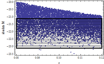
Angular size selection effects.
Whilst the volume-limited-sample method avoids the unwanted brightness-selection effects, additional caution has to be exercised when analyzing sizes, i.e. Petrosian radii of galaxies. Due to the target selection algorithm there is a necessary cut in angular size between stars and galaxies, and very few Petrosian radii lie below 2 arcsec (see fig. 5).

Without any precaution, this would bias the results, because at large distance, 2 arcsec correspond to a larger galaxy size than at close distance. To be sure, we remove therefore all galaxies from the data set, which would appear at a smaller angle than 2.2 arcsec at the maximum redshift. A similar procedure is applied by [11] to the smaller quantity .55 5 however is still more affected by seeing than the Petrosian radius [19], fig.4. The numerical value of the cut can be varied as a parameter in our code. It corresponds to a cutoff below a certain absolute size in kpc for the whole sample. Consequently, we also define an overall upper limit for galaxy size (about 20 kpc) to avoid data points with huge errors. Thus, analogous to the rectangular form of volume limited samples in a redshift-magnitude diagram, we additionally applied a corresponding rectangle in a redshift-size diagram for our analysis. Any pathology arising from improper selection should be avoided by these methods.
Density and luminosity anomalies.
It should be noted that, although all care has been exercised while selecting the data, the density of galaxies still does not correspond precisely to the naive assumption of a mean constant density at large scales. However, since it is generally established that the main galaxy sample is complete exceeding [20, 21], this cannot influence the results observed here.66 6 [22] describes the distribution of galaxies by a density parameter.
Independent of the problem investigated here, it was recently found that galaxy luminosity clearly increases with [18, 22, 23]. This is in principle consistent with models of of stellar evolution, although a quantitative understanding is still missing. Usually, the effect is described by an evolution parameter, determined by [22] to be per unit redshift for the band . Thus, in our code we allow for this luminosity evolution, and include 1.62 as a variable parameter.
2.4 K-correction
The discussion so far is based on the assumption that the magnitudes in the respective filters are comparable at different redshifts. Unfortunately, this is not true, since light of a distant galaxy which was originally say in the or even filter, due to the Hubble redshift is detected in the filter.77 7 E.g., a redshift would shift the center to the center . This distance-dependent effect needs careful treatment, called -correction, and various groups studied in detail how the filter magnitudes transform into the rest system [24, 19]. We use the values from the photo table in SDSS. An approximation of similar quality, but based on a simpler technique, is described in [25], where a fifth-order polynomial in and (difference of magnitudes in the and filter) nicely reproduces the more detailed analysis. Since it is easily accessible, the polynomial approximation is implemented in our code as well (see appendix).
2.5 The impact of seeing on the Petrosian radius
Another considerable problem for obtaining reliable Petrosian radii is the effect of seeing. It is obvious that bad atmospheric conditions tend to smear out galaxy profiles. This is dangerous in principle, because the relative effect should be more pronounced at smaller angles and larger distances. Limited seeing could therefore mimic a size increase with redshift, as already noted in [20] (fig. 4). Unfortunately, seeing affects all angular-size measures. This even has been shown for the galaxy-light-concentration factor [26] 88 8 and denote the radii (in arcsec) where the respective percentage of the Petrosian magnitude is found (the Petrosian magnitude is defined by the light within two Petrosian radii).. Whilst is less dependent, every angular-distance measure tends to increase with seeing . To determine the relation between galaxy radius and seeing , we fit all pairs (see fig. 6) by a linear function, which yields a best-fit slope of about for the and filters. Thus, the ‘true’ Petrosian angle can be estimated individually by extrapolating to perfect seeing .

To test the dependence of the above seeing correction on outliers, we bin the data into intervals of width 0.1 in seeing . The medians of these bins yield 17 data points for . Those were weighted by the number of galaxies and again fitted by a linear function. We obtained 0.462 for the slope in and 0.483 for the slope in , a marginal difference to the above values (see fig.6).
2.6 The impact of color on the Petrosian radius
Besides the dependence on seeing, one also must consider the influence of redshift. The more prominent effect on magnitude is accounted for by the K-correction, but there could be an impact of the redshift on the Petrosian radius if the galaxy has different radii in different color bands. The idea to correct for this effect is to use to determine a linear interpolation of the and the radius which is independent of . First however, one has to assure that and are on average of the same size. After having corrected for seeing, we analyzed the ratio over redshift (fig. 7)

and found a slight dependence:
| (3) |
Taking this into account, the interpolation could be calculated as follows: Since redshift would transform the center of the filter () to the center of the filter (), our redshift dependent radius was computed as
| (4) |
To ensure using only absolutely reliable data, we remove all galaxies from the data set where and differ by more than .
Cosmological parameters.
Though we expressed our results in terms of redshift, angular diameter distances for the galaxies were necessary to correct both for the absolute magnitude and for the computation of the real size from the angular (Petrosian) radius. The distances (1) depend on the Hubble constant and on the densities of matter and dark energy . All quantities can be varied in our program as parameters. Thus the galaxy size in kpc is simply
| (5) |
where is the Petrosian angle in arcsec (r-band) and the absolute magnitude is
| (6) |
where , are the extinction-corrected magnitudes in the u,g,r,i,z filters and is the K-correction of [25], while ‘individual’ K-corrections from SDSS are considered as well.
2.7 Further selection criteria and data reduction
Several conflicting effects have to be balanced when selecting appropriate parameters for our investigation: 1) a larger range makes it easier to detect possible trends. 2) the number of systematic effects and their possible errors increases for large , e.g. the K-correction. 3) as evident from fig. 4, a large range leads to a small range in magnitudes and many galaxies are cut off by the volume limited sample method.
can be used as a variable parameter and the largest numbers of galaxies in the data set occur for . The number of galaxies is also used as a guiding principle for choosing the location of the galaxy sample. The peak of our original magnitude-limited () population is located at . Thus we concentrate our analysis on the interval to where most of the data points lie. Another parameter to choose is the thickness in magnitude of the ‘stripes’ used to divide the volume limited samples as in fig. 4. Given that peculiar velocities are in the range of which corresponds to a uncertainty , this leads to an error of almost 0.1 mag at . Therefore, we choose as default value.
A First approach: Linear fit of size trends.
We exemplarily look at one stripe and selected by the volume-limited-sample method described above (fig. 4). Though having the same absolute magnitude, the sizes of the galaxies differ considerably. The large scatter is illustrated in fig.8 (left). A linear least-square fit to the data points99 9 We required a minimum number of 300 galaxies in each stripe. yields a slope (in kpc/redshift), and an -axis intercept, which can be interpreted as the average radius of a galaxy with the given luminosity at .

Improved fit of bin medians.
As visible in fig. 8 (left), the scatter in size for galaxies of the same magnitude is considerable and may give rise to line-fit errors. Since the median is not sensitive to possible outliers, instead of fitting the data directly, as in fig. 8 (left), we first calculate the median of the Petrosian radii within small intervals , as shown in fig.8 (right), and then fit a line to these medians. This procedure reduces a data set like fig.8 (left) to points and avoids the otherwise implicit weighting by the number of galaxies that varies with redshift. There is however another subtlety that justifies this procedure. Due to the overall size cut to avoid outliers, e.g. only galaxies with are considered for . While this is appropriate for an average luminosity, a significant number of bright galaxies are cut by while the distribution of faint galaxies is affected by the cut . In this case, the mean radius overestimates the real value for faint galaxies, while the mean radius of the bright galaxies is distorted towards smaller values. For both effects, taking the median instead of the mean is the appropriate remedy. It is further clear the direct fit without median would underestimate any size trend (see Table 1). Thus we consider the median fit to be the cleaner procedure than fitting directly all data points in fig. 8 (left). Such a linear median fit is computed for every magnitude ‘stripe’. The slope of these functions is then a measure of size increase with .
But how to compare a size increase for galaxies with different sizes? Therefore, we choose as meaningful quantity the relative increase per unit redshift, . It will be of central importance in our results. However, a meaningful value for the reference radius at redshift has yet to be found. Though an individual linear fit yields a slope and an intersection estimating , the latter value, being an extrapolation, can have a large error. As it can be observed in a typical result like fig. 9, a smaller intersection leads to a higher slope and vice versa; we seeked an that avoided such an anticorrelation.

Determining a characteristic size-magnitude relation for galaxies.
To determine such a characteristic relation between magnitude and average size, we ran the above algorithm for various redshift intervals, resulting in a ensemble of estimates, as shown in fig. 9 (middle). Then we fit all these estimates by the 3-parameter (a,b,c) nonlinear function(see later fig. 10):
| (7) |
The characteristic size-magnitude relation obtained in this way provides a reasonable yardstick for subsequent runs of the algorithm, where the central quantity now refers to this (see fig. 10 below). Technically, it is of advantage to use a more precise characteristic size-magnitude relation determined at , instead to the extrapolated radii at . In this case, we however had to apply a correction for the on average larger radii at .
Properties of the size distribution.
As an additional test, we were interested if the size distributions of galaxies at different redshift showed a suspicious behaviour. E.g., a narrower distribution with increasing median would indicate an artificial cut of a population of galaxies. A typical result is shown in fig. 9 (right).
3 Results
Characteristic galaxy sizes .
The relation between average size and magnitude is obtained by the 3-parametric fit described in the last section. For the parameters in (7) we find for , , and , , for . Altogether, we found the following dependence fig. 10. Given the uncertainties, a quite consistent function may be drived from (depending on , here ).

Main result: galaxy size change with .
The results of our redshift-size analysis are shown in figs. 11-12, each small picture for a different redshift regime. The negative values of indicate an average size decrease with redshift , equivalent to a growth in time.

The trend is less pronounced at higher redshift but occurs at all magnitudes. While in fig. 11 the average of over all magnitudes is given, one could think about weighting. Since the number of galaxies decreases dramatically with magnitude, weighting by the number would lead to faint galaxies dominating the result. As a compromise, often used in statistics, a square-root-weighted average is also considered, all these quantities are displayed in the summary Table 1. It is quite natural that the few bright galaxies show a relatively larger scatter (see fig. 9 right). While fig. 11 refers to the K-correction provided by SDSS, we repeated our analysis with a simple polynomial expression for the K-correction given by [25] depending on and filter magnitudes only. Thereby, the average of is slightly increased (see summary of results). The remarkable difference is that SDSS provides positive values for the correction without exception, while the polynomial expression by [25] yields a considerable number of negative values at small redshifts. Another type of K-correction depending on the and filter (instead of and ) results only in insignificant changes (not shown here), while without K-correction (a physically unmotivated case) the effect is masked. The effect of color due to different redshifts on the value of the Petrosian radius turned out to be negligible.
Taking into account luminosity evolution.
Given the findings of [22] on the redshift dependence of the luminosity function1010 10 The distribution of galaxies over the range of luminosities is usually fitted with a Schechter function., we were also interested whether our effect could be understood as a consequence of it. Instead of taking stripes of equal luminosity in fig. 4, we were considering a sample of galaxies with increasing luminosity in z (-1.62 mag per unit z in the r-band [22]). However, since magnitude and size are correlated, this led to a selection of brighter and therefore bigger galaxies at higher redshift. Thus the average size increases now with , correspinding to a shrinking in time, as shown in fig. 12.

It seems to be difficult to explain within the common picture of galaxy evolution.
Cosmological parameters.
As expected, the results depend on the Hubble constant, though quite moderately see Table 1. and fig. 13. Additionally, we varied from to while keeping fixed, with a still smaller effect than for varying . Plotting all possible parameter variations and their combinations would require excessive space. Most of the applied correction methods had an impact on the results. Cutting out the rectangular volume limited samples from fig. 4 led to smaller values of , and so did the consideration of the angular size limits.

Seeing.
The cutoff value in the Petrosian angle due to the star-glaxy separation turned out to be significant in principle, but the value of 2.2 arcsec carefully chosen. Changing it to 2.7 arcsec decreased significantly the number of galaxies in the analysis, but not did not influence the results very much.
Statistical errors.
In view of the clear significance of the effect we did not perform a detailed statistical analysis. Rather it is illustrative to demonstrate the impact of a large statistical scatter on our results. To introduce noise, it suffices to choose parameters obviously outside a reasonable ranage. E.g., the thickness of the magnitude stripes could be chosen much inferior to the typical error in magnitude due to peculiar velocities (see fig. 14)

Summary of results.
Based on the detailed results displayed in fig .11-12, we give summary in table 1. The influence of absolute magnitude M is now included in different ways of averaging .
| z range | 0.07-0.11 | 0.08-0.12 | 0.09-0.13 | 0.06-0.12 | 0.07-0.13 | 0.08-0.14 |
|---|---|---|---|---|---|---|
| Default (fig. 11) | ||||||
| average | -0.56 | -0.49 | -0.17 | -0.38 | -0.40 | -0.24 |
| sqrt-weighted av. | -0.50 | -0.46 | -0.23 | -0.46 | -0.38 | -0.29 |
| weighted av. | -0.48 | -0.46 | -0.28 | -0.52 | -0.36 | -0.33 |
| K-corr. polynomial: | ||||||
| average | -0.61 | -0.58 | -0.24 | -0.45 | -0.5 | -0.38 |
| sqrt-weighted av. | -0.54 | -0.53 | -0.27 | -0.52 | -0.47 | -0.38 |
| weighted av. | -0.50 | -0.53 | -0.31 | -0.57 | -0.45 | -0.40 |
| No K-correction: | ||||||
| average | -0.07 | 0.26 | 0.46 | 0.20 | 0.14 | 0.2 |
| sqrt-weighted av. | -0.04 | 0.21 | 0.34 | 0.07 | 0.09 | 0.28 |
| weighted av. | -0.03 | 0.16 | 0.26 | -0.03 | 0.05 | 0.28 |
| : | ||||||
| average | -0.30 | -0.16 | -0.02 | -0.34 | -0.16 | -0.06 |
| sqrt-weighted av. | -0.36 | -0.3 | -0.08 | -0.40 | -0.22 | -0.09 |
| weighted av. | -0.39 | -0.38 | -0.12 | -0.47 | -0.22 | -0.12 |
| Fit without median: | ||||||
| average | -0.30 | -0.18 | -0.02 | -0.24 | -0.13 | -0.05 |
| sqrt-weighted av. | -0.36 | -0.23 | -0.02 | -0.27 | -0.18 | -0.06 |
| weighted av. | -0.38 | -0.26 | -0.02 | -0.31 | -0.2 | -0.07 |
| Cut at 2.7 arcsec: | ||||||
| average | -0.54 | -0.48 | -0.22 | -0.38 | -0.44 | -0.22 |
| sqrt-weighted av. | -0.47 | -0.44 | -0.29 | -0.45 | -0.43 | -0.27 |
| weighted av. | -0.42 | -0.43 | -0.34 | -0.49 | -0.43 | -0.31 |
| Evolution (fig. 12) | ||||||
| average | -0.04 | 0.24 | 0.51 | 0.21 | 0.26 | 0.45 |
| sqrt-weighted av. | 0.05 | 0.20 | 0.46 | 0.12 | 0.26 | 0.45 |
| weighted av. | 0.09 | 0.15 | 0.41 | 0.04 | 0.26 | 0.43 |
| z range | 0.07-0.11 | 0.08-0.12 | 0.09-0.13 | 0.06-0.12 | 0.07-0.13 | 0.08-0.14 |
Table 1.
Relative increase of galaxy size per unit redshift, . Average taken over
different magnitudes, weigthed and sqrt-weighted with the number of galaxies, corresponding
to fig. 11. Default refers to: K-correction from SDSS photo z table, fit of medians,
no luminosity evolution, angular cut at arcsec, size limit .
4 Discussion
We developed a method to analyze for galaxy-size evolution at low redshifts. We find a slight decrease of average galaxy size with redshift, corresponding to a growth in time. This result does not depend on galaxy luminosity, indicating that the various corrections applied were reasonable. The fact that this decrease is less pronounced at higher redshifts is more difficult to interpret and may be due bias from the K-correction. However, none of the different K-correction methods tested made the anomaly disappear. The same holds for different values of . While a smaller , corresponding to an older universe, yields a smaller change in size, the effect does not disappear. The fit without taking the median and the cut at slightly masks a change for the reasons given above. It is however very interesting to see that the trend in size change is reversed when taking into account the luminosity evolution [22]. Because there is obvious physical explaining the luminosity evolution, we cannot decide which of the two puzzling effects, size or luminosity change, is real. While luminosity increase could originate from stellar processes, a change in size is more difficult to understand. In any case, future analyses should consider both effects.
With respect to other results regarding size evolution, our finding of a slight increase in time would correspond to the observation of too small galaxies at very high redshift (e.g. [4]), though a quantitative agreement cannot be deduced yet. Looking at fig. 1, it is clear that those results challenge the angular-size-redshift-relation of the model in particular at high redshift. It is also clear that such an effect is less pronounced at low redshifts where our analysis took place.
A pragmatic approach would be to introduce an independent parameter describing physical processes leading to the observed growth. Methodologically, this is dangerous because for galaxies we only have a limited number of observable quantities: redshift, number density, luminosity and size. On the other hand, we observe an anomalous density, a luminosity evolution and unexpected changes in size. It is not evident how a comprehensive understanding of these effects can be obtained within standard cosmology.
5 Outlook
We have here developed a quantitative method to identify galaxy size evolution at small redshift. Our results present yet another riddle for the study of galaxies. We hope that our published code will facilitate further investigations of this effect.
Acknowledgement.
We are grateful to Francesco Sylos Labini and Martin Lopez-Corredoira for helpful hints and thank Simon Staude for assistance. A.U. thanks for the comments of David Hogg, Tom Shanks, Rudi Schild, Vladimir Sokolov and Rick Watkins during the conference ‘New directions in modern cosmology’ and and the Lorentz Center in Leiden for the hospitality.
References
- [1] C. Nipoti et.al. Can Dry Merging Explain the Size Evolution of Early-Type Galaxies? Astrophysical Journal Letters, 706:L86–L90, 2009, arXiv: 0910.2731.
- [2] S. K. Banerjee and J. V. Narlikar. The quasi-steady-state cosmology: a study of angular size against redshift. Mon. Not. R. Astr. Soc., 307:73–78, 1999.
- [3] F. Shankar et.al. Sizes and ages of SDSS ellipticals: comparison with hierarchical galaxy formation models. MNRAS, 403:117–128, 2010, arXiv: 0912.0012.
- [4] M. López-Corredoira. Angular Size Test on the Expansion of the Universe. International Journal of Modern Physics D, 19:245–291, 2010, arXiv:1002.0525.
- [5] D. Raine and E. G. Thomas. An Introduction to the Science of Cosmology. Taylor and Francis, 2002.
- [6] E. Harrison. Cosmology: The Science of the Universe. Cambridge University Press, 2002.
- [7] D. E. Friedmann. Dark matter redistribution explains how galaxies grow in size and develop characteristic rotation curves. arXiv: 0912.1668.
- [8] S. Wuyts et.al. On Sizes, Kinematics, M/L Gradients, and Light Profiles of Massive Compact Galaxies at z˜2. 2010, arXiv: 1008.4127.
- [9] L. I. Gurvits, K. I. Kellermann, and S. Frey. The “angular size - redshift” relation for compact radio structures in quasars and radio galaxies. Astronomy and Astrophysics, 342:378–388, 1999, astro-ph/9812018.
- [10] P. B. et.al. Nair. The environmental dependence of the luminosity-size relation for galaxies. 2010, arXiv: 1004.1107.
- [11] S. Shen et.al.n. The size distribution of galaxies in the sloan digital sky survey. 2003, astro-ph/0301527.
- [12] M. Takamiya. Galaxy Structural Parameters: Star Formation Rate and Evolution with Redshift. Astrophysical Journal Supplement, 122:109–150, 1999.
- [13] SDSS team. Understanding the image processing flags - summary table. http://www.sdss.org/dr7/products/catalogs/flags.html, 2009.
- [14] C. H. Lineweaver et.al. The Dipole Observed in the COBE DMR 4 Year Data. Astrophysical Journal, 470:38–+, 1996, astro-ph/9601151.
- [15] A. Sandage and L. M. Lubin. The Tolman Surface Brightness Test for the Reality of the Expansion. I. Calibration of the Necessary Local Parameters. Astronomical Journal, 121:2271–2288, 2001, astro-ph/0102213.
- [16] V. Petrosian. Surface brightness and evolution of galaxies. Astrophysical Journal Letters, 209:L1–L5, 1976.
- [17] SDSS site. Photometry description. http://www.sdss.org/dr7/algorithms/photometry.html, 2009.
- [18] M. R. Blanton et.al. The Luminosity Function of Galaxies in SDSS Commissioning Data. Astronomical Journal, 121:2358–2380, 2001.
- [19] Blanton et.al. Estimating Fixed-Frame Galaxy Magnitudes in the Sloan Digital Sky Survey. Astronomical Journal, 125:2348–2360, 2003, astro-ph/0205243.
- [20] M. A. Strauss et. al. Spectroscopic Target Selection in the Sloan Digital Sky Survey: The Main Galaxy Sample. Astronomical Journal, 124:1810–1824, 2002, astro-ph/0206225.
- [21] A. H. Maller et.al. The Intrinsic Properties of SDSS Galaxies. Astrophysical Journal, 691:394–406, 2009, arXiv:0801.3286.
- [22] Blanton et.al. The Galaxy Luminosity Function and Luminosity Density at Redshift z = 0.1. Astrophysical Journal, 592:819–838, 2003, astro-ph/0210215.
- [23] J. Loveday. Evolution of the galaxy luminosity function at z ¡ 0.3. MNRAS, 347:601–606, 2004, astro-ph/0309429.
- [24] D. W. Hogg et.al. The K correction. 2002, astro-ph/0210394.
- [25] Chilingarian et.al. Analytical approximations of k-corrections in optical and near-infrared bands. 2010, arXiv: 1002.2360.
- [26] M. R. Blanton et. al. The Broadband Optical Properties of Galaxies with Redshifts . Astrophysical Journal, 594:186–207, 2003, astro-ph/0209479.
Source codes
SQL query.
With the commands given below, all the data used in our analysis can be downloaded from the SDSS site . By taking away the top 20 constraint in the first row, the search will however produce a timeout due to the exeeding of the SDSS row limit of 100000 lines. Therefore, the z range has to be split up in different queries. A good idea is to choose small ranges, typically 0.01 or even smaller. Check if there is no timeout error, and save all the files in one directory without renaming them. A Mathematica routine how to join the files again is given below.
-- this indicates a comment.
-- top 20 is just for a check. It has to be taken out later
select top 20 s.ra, s.dec, s.z as redshift, s.zconf,
(p.petroMag_u - p.extinction_u) as mag_u,
(p.petroMag_g - p.extinction_g) as mag_g,
(p.petroMag_r - p.extinction_r) as mag_r,
p.petroRad_g, p.petroRad_r,
p.petroRadErr_g, p.petroRadErr_r,
p.petroR50_g, p.petroR50_r,
p.petroR90_g, p.petroR90_r,
r.seeing_g, r.seeing_r,
h.kcorr_g, h.kcorr_r,
h.absMag_g, h.absMag_r
from galaxy p, specObj s, RunQA r, Photoz h
where p.objID = s.bestObjID and
p.fieldID = r.fieldID and
p.objID = h.objID and
-- s.specClass=2 and
s.z BETWEEN 0.0001 AND 0.02   --to be adjusted in steps:  0.03, 0.035, 0.04, 0.045...0.06,0.064,0.068,
-- 0.072, 0.076, .....0.10,0.105, ...0.
AND p.objID <> 0
AND (p.petroMag_r - p.extinction_r) < 17.77 -- faint magnitude limit for MGS
AND ((flags_r & 0x10000000) != 0)
-- detected in BINNED1
AND ((flags_r & 0x8100000c00a0) = 0)
-- not NOPROFILE, PEAKCENTER, NOTCHECKED, PSF_FLUX_INTERP, SATURATED,
-- or BAD_COUNTS_ERROR.
-- if you want to accept objects with interpolation problems for PSF mags,
-- change this to: AND ((flags_r & 0x800a0) = 0)
AND (((flags_r & 0x400000000000) = 0) or (psfmagerr_r <= 0.2))
-- not DEBLEND_NOPEAK or small PSF error
-- (substitute psfmagerr in other band as appropriate)
AND (((flags_r & 0x100000000000) = 0) or (flags_r & 0x1000) = 0)
-- not INTERP_CENTER or not COSMIC_RAY - omit this AND clause if you want to
-- accept objects with interpolation problems for PSF mags.
-- AND ((flags_r & 0x0000000000800000) = 0) -- petrofaint
-- AND ((flags_r & 0x0000000000000100) = 0) -- nopetro
AND ((flags_r & 0x0000000000000400) = 0) -- nopetro_big
-- AND ((flags_r & 0x0000000000000200) = 0) -- manypetro
AND ((flags_r & 0x0000000000002000) = 0) -- manyr50
AND ((flags_r & 0x0000000000004000) = 0) -- manyR90
AND ((flags_r & 0x0000000100000000) = 0) -- DEBLENDED_AS_MOVING
AND ((flags_r & 0x0000000000400000) = 0) -- badsky
order by s.z
Mathematica code - preliminaries.
The following commands which work irrespective of the names given to the downloaded files produce a datafile of the type we used. The CMB correction is also calculated here. You need to name your working directory accordingly. Writing several files of about 100 MB and the CMB calculation may need considerable time up to 30 mins. This has to be done only once, however.
Needs["VectorAnalysis‘"];(* glueing files with different ranges to one file:
store your SDSS datafiles like result (13).csv in a separate subdircetory named sdssgals*)
mydir ="c:\\Users\\sascha\\Desktop\\sdss\\";(* replace this with your math dir*)
SetDirectory[mydir <> "sdssgals"];
li = FileNames[];
compl = {{"ra", "dec", "redshift", "zconf", "mag_u", "mag_g", "mag_r",
    "petroRad_g", "petroRad_r", "petroRadErr_g", "petroRadErr_r",
   "petroR50_g",  "petroR50_r", "petroR90_g",  "petroR90_r",
   "seeing_g", "seeing_r", "kcorr_g", "kcorr_r", "absMag_g",
   "absMag_r"}}; For[kk = 1, kk <= Length[li], kk++,
 wer = Drop[Import[li[[kk]], "CSV"], 1];
 AppendTo[compl, wer]]; out = Flatten[compl, 1];
SetDirectory["c:\\Users\\sascha\\Desktop\\sdss"];
(*Export["allgal.csv",out,"CSV"];*)out >> "allgal.txt";
allGalaxies = Drop[<< "allgal.txt", {1, 21}];
(* CMB correction: 10 min, for that stored in separate file*)
CMBShift[x_] :=Block[{dis, halb},
dis = CoordinatesToCartesian[{1, Pi/2 - Pi (x[[2]])/360, Pi (x[[1]])/360}, Spherical] -
CoordinatesToCartesian[{1, Pi/2 - Pi 7.22/360, Pi 167.99/360}, Spherical];
halb = ArcTan[Sqrt[Plus @@ (dis^2)]/2];
zadd = Round[0.00123*Cos[2 halb], 0.000001]];
xx = OpenWrite["allGalCMB2.txt"];
For[ii = 1, ii <= Length[allGalaxies], ii++, linie = allGalaxies[[ii]];
 add = CMBShift[linie];
 linie3 = ReplacePart[linie, {3 -> linie[[3]] + add}];
 WriteString[xx, linie3[[3]], " ", linie3[[4]], " ", linie3[[5]], " ",
   linie3[[6]], " ", linie3[[7]], " ", linie3[[8]], " ", linie3[[9]],
  " ", linie3[[10]], " ", linie3[[11]], " ", linie3[[16]], " ",
  linie3[[17]], " ", linie3[[18]], " ", linie3[[19]], " ",
  linie3[[20]], " ", linie3[[21]]];
 Write[xx]]; Close[xx];
Mathematica code - main analysis.
The first paragraph still contains preliminaries that need not to be run every time. At the very first run, the comment (*.. *) has to be dropped in line 12-14 in order to produce the file galBuff.txt, which is smaller and can be used in the following.
mydir = "c:\\Users\\sascha\\Desktop\\sdss";(* put your working directory here*)
SetDirectory[mydir]; Needs["Combinatorica‘"]; Needs["ANOVA‘"];
Needs["StatisticalPlots‘"];
cc = 299792.458; minmag = 17.5; maxmag = 14.5;(* speed of light and mag range*)
xq = Table[{}, {20}];(*contains graphics*)
LimitedSample[lst_, lim_] :=
 Select[lst, (#[[lim[[1]]]] >= lim[[2]] && #[[lim[[1]]]] <=lim[[3]]) &];
LimitedSample2p[lst_, lim1_, lim2_] :=
Select[lst, (#[[lim1[[1]]]] >= lim1[[2]] && #[[lim1[[1]]]] <=
      lim1[[3]] && #[[lim2[[1]]]] > lim2[[2]] && #[[lim2[[1]]]] <= lim2[[3]]) &];
(*allGalaxies=Import["allgalCMB2.txt","Table"];tu=TimeUsed[];*)
(*vorgal=LimitedSample2p[allGalaxies,{5,maxmag, minmag+0.27},{2,0.9, 1.0}];
gal=LimitedSample2p[vorgal,{8,0,5},{9,0,5}]; gal>>"galBuff,txt";*)
(** starting with fainter than 17.5, otherwise kcorr diluites distribution*)
gal = << "galBuff.txt";
tgoR = Transpose[gal];
SeeAndPetg = Transpose[{tgoR[[10]], tgoR[[6]]}];
seeFit =Fit[SeeAndPetg, {1, x}, x]; psightg = seeFit[[2, 1]];
SeeAndPetr = Transpose[{tgoR[[11]], tgoR[[7]]}];
seeFit = Fit[SeeAndPetr, {1, x}, x]; psightr = seeFit[[2, 1]];
tgoR = Drop[Insert[tgoR, tgoR[[6]] - tgoR[[10]] psightg, 6], {7}];
tgoR = Drop[Drop[Drop[Insert[tgoR, tgoR[[7]] - tgoR[[11]] psightr, 7], {8}], -2], {10, 11}];
gal2 = Transpose[tgoR]; (* not everything is needed*)
grRatio = 1.0149; grSlope = 0.10095;
(*grpetrotest=Transpose[{tgoR[[1]],tgoR[[6]]/tgoR[[7]]}];
Fit[grpetrotest,{1,x},x]*)
(*** K-correct Polynomials Chilingarian et al. 2010*)
rWithgr = {{0, 0, 0, 0}, {-1.61166, 3.87173, -3.87312,
    2.66605}, {8.48781,
    13.2126, -6.4946, -7.31552}, {-87.2971, -35.0474, 41.5335,
    0}, {271.64, -26.9081, 0, 0}, {-232.289, 0, 0, 0}};
rWithur = {{0, 0, 0, 0}, {-1.98173, 1.04346,
    0.0221613, -0.0391318}, {9.34198, 1.639, -0.392805,
    0.192349}, {-39.8237, -10.3007, -1.9142, 0}, {123.94, 25.7117, 0,
    0}, {-150.964, 0, 0, 0}};
koeff = Table[c^i z^j, {j, 0, 5}, {i, 0, 3}];
KcorrRgr[c_, z_] = Plus @@ Flatten[rWithgr koeff];
KcorrRur[c_, z_] = Plus @@ Flatten[rWithur koeff];
The following input defines the main routine Petroplot. All parameters can be varied here.
(*cosmological parameters, mag range, absolute mags considered, z range, minimum number of galaxies*)
PetroPlot[{H0_, Om_, OL_}, magstep_, {minz_, maxz_, dz_}, {minpetro_, maxsize_},
   minnumber_, {petroErr_, petroRatio_}, kflag_, distflag_, Rflag_, fitflag_, Epar_] :=
  Block[{zselect, zselectK, pselect, goodRad, seeingcorr},
   tu1 = TimeUsed[]; (* v1 corrected*)
   EmmissionDistInt2[z_] :=1/(1 + z) cc/H0 NIntegrate[1/(OL+(1+x)^3*Om),{x, 0, z}];
   If[distflag == 1,EmmissionDist =Interpolation[Table[{z, EmmissionDistInt2[z]}, {z, 0, 5, .02}]],
    Clear[EmmissionDist]; EmmissionDist[z_] = z*cc/2/H0 ];
   DistCorrect[z_] := -5 Log[10, (1+z)^2 EmmissionDist[z]] - 25; (* v1 corrected*)
   AbsPetR[tg_] :=EmmissionDist[tg[[1]]]*1000 *((tg[[6]] + (tg[[7]]*grRatio - tg[[6]])*
          tg[[1]] (grSlope + 1/0.30608)) /3600) Pi/180 ;
(* Galaxy sizes in kpc: now considering the shift from the g-band to the r-band*)
   (* redshift .30608 would shift the center of g to the center of r
   grratio is accounts for the ration of average g/r radii*)
   zselect = LimitedSample[gal2, {1, minz, maxz}];
   (* selecting z range and sufficient seeing conditions *)
(*now substituting with reduced pretorad due to seeing *)
   Print["correcting for seeing with coefficients g,r: ", {psightg, psightr}];
   goodRad = Select[zselect, (1/petroRatio < #[[7]]/#[[6]] < petroRatio) &];
   pselect = Select[goodRad, ((#[[8]]/(#[[6]]) <
          petroErr) && (#[[9]]/(#[[7]]) <
          petroErr) && ((#[[6]] + (#[[7]]*grRatio - #[[6]])*#[[1]] (grSlope + 1/0.30608)) >
          minpetro*EmmissionDist[maxz]/
       EmmissionDist[#[[1]]]) && ((#[[6]] + (#[[7]]*grRatio - #[[6]])*#[[1]] (grSlope + 1/0.30608))*
       1000/3600*Pi/180*EmmissionDist[#[[1]]] < maxsize)) &];
(*dropping huge errors in petrorad*)
   (* taking out all galaxies that would appear at < minpetro at
   the maximum redshift, thus avoiding a size bias *)
   (*taking a linear combination of the radii in the r and g band*)
   Print[
    "Total sample/z+faint mag/ petro constraints: ", {Length[gal],
     Length[zselect], Length[pselect]}];
   Kcorr[c_, z_] :=
    Switch[kflag, 0, 0, 1, KcorrRgr[c, z], 2, KcorrRur[c, z]];
   usedData = {#[[1]],
       EmmissionDist[#[[1]]], #[[5]] + DistCorrect[#[[1]]] -
        If[kflag == -1, #[[11]],
         Kcorr[#[[5 - kflag]] - #[[5]], #[[1]]]] + (#[[1]] - 0.1)*
         Epar, AbsPetR[#]} & /@ pselect;
   (* only redshift, distance,
   luminosity and size in the following *)
   (* now accounting for evolution , Blanton et. al.2003:*)
   (* determination of reasonable magnitudes in the given z range *)
   minabs = minmag + DistCorrect[maxz];
   maxabs = maxmag + DistCorrect[minz];
   Print["Original Range: ", {minabs, maxabs}];
   slices =Table[Select[
      usedData, ((ii >= #[[3]]) &&  #[[3]] > ii - magstep) &], {ii,
      minabs, maxabs, -magstep}];
   lastslice = Mod[minabs - maxabs, magstep];
   (* take out the sets with a small galaxy number*)
   While[Length[slices[[1]]] < minnumber, slices = Delete[slices, 1];
    minabs -= magstep];
   count = 0;(*
   taking into account that the last slice could be smaller than magstep*)
   While[Length[slices[[-1]]] < minnumber,
    slices = Delete[slices, -1];
    maxabs += If[count == 0, lastslice, magstep]; count += 1;];
   mla = Map[Length, slices];
   mags = Take[Table[j, {j, minabs, maxabs, -magstep}] - magstep/2, {1,
      Length[mla]}];
   pairstab = Table[{Mean[#[[3]] & /@ slices[[i]]],
      Map[{#[[1]], #[[4]]} &, slices[[i]]]}, {i, 1, Length[slices]}];
   chest = Table[{pairstab[[i, 1]],
      Select[pairstab[[i,
        2]], (minz + k*dz < #[[1]] < minz + (k + 1)*dz) &]}, {k,
      0, (maxz - minz)/dz - 1}, {i, 1, Length[pairstab]}];
   mags = Table[chest[[i, k, 1]], {k, 1, Length[chest[[1]]]}, {i, 1,
      Length[chest]}];
   zMedi =
    Table[Median[Transpose[chest[[i, k, 2]]][[1]]], {k, 1,
      Length[chest[[1]]]}, {i, 1, Length[chest]}];
   newVari =Table[Sqrt[Variance[Transpose[chest[[i, k, 2]]][[2]]]], {k, 1,
      Length[chest[[1]]]}, {i, 1,
      Length[chest]}];
   newMedi =
    Table[Median[Transpose[chest[[i, k, 2]]][[2]]], {k, 1,
      Length[chest[[1]]]}, {i, 1, Length[chest]}];
   Medians =
    Table[{mags[[k, i]], {zMedi[[k, i]], newMedi[[k, i]]}}, {k, 1,
      Length[chest[[1]]]}, {i, 1, Length[chest]}];
   Variances =
    Table[{mags[[k, i]], {zMedi[[k, i]], newVari[[k, i]]}}, {k, 1,
      Length[chest[[1]]]}, {i, 1, Length[chest]}];
   newTabOfFits =
    Select[Table[{Medians[[j, 1, 1]],
       Fit[If[fitflag == 0, pairstab[[j, 2]],
         Transpose[Medians[[j]]][[2]]], {1, x}, x]}, {j,
       Length[Medians]}], NumberQ[#[[2, 1]]] == True &];
   newTabOfFitsV =
    Select[Table[{Variances[[j, 1, 1]],
       Fit[Transpose[Variances[[j]]][[2]], {1, x}, x]}, {j,
       Length[Variances]}], NumberQ[#[[2, 1]]] == True &];
   RelincR =
    If[Rflag == 0,
     Map[{#[[1]], #[[2, 2, 1]]/#[[2, 1]] } &, newTabOfFits],
     Map[{#[[1]], #[[2, 2, 1]]/SizeMag10[#[[1]]] } &, newTabOfFits]];
   RelincV =
    If[Rflag == 0, Map[{#[[1]], #[[2, 2, 1]] } &, newTabOfFitsV],
     Map[{#[[1]], #[[2, 2, 1]]} &, newTabOfFitsV]];
   R0 = Map[{#[[1]], #[[2, 1]] } &, newTabOfFits];
   R10 = Map[{#[[1]], #[[2]] /. x -> 0.1 } &, newTabOfFits];
   rp = ListPlot[R0, Frame -> True, Axes -> False,
     FrameLabel -> {"M", "kpc"}, PlotRange -> {0, 20}, Frame -> True,
     PlotLabel -> "average size at z=0"];
   weiAv = Round[Plus @@ ((#[[2]] & /@ RelincR)*mla)/Plus @@ mla, 0.01];
   sqrAv = Round[Plus @@ ((#[[2]] & /@ RelincR)*Sqrt[mla])/Plus @@ Sqrt[mla],0.01];
   avraw = Mean[Transpose[RelincR][[2]]];
   avV = Median[Transpose[RelincV][[2]]];
   av = Round[If[Rflag == 0, avraw, avraw/(1 - 0.1 avraw)], 0.01];
   sqav = Round[If[Rflag == 0, sqrAv, sqrAv/(1 - 0.1 sqrAv)], 0.01];
   weav = Round[If[Rflag == 0, weiAv, weiAv/(1 - 0.1 weiAv)], 0.01];
   Print[Plus @@ mla, " Galaxies of ", Length[pselect], " considered"];
   Print["in the absM range: ", {minabs, maxabs}];
   Print["Distribution: ", mla];
   Print["Weighted Average dR/R/dz: " , weav];
   Print["Sqrt-Average dR/R/dz: " , sqav];
   Print["average dR/R/dz: " , av]; tu2 = TimeUsed[];
   Print["time used: " , tu2 - tu1];
   pp = ListPlot[RelincR, Frame -> True, Axes -> False,
     FrameLabel -> {"M", "dR/R/dz"}, PlotRange -> {-3, 3},
     PlotLabel ->
      ToString[Plus @@ mla] <> " gal, av: " <> ToString[av]];
   pV = ListPlot[RelincV, Frame -> True, Axes -> False,
     FrameLabel -> {"M", "d sig /dz"}, PlotRange -> All,
     PlotLabel -> "av SD incr.: " <> ToString[Round[avV, 0.01]]]];
Now, the code can be run and visualized with
PetroPlot[{72, 0.3, 0.7}, 0.2, {0.08, 0.12, 0.0025}, {2.2, 20}, 300, {0.2, 1.2}, -1, 1, 0, 1, 0];
Show[GraphicsArray[{pp, rp, pV}]]
However, for our final resultes we used , which needs a function to be calculated by the following procedure which stores the characteristic radii in a file. Afterwards, Pertrorad can be repeated with Rflag=1 (third parameter from behind)
(** first step of determination of standardradii in the rest system Rflag=0*)
StandardRadii = StandardRadii10 = {}; For[i = 0, i <= 4, i++,
 PetroPlot[{72, 0.3, 0.7},
  0.2, {0.04 + 0.02 i, 0.08 + 0.02 i, 0.0025}, {2.2, 20},
  300, {0.2, 1.2}, -1, 1, 0, 1, 0]; Print[i];
 (*weighting where more galaxies are *)
 For[kk = 4, kk > i, kk--, AppendTo[StandardRadii, {R0, mla}]];
 For[kk = 4, kk >= (i - 2)^2, kk--,
  AppendTo[StandardRadii10, {R10, mla}]]];
{StandardRadii, StandardRadii10} >>"SRadiiK.txt";
(*or get it from data*)
{StandardRadii, StandardRadii10} = <<"SRadiiK.txt";
R0List = Flatten[#[[1]] & /@ StandardRadii, 1];
R10List = Flatten[#[[1]] & /@ StandardRadii10, 1];
(* function necessary to run with Rflag=1*)
SizeMag[m_] =
 Exp[Fit[{#[[1]], Log[#[[2]]]} & /@ R0List, {1, m, m^2}, m]];
SizeMag10[m_] =
 Exp[Fit[{#[[1]], Log[#[[2]]]} & /@ R10List, {1, m, m^2}, m]];
rlp = ListPlot[R0List, PlotRange -> {0, 20}, Frame -> True,
  PlotLabel -> "Standard radii z=0"]; smlp =
 Plot[SizeMag[m], {m, -22.7, -20.0}, PlotRange -> {0, 20},
  Frame -> True];
rlp10 = ListPlot[R10List, PlotRange -> {0, 20}, Frame -> True,
  PlotLabel -> "Standard radii z=0.1"]; smlp10 =
 Plot[SizeMag10[m], {m, -22.7, -20.0}, PlotRange -> {0, 20},
  Frame -> True];
g0 = Show[rlp, smlp]; g10 = Show[rlp10, smlp10];
xq[[5]] = Show[GraphicsArray[{g0, g10}], FrameLabel -> {"M", "kpc"}]
Now, run again
PetroPlot[{72, 0.3, 0.7}, 0.2, {0.08, 0.12, 0.0025}, {2.2, 20}, 300, {0.2, 1.2}, -1, 1, 1, 1, 0];