Fast Bivariate P-splines: the Sandwich Smoother

Luo Xiao ^†^†thanks: Graduate student, Department of Statistical Science, Malott Hall, Cornell University, New York 14853 (email: lx42@cornell.edu). Yingxing Li ^†^†thanks: Graduate student, Department of Statistical Science, Malott Hall, Cornell University, New York 14853 (email: yl377@cornell.edu). and David Ruppert ^†^†thanks: Andrew Schultz, Jr., Professor of Engineering, School of Operational Research and Information Engineering, Comstock Hall, Cornell University, New York 14853 (email: dr24@cornell.edu).

July 13, 2012

Abstract

We propose a fast penalized spline method for bivariate smoothing. Univariate P-spline smoothers (Eilers and Marx, 1996) are applied simultaneously along both coordinates. The new smoother has a sandwich form which suggested the name “sandwich smoother” to a referee. The sandwich smoother has a tensor product structure that simplifies an asymptotic analysis and it can be fast computed. We derive a local central limit theorem for the sandwich smoother, with simple expressions for the asymptotic bias and variance, by showing that the sandwich smoother is asymptotically equivalent to a bivariate kernel regression estimator with a product kernel. As far as we are aware, this is the first central limit theorem for a bivariate spline estimator of any type. Our simulation study shows that the sandwich smoother is orders of magnitude faster to compute than other bivariate spline smoothers, even when the latter are computed using a fast GLAM (Generalized Linear Array Model) algorithm, and comparable to them in terms of mean squared integrated errors. We extend the sandwich smoother to array data of higher dimensions, where a GLAM algorithm improves the computational speed of the sandwich smoother. One important application of the sandwich smoother is to estimate covariance functions in functional data analysis. In this application, our numerical results show that the sandwich smoother is orders of magnitude faster than local linear regression. The speed of the sandwich formula is important because functional data sets are becoming quite large.

KEYWORDS: Asymptotics; Bivariate smoothing; Covariance function; GLAM; Nonparametric regression; Penalized splines; Sandwich smoother; Thin plate splines.

1 Introduction

This paper introduces a fast penalized spline method for bivariate smoothing. It also gives the first local central limit theorem for a bivariate spline smoother. Suppose there is a regression function $\mu(x,z)$ with $(x,z)\in[0,1]^{2}$ . Initially we assume that $y_{i,j}=\mu(x_{i},z_{j})+\epsilon_{i,j},1\leq i\leq n_{1},1\leq j\leq n_{2}$ , where the $\epsilon_{i,j}$ ’s are independent with $\textrm{E}\epsilon_{i,j}=0$ and $\textrm{E}\epsilon_{i,j}^{2}=\sigma^{2}(x_{i},z_{j})$ , and the design points $\{(x_{i},z_{j})\}_{1\leq i\leq n_{1},1\leq j\leq n_{2}}$ are deterministic; thus, the total number of data points is $n=n_{1}n_{2}$ and the data are on a rectangular grid. In Section 4 we relax the design assumption to fixed design points not in a regular grid and random design points. With the data on a rectangular grid, they can be organized into an $n_{1}\times n_{2}$ matrix $\mathbf{Y}$ . We propose to smooth across the rows and down the columns of $\mathbf{Y}$ so that the matrix of fitted values $\hat{\mathbf{Y}}$ satisfies

\hat{\mathbf{Y}}=\mathbf{S}_{1}\mathbf{Y}\mathbf{S}_{2},

(1)

where $\mathbf{S}_{1}$ ( $\mathbf{S}_{2}$ ) is the smoother matrix for $x$ ( $z$ ). So fixing one covariate, we smooth along the other covariate and vice versa, although the two smooths are simultaneous as implied by (1). Estimator (1) is similar in form to the sandwich formula for a covariance matrix, which suggested the name “sandwich smoother” to a referee. We have adopted this term.

The tensor product structure of the sandwich smoother allows fast computations, specifically of the generalized cross validation (GCV) criterion for selecting smoothing parameters; see Section 2.2. Dierckx (1982) proposed a smoother with the same structure as (1), but our asymptotic analysis and the fast implementation for the sandwich smoother are new. For smoothing two-dimensional histograms, Eilers and Goeman (2004) studied a simplified version of the sandwich smoother with special smoother matrices that lead to non-negative smooth for non-negative data. The fast method for the sandwich smoother can be applied to their method.

For bivariate spline smoothing, there are two well known estimators: bivariate P-splines (Eilers and Marx, 2003; Marx and Eilers, 2005) and thin plate splines, e.g., the thin plate regression splines (Wood, 2003). For convenience, the Eilers-Marx and Wood estimators will be denoted by E-M and TPRS, respectively. We use E-M without specification of how the estimator is calculated.

Penalized splines have become popular over the years, as they use fewer knots and in higher dimensions require much less computation than smoothing splines or thin plate splines. See Ruppert et al. (2003) or Wood (2006) for both methodological development and applications. However, the theoretical study of penalized splines has been challenging. An asymptotic study of univariate penalized splines was achieved only recently (Opsomer and Hall, 2005; Li and Ruppert, 2008; Claeskens et al., 2009; Kauermann et al., 2009; Wang et al., 2011). The asymptotic convergence rate of smoothing splines, on the other hand, has been well established; see Gu (2002) for a comprehensive list of references.

The theoretical study of penalized splines in higher dimension is more challenging. To the best of our knowledge, the literature does not contain central limit theorems or explicit expressions for the asymptotic mean and covariance matrix of $\hat{\mu}(x,z)$ for bivariate spline estimators of any kind. The sandwich smoother has a tensor product structure that simplifies asymptotic analysis, and we show that the sandwich smoother is asymptotically equivalent to a kernel estimator with a product kernel. Using this result, we obtain a central limit theorem for the sandwich smoother and simple expressions for the asymptotic bias and variance.

For smoothing of array data, the generalized linear array model (GLAM) by Currie et al. (2006) gives a low storage, high speed algorithm by making use of the array structures of the model matrix and the data. The E-M estimator can be implemented with a GLAM algorithm (denoted by E-M/GLAM). The sandwich smoother can also be extended to array data of arbitrary dimensions where a GLAM algorithm can improve the speed of the sandwich smoother; see Section 7. Because of the fast methods in Sections 2.2 and 7.1 for computing the GCV criterion, a GLAM algorithn is much faster when used to calculate the sandwich smoother than when used to calculate the E-M estimator. In Table 2 in Section 5.2, we see that the sandwich smoother is many orders of magnitude faster than the E-M/GLAM estimator over a wide range of sample sizes and numbers of knots.

The remainder of this paper is organized as follows. In Section 2, we give details about the sandwich smoother. In Section 3, we establish an asymptotic theory of the sandwich smoother by showing that it is asymptotically equivalent to a bivariate kernel estimator with a product kernel. In Section 4, we consider irregularly spaced data. In Section 5, we report a simulation study. In Section 6, we compare the sandwich smoother with a local linear smoother for estimating covariance functions of functional data. We find that the sandwich smoother is many orders of magnitude faster than the local linear smoother and they have similar mean integrated squared errors (MISEs). In Section 7, we extend the sandwich smoother to array data of dimension greater than two.

2 The sandwich smoother

Let vec be the operation that stacks the columns of a matrix into a vector. Define $\mathbf{y}={\rm vec}(\mathbf{Y})$ and ${\rm vec}(\hat{\mathbf{Y}})=\hat{\mathbf{y}}$ . Applying a well-known identity of the tensor product (Seber 2007, pp. 240) to (1) gives

\hat{\mathbf{y}}=(\mathbf{S}_{2}\otimes\mathbf{S}_{1})\mathbf{y}.

(2)

Identity (2) shows that the overall smoother matrix is a tensor product of two univariate smoother matrices. Because of this factorization of the smoother matrix, we say our model has a tensor product structure. We shall use P-splines (Eilers and Marx, 1996) to construct univariate smoother matrices, i.e.,

\mathbf{S}_{i}=\mathbf{B}_{i}(\mathbf{B}_{i}^{T}\mathbf{B}_{i}+\lambda_{i}\mathbf{D}_{i}^{T}\mathbf{D}_{i})^{-1}\mathbf{B}_{i}^{T},i=1,2,

(3)

where $\mathbf{B}_{1}$ and $\mathbf{B}_{2}$ are the model matrix for $x$ and $z$ using B-spline basis (defined later), and $\mathbf{D}_{1}$ and $\mathbf{D}_{2}$ are differencing matrices of difference orders $m_{1}$ and $m_{2}$ , respectively. Then the overall smoother matrix can be written out using identities of the tensor product (Seber 2007, pp. 235-239),

\begin{split}\mathbf{S}_{2}\otimes\mathbf{S}_{1}&=\left\{\mathbf{B}_{2}(\mathbf{B}_{2}^{T}\mathbf{B}_{2}+\lambda_{2}\mathbf{D}_{2}^{T}\mathbf{D}_{2})^{-1}\mathbf{B}_{2}^{T}\right\}\otimes\left\{\mathbf{B}_{1}(\mathbf{B}_{1}^{T}\mathbf{B}_{1}+\lambda_{1}\mathbf{D}_{1}^{T}\mathbf{D}_{1})^{-1}\mathbf{B}_{1}^{T}\right\}\\ &=(\mathbf{B}_{2}\otimes\mathbf{B}_{1})\{\mathbf{B}_{2}^{T}\mathbf{B}_{2}\otimes\mathbf{B}_{1}^{T}\mathbf{B}_{1}+\lambda_{1}\mathbf{B}_{2}^{T}\mathbf{B}_{2}\otimes\mathbf{D}_{1}^{T}\mathbf{D}_{1}\\ &\quad\,+\lambda_{2}\mathbf{D}_{2}^{T}\mathbf{D}_{2}\otimes\mathbf{B}_{1}^{T}\mathbf{B}_{1}+\lambda_{1}\lambda_{2}\mathbf{D}_{2}^{T}\mathbf{D}_{2}\otimes\mathbf{D}_{1}^{T}\mathbf{D}_{1}\}^{-1}(\mathbf{B}_{2}\otimes\mathbf{B}_{1})^{T}.\end{split}

(4)

The inverse matrix in the second equality of (4) shows that our model uses tensor-product splines (defined later) with penalty

\mathbf{P}=\lambda_{1}\mathbf{B}_{2}^{T}\mathbf{B}_{2}\otimes\mathbf{D}_{1}^{T}\mathbf{D}_{1}+\lambda_{2}\mathbf{D}_{2}^{T}\mathbf{D}_{2}\otimes\mathbf{B}_{1}^{T}\mathbf{B}_{1}+\lambda_{1}\lambda_{2}\mathbf{D}_{2}^{T}\mathbf{D}_{2}\otimes\mathbf{D}_{1}^{T}\mathbf{D}_{1}

(5)

on the coefficients matrix. The tensor-product splines of two variables (Dierckx 1995, ch. 2) is defined by

\sum_{1\leq\kappa\leq c_{1},1\leq\ell\leq c_{2}}\theta_{\kappa,\ell}B^{1}_{\kappa}(x)B^{2}_{\ell}(z),

where $B^{1}_{\kappa}$ and $B^{2}_{\ell}$ are B-spline basis functions for $x$ and $z$ , respectively, $c_{1}$ and $c_{2}$ are the numbers of basis functions for the univariate splines, and $\boldsymbol{\Theta}=(\theta_{\kappa,\ell})_{1\leq\kappa\leq c_{1},1\leq\ell\leq c_{2}}$ is the coefficients matrix. We use B-splines of degrees $p_{1}$ ( $p_{2}$ ) for $x$ ( $z$ ), and use $K_{1}-1$ ( $K_{2}-1$ ) equidistant interior knots. Then $c_{1}=K_{1}+p_{1}$ , $c_{2}=K_{2}+p_{2}$ . It follows that the model is

\mathbf{Y}=\mathbf{B}_{1}\mathbf{\Theta}\mathbf{B}_{2}^{T}+\boldsymbol{\epsilon},

(6)

where $\mathbf{B}_{1}=\{B^{1}_{\kappa}(x_{r})\}_{1\leq r\leq n_{1},1\leq\kappa\leq c_{1}}$ , $\mathbf{B}_{2}=\{B^{2}_{\ell}(z_{s})\}_{1\leq s\leq n_{2},1\leq\ell\leq c_{2}}$ , and $\boldsymbol{\epsilon}$ is an $n_{1}\times n_{2}$ matrix with $(i,j)th$ entry $\epsilon_{i,j}$ . Let $\boldsymbol{\theta}=$ vec( $\boldsymbol{\Theta}$ ). Then an estimate of $\boldsymbol{\theta}$ is given by minimizing $\|\mathbf{Y}-\mathbf{B}_{1}\hat{\boldsymbol{\Theta}}\mathbf{B}_{2}^{T}\|_{F}^{2}+\hat{\boldsymbol{\theta}}^{T}\mathbf{P}\hat{\boldsymbol{\theta}},$ where the norm is the Frobenius norm and $\mathbf{P}$ is defined in (5). It follows that the estimate of the coefficient matrix $\hat{\boldsymbol{\Theta}}$ satisfies $\mathbf{\Lambda}_{1}\hat{\boldsymbol{\Theta}}\mathbf{\Lambda}_{2}=\mathbf{B}_{1}^{T}\mathbf{Y}\mathbf{B}_{2},$ where for $i=1,2$ , $\mathbf{\Lambda}_{i}=\mathbf{B}_{i}^{T}\mathbf{B}_{i}+\lambda_{i}\mathbf{D}_{i}^{T}\mathbf{D}_{i}$ , or equivalently, $\hat{\boldsymbol{\theta}}$ satisfies

\left(\mathbf{\Lambda}_{2}\otimes\mathbf{\Lambda}_{1}\right)\hat{\boldsymbol{\theta}}=(\mathbf{B}_{2}\otimes\mathbf{B}_{1})^{T}\mathbf{y}.

(7)

Then our penalized estimate is

\hat{\mu}(x,z)=\sum_{1\leq\kappa\leq c_{1},1\leq\ell\leq c_{2}}\hat{\theta}_{\kappa,\ell}B^{1}_{\kappa}(x)B^{2}_{\ell}(z).

(8)

With (7), it is straightforward to show that $\hat{\mathbf{y}}=(\mathbf{B}_{2}\otimes\mathbf{B}_{1})\hat{\boldsymbol{\theta}}$ satisfies (1), which confirms that the proposed method uses tensor-product splines with a particular penalty.

2.1 Comparison with the E-M estimator

The only difference between the sandwich smoother and the E-M estimator (Marx and Eilers, 2003; Eilers and Marx, 2006) is the penalty. Let $\mathbf{P}_{\text{E-M}}$ denote the penalty matrix for the E-M estimator, then $\mathbf{P}_{\text{E-M}}=\lambda_{1}\mathbf{I}_{c_{2}}\otimes\mathbf{D}_{1}^{T}\mathbf{D}_{1}+\lambda_{2}\mathbf{D}_{2}^{T}\mathbf{D}_{2}\otimes\mathbf{I}_{c_{1}}$ . The first and second penalty terms in bivariate P-splines penalize the columns and rows of $\boldsymbol{\Theta}$ , respectively, and are thus called column and row penalties. It can be shown that the first penalty term in (5), $\mathbf{B}_{2}^{T}\mathbf{B}_{2}\otimes\mathbf{D}_{1}^{T}\mathbf{D}_{1}$ , like $\mathbf{I}_{c_{2}}\otimes\mathbf{D}_{1}^{T}\mathbf{D}_{1}$ , is a “column” penalty, but it penalizes the columns of $\boldsymbol{\Theta}\mathbf{B}_{2}^{T}$ instead of the columns of $\boldsymbol{\Theta}$ . We call this a modified column penalty. The implication of this modified column penalty can be seen from a closer look at model (6). By regarding (6) as a model with B-spline base $\mathbf{B}_{1}$ and coefficients $\boldsymbol{\Theta}\mathbf{B}_{2}^{T}$ , (6) becomes a varying-coefficients model (Hastie and Tibshirani, 1993) in $x$ with coefficients depending on $z$ . So we can interpret the modified column penalty as a penalty for the univariate P-spline smoothing along the $x$ -axis. Similarly, the penalty term $\mathbf{D}_{2}^{T}\mathbf{D}_{2}\otimes\mathbf{B}_{1}^{T}\mathbf{B}_{1}$ for the sandwich smoother penalizes the rows of $\mathbf{B}_{1}\boldsymbol{\Theta}$ and can be interpreted as the penalty for the univariate P-spline smoothing along the $z$ -axis. The third penalty in (4) corresponds to the interaction of the two univariate smoothing.

2.2 A fast implementation

We derive a fast implementation for the sandwich smoother by showing how the smoothing parameters can be selected via a fast computation of GCV. GCV requires the computation of $\|\hat{\mathbf{Y}}-\mathbf{Y}\|_{F}^{2}$ and the trace of the overall smoother matrix. We need some initial computations. First, we need the singular valued decompositions

(\mathbf{B}_{i}^{T}\mathbf{B}_{i})^{-1/2}\mathbf{D}_{i}^{T}\mathbf{D}_{i}(\mathbf{B}_{i}^{T}\mathbf{B}_{i})^{-1/2}=\mathbf{U}_{i}\textrm{diag}(\mathbf{s}_{i})\mathbf{U}_{i}^{T},\quad\text{for}\,\,i=1,2,

(9)

where $\mathbf{U}_{i}$ is the matrix of eigenvectors and $\mathbf{s}_{i}$ is the vector of eigenvalues. For $i=1,2$ , let $\mathbf{A}_{i}=\mathbf{B}_{i}(\mathbf{B}_{i}^{T}\mathbf{B}_{i})^{-1/2}\mathbf{U}_{i}$ , then $\mathbf{A}_{i}^{T}\mathbf{A}_{i}=\mathbf{I}_{c_{i}}$ and $\mathbf{A}_{i}\mathbf{A}_{i}^{T}=\mathbf{B}_{i}(\mathbf{B}_{i}^{T}\mathbf{B}_{i})^{-1}\mathbf{B}_{i}^{T}$ . It follows that for $i=1,2$ , $\mathbf{S}_{i}=\mathbf{A}_{i}\boldsymbol{\Sigma}_{i}\mathbf{A}_{i}^{T}$ with $\boldsymbol{\Sigma}_{i}=\left\{\mathbf{I}_{c_{i}}+\lambda_{i}\textrm{diag}(\mathbf{s}_{i})\right\}^{-1}$ .

We first compute $\|\hat{\mathbf{Y}}-\mathbf{Y}\|_{F}^{2}$ . Substituting $\mathbf{A}_{i}\boldsymbol{\Sigma}_{i}\mathbf{A}_{i}^{T}$ for $\mathbf{S}_{i}$ in equation (1) we obtain

\hat{\mathbf{Y}}=\mathbf{A}_{1}\left\{\boldsymbol{\Sigma_{1}}\left(\mathbf{A}_{1}^{T}\mathbf{Y}\mathbf{A}_{2}\right)\boldsymbol{\Sigma_{2}}\right\}\mathbf{A}_{2}^{T}=\mathbf{A}_{1}\left(\boldsymbol{\Sigma_{1}}\tilde{\mathbf{Y}}\boldsymbol{\Sigma_{2}}\right)\mathbf{A}_{2}^{T},

where $\tilde{\mathbf{Y}}=\mathbf{A}_{1}^{T}\mathbf{Y}\mathbf{A}_{2}$ . Let $\tilde{\mathbf{y}}={\rm vec}(\tilde{\mathbf{Y}})$ , then

\hat{\mathbf{y}}=(\mathbf{A}_{2}\otimes\mathbf{A}_{1})(\boldsymbol{\Sigma}_{2}\otimes\boldsymbol{\Sigma}_{1})\tilde{\mathbf{y}}.

(10)

We shall use the following operations on vectors: let $\mathbf{a}$ be a vector containing only positive elements, $\mathbf{a}^{1/2}$ denotes the element-wise squared root of $\mathbf{a}$ and $1/\mathbf{a}$ denotes the element-wise inverses of $\mathbf{a}$ . We can derive that

\|\hat{\mathbf{Y}}-\mathbf{Y}\|_{F}^{2}=\left\{\tilde{\mathbf{y}}^{T}\left(\tilde{\mathbf{s}}_{2}\otimes\tilde{\mathbf{s}}_{1}\right)\right\}^{2}-2\left\{\tilde{\mathbf{y}}^{T}\left(\tilde{\mathbf{s}}_{2}^{1/2}\otimes\tilde{\mathbf{s}}_{1}^{1/2}\right)\right\}^{2}+\mathbf{y}^{T}\mathbf{y},

(11)

where $\tilde{\mathbf{s}}_{i}=1/(\mathbf{1}_{c_{i}}+\lambda_{i}\mathbf{s}_{i})$ for $i=1,2$ and $\mathbf{1}_{c_{i}}$ is a vector of $1$ ’s with length $c_{i}$ . See Appendix A for the derivation of (11). The right hand of (11) shows that for each pair of smoothing parameters the calculation of $\|\hat{\mathbf{Y}}-\mathbf{Y}\|_{F}^{2}$ is just two inner product of vectors of length $c_{2}c_{1}$ and the term $\mathbf{y}^{T}\mathbf{y}$ just needs one calculation for all smoothing parameters.

Next, the trace of the overall smoother matrix can be computed by first using another identity of the tensor product (Seber 2007, pp. 235)

{\rm tr}(\mathbf{S}_{2}\otimes\mathbf{S}_{1})={\rm tr}(\mathbf{S}_{2})\cdot{\rm tr}(\mathbf{S}_{1}),

(12)

and then using a trace identity ${\rm tr}(AB)={\rm tr}(BA)$ (if the dimensions are compatible) (Seber, 2007, pp. 55) and as well as the fact that $\mathbf{A}_{i}^{T}\mathbf{A}_{i}=\mathbf{I}_{c_{i}}$ ,

{\rm tr}(\mathbf{S}_{i})=\sum_{\kappa=1}^{c_{i}}\frac{1}{1+\lambda_{i}s_{i,\kappa}},

(13)

where $s_{i,\kappa}$ is the $\kappa$ th element of $\mathbf{s}_{i}$ .

To summarize, by equations (11), (12) and (13) we obtain a fast implementation for computing GCV that enables us to select the smoothing parameters efficiently. Because of the fast implementation, the sandwich smoother can be much faster than the E-M/GLAM algorithm; see Section 5.2 for an empirical comparison. For the E-M/GLAM estimator, the inverse of a matrix of dimension $c_{1}c_{2}\times c_{1}c_{2}$ is required for every pair of $(\lambda_{1},\lambda_{2})$ , while for the sandwich smoother, except in the initial computations in (9), no matrix inversion is required.

3 Asymptotic theory

In this section, we derive the asymptotic distribution of the sandwich smoother and show that it is asymptotically equivalent to a bivariate kernel regression estimator with a product kernel. Moreover, we show that when the two orders of difference penalties are the same, the sandwich smoother has the optimal rate of convergence.

We shall use the equivalent kernel method first used for studying smoothing splines (Silverman, 1984) and also useful in studying the asymptotics of P-splines (Li and Ruppert, 2008; Wang et al., 2011). A nonparametric point estimate is usually a weighted average of all data points, with the weights depending on the point and the method being used. The equivalent kernel method shows that the weights are asymptotically the weights from a kernel regression estimator for some kernel function (the equivalent kernel) and some bandwidth (the equivalent bandwidth). First, we define a univariate kernel function

H_{m}(x)=\sum_{\nu=1}^{m}\frac{\psi_{\nu}}{2m}\exp\{-\psi_{\nu}|x|\},

(14)

where $m$ is a positive integer and the $\psi_{\nu}$ ’s are the $m$ complex roots of $x^{2m}+(-1)^{m}=0$ that have positive real parts. Here $H_{m}$ is the equivalent kernel for univariate penalized splines (Wang et al., 2011). By Lemma 1 in Appendix B, $H_{m}$ is of order $2m$ . Note that the order of a kernel determines the convergence rate of the kernel estimator. See Wand and Jones (1995) for more details. A bivariate kernel regression estimator with the product kernel $H_{m_{1}}(x)H_{m_{2}}(z)$ is of the form $(nh_{n,1}h_{n,2})^{-1}\sum_{i,j}y_{i,j}H_{m_{1}}\left\{h_{n,1}^{-1}(x-x_{i})\right\}H_{m_{2}}\left\{h_{n,2}^{-1}(z-z_{j})\right\}$ , where $h_{n,1}$ and $h_{n,2}$ are the bandwidths. Under appropriate assumptions, the sandwich smoother is asymptotically equivalent to the above kernel estimator (Proposition 1). Because the asymptotic theory of a kernel regression estimator is well established (Wand and Jones, 1995), an asymptotic theory can be similarly established for the sandwich smoother. For notational convenience, $a\sim b$ implies $a/b$ converges to 1.

Proposition 1

Assume the following conditions are satisfied.

1.

There exists a constant $\delta>0$ such that $\sup_{i,j}\textrm{E}\left(|y_{i,j}|^{2+\delta}\right)<\infty$ .
2.

The regression function $\mu(x,z)$ has continuous $2m$ th order derivatives where $m=\max(m_{1},m_{2})$ .
3.

The variance function $\sigma^{2}(x,z)$ is continuous.
4.

The covariates satisfy $(x_{i},z_{j})=((i-1/2)/n_{1},(j-1/2)/n_{2})$ .
5.

$n_{1}\sim cn_{2}$ where $c$ is a constant.

Let $h_{n,1}=K_{1}^{-1}(\lambda_{1}K_{1}n_{1}^{-1})^{1/(2m_{1})}$ , $h_{n,2}=K_{2}^{-1}(\lambda_{2}K_{2}n_{2}^{-1})^{1/(2m_{2})}$ and $h_{n}=h_{n,1}h_{n,2}$ . Assume $h_{n,1}=O(n^{-\nu_{1}})$ and $h_{n,2}=O(n^{-\nu_{2}})$ for some constants $0<\nu_{1},\nu_{2}<1$ . Assume also $(K_{1}h_{n,1}^{2})^{-1}=o(1)$ and $(K_{2}h_{n,2}^{2})^{-1}=o(1)$ . Let $\hat{\mu}(x,z)$ be the sandwich smoother using $m_{1}$ th ( $m_{2}$ th) order difference penalty and $p_{1}\geq 1$ ( $p_{2}\geq 1$ ) degree B-splines on the $x$ -axis ( $z$ -axis) with equally spaced knots. Fix $(x,z)\in(0,1)\times(0,1)$ .
Let $\mu^{\ast}(x,z)=(nh_{n})^{-1}\sum_{i,j}y_{i,j}H_{m_{1}}\left\{h_{n,1}^{-1}(x-x_{i})\right\}H_{m_{2}}\left\{h_{n,2}^{-1}(z-z_{j})\right\}$ . Then

	$\displaystyle\textrm{{E}}\left\{\hat{\mu}(x,z)-\mu^{\ast}(x,z)\right\}$	$\displaystyle=O\left[\max\{(K_{1}h_{n,1})^{-2},(K_{2}h_{n,2})^{-2}\}\right],$
	$\displaystyle\textrm{{var}}\{\hat{\mu}(x,z)-\mu^{\ast}(x,z)\}$	$\displaystyle=o\{(nh_{n})^{-1}\}.$

All proofs are given in Appendix B.

Theorem 1

Use the same notation in Proposition 1 and assume all conditions and assumptions in Proposition 1 are satisfied. To simplify notation, let $m_{3}=4m_{1}m_{2}+m_{1}+m_{2}$ . Furthermore, assume that $K_{1}\sim C_{1}n^{\tau_{1}},K_{2}\sim C_{2}n^{\tau_{2}}$ with $\tau_{1}>{(m_{1}+1)m_{2}}/{m_{3}},$ $\tau_{2}>{m_{1}(m_{2}+1)}/{m_{3}}$ , $h_{n,1}\sim h_{1}n^{-{m_{2}}/m_{3}},h_{n,2}\sim h_{2}n^{-{m_{1}}/m3}$ for positive constants $C_{1},C_{2}$ and $h_{1},h_{2}$ . Then, for any $(x,z)\in(0,1)\times(0,1)$ , we have that

n^{(2m_{1}m_{2})/m_{3}}\left\{\hat{\mu}(x,z)-\mu(x,z)\right\}\Rightarrow N\left\{\tilde{\mu}(x,z),V(x,z)\right\}

(15)

in distribution as $n_{1}\rightarrow\infty,n_{2}\rightarrow\infty$ , where

	$\displaystyle\tilde{\mu}(x,z)=(-1)^{m_{1}+1}h_{1}^{2m_{1}}\frac{\partial^{2m_{1}}}{\partial x^{2m_{1}}}\mu(x,z)+(-1)^{m_{2}+1}h_{2}^{2m_{2}}\frac{\partial^{2m_{2}}}{\partial z^{2m_{2}}}\mu(x,z),$		(16)
	$\displaystyle V(x,z)=\sigma^{2}(x,z)\int H_{m_{1}}^{2}(u)\mathrm{d}u\int H_{m_{2}}^{2}(v)\mathrm{d}v.$		(17)

Remark 1

The case $m_{1}=m_{2}=m$ is important. The convergence rate of the estimator becomes $n^{-m/(2m+1)}$ . Stone (1980) obtained the optimal rates of convergence for nonparametric estimators. For a bivariate smooth function $\mu(x,z)$ with continuous $2m$ th derivatives, the corresponding optimal rate of convergence for estimating $\mu(x,z)$ at any inner point of the unit square is $n^{-m/(2m+1)}$ . Hence when $m_{1}=m_{2}=m$ , the sandwich smoother achieves the optimal rate of convergence. Note that the bivariate kernel estimator with the product kernel $H_{m}(x)H_{m}(z)$ also has a convergence rate of $n^{-m/(2m+1)}$ .

Remark 2

For the univariate case, the convergence rate of P-splines with an $m$ th order difference penalty is $n^{-2m/(4m+1)}$ (see Wang et al., 2011). So the rate of convergence for the bivariate case is slower which shows the effect of “curse of dimensionality”.

Remark 3

Theorem 1 shows that, provided it is fast enough, the divergence rate of the number of knots does not affect the asymptotic distribution. For practical usage, we recommend $K_{1}=\min\{n_{1}/2,35\}$ and $K_{2}=\min\{n_{2}/2,35\}$ , so that every bin has at least 4 data points. Note that for univariate P-splines, a number of $\min\{n/4,35\}$ knots was recommended by Ruppert (2002).

4 Irregularly spaced data

Suppose the design points are random and we use the model $y_{i}=\mu(x_{i},z_{i})+\epsilon_{i},i=1,\dots,n$ , that is $y_{i}$ , $x_{i}$ , and $z_{i}$ now have only a single index rather than $i,j$ as before. Assume the design points $\{(x_{1},z_{1}),\dots,(x_{n},z_{n})\}$ are independent and sampled from a distribution $F(x,z)$ in $[0,1]^{2}$ . The sandwich smoother can not be directly applied to irregularly spaced data. A solution to this problem is to bin the data first. We partition $[0,1]^{2}$ into an $I_{1}\times I_{2}$ grid of equal-size rectangular bins, and let $\tilde{y}_{\kappa,\ell}$ be the mean of all $y_{i}$ such that $(x_{i},z_{i})$ is in the $(\kappa,\ell)$ th bin. If there are no data in the $(\kappa,\ell)$ th bin, $\tilde{y}_{\kappa,\ell}$ is defined arbitrarily, e.g., by a nearest neighbor estimator (see below). Assuming $\tilde{y}_{\kappa,\ell}$ is a data point at $(\tilde{x}_{\kappa},\tilde{z}_{\ell})$ , the center of the $(\kappa,\ell)$ th bin, we apply the sandwich smoother to the grid data $\tilde{\mathbf{Y}}=(\tilde{y}_{\kappa,\ell})_{1\leq\kappa\leq I_{1},1\leq\ell\leq I_{2}}$ to get

\hat{\boldsymbol{\theta}}^{\ast}=\left(\boldsymbol{\Lambda}_{2}^{-1}\otimes\boldsymbol{\Lambda}_{1}^{-1}\right)\left(\mathbf{B}_{2}\otimes\mathbf{B}_{1}\right)^{T}\mathbf{\tilde{\mathbf{y}}},

where $\tilde{\mathbf{y}}=$ vec $(\tilde{\mathbf{Y}})$ . Then our penalized estimate is defined as

\hat{\mu}(x,z)=\sum_{\kappa=1}^{c_{1}}\sum_{\ell=1}^{c_{2}}\hat{\theta}^{\ast}_{k,\ell}B_{\kappa}^{1}(x)B_{\ell}^{2}(z).

4.1 Practical implementation

For the above estimation procedure to work with the fast implementation in Section 2.2, we need to handle the problem when there are no data in some bins due to sampling variation. If there are no data in the $(\kappa,\ell)$ th bin, one solution is to define $\tilde{y}_{\kappa,\ell}$ to be the mean of values in the neighboring bins. Doing this has no effect on asymptotics, since bins will eventually have data. For small samples, filling in empty cells this way allows the sandwich smoother to be calculated, but one might flag the estimates in the vicinity of empty bins as non-reliable.

Another solution is to use an algorithm which iterates between the data and the smoothing parameters as follows. Initially, we let $\tilde{y}_{\kappa,\ell}=0$ if the $(\kappa,\ell)$ th bin has no data point. Another possibility is to let $\tilde{y}_{\kappa,\ell}$ be, for some $M>0$ , the average of the $M$ values of $y$ with $(x,z)$ coordinates located closest to the center of the $(\kappa,\ell)$ th bin. To determine the smoothing parameters $(\lambda_{1},\lambda_{2})$ that minimize GCV, we only calculate the sums of squared errors for the bins with data and ignore the bins with no data. This gives us an initial pair of smoothing parameters. Then for the bins with no data, we replace the $\tilde{y}_{\kappa,\ell}$ ’s by the estimated value with this pair of smoothing parameters. Now with the updated data, we could obtain another pair of smoothing parameters. We repeat the above procedure until reaching some convergence.

4.2 Asymptotic theory

As before, we divide the unit interval into an $I_{1}\times I_{2}$ grid and let $I=I_{1}I_{2}$ be the number of bins.

Theorem 2

Assume the following conditions are satisfied.

1.

There exists a constant $\delta>0$ such that $\sup_{i}\textrm{E}\left(|y_{i}|^{2+\delta}\right)<\infty$ .
2.

The regression function $\mu(x,z)$ has continuous $2m$ th order derivatives where $m=\max(m_{1},m_{2})$ .
3.

The design points $\{(x_{i},z_{i})\}_{i=1}^{n}$ are independent and sampled from a distribution $F(x,z)$ with a density function $f(x,z)$ and $f(x,z)$ is positive over $[0,1]^{2}$ and has continuous first derivatives.
4.

Conditional on $\{(x_{i},z_{i})\}_{i=1}^{n}$ , the random errors $\epsilon_{i},1\leq i\leq n$ , are independent with mean 0 and conditional variance $\sigma^{2}(x_{i},z_{i})$ .
5.

The variance function $\sigma^{2}(x,z)$ is twice continuously differentiable.
6.

$I\sim c_{I}n^{\tau}$ and $I_{1}\sim c_{0}I_{2}$ for some constants $c_{I},c_{0}$ and $\tau>(4m_{1}m_{2})/(4m_{1}m_{2}+m_{1}+m_{2})$ .

Fix $(x,z)\in(0,1)^{2}$ . Then with the same notation and assumptions as in Theorem 1, we have that

n^{(2m_{1}m_{2})/m_{3}}\left\{\hat{\mu}(x,z)-\mu(x,z))\right\}\Rightarrow N\left\{\tilde{\mu}(x,z),V(x,z)/f(x,z)\right\}

in distribution as $n\rightarrow\infty$ where $\tilde{\mu}(x,z)$ is defined in (16) and $V(x,z)$ is defined in (17).

Remark 4

We assume random design points in Theorem 2. For the fixed design points, the result in Theorem 2 still holds if we replace condition (c) with the following: $\sup_{\kappa,\ell}\left|n_{\kappa,\ell}/(nI^{-1})-f(\tilde{x}_{\kappa},\tilde{z}_{\ell})\right|=o(1)$ where $n_{\kappa,\ell}$ is the number of data points in the $(\kappa,\ell)$ th bin and $f(x,z)$ is a continuous and positive function.

5 A simulation study

This section compares the sandwich smoother, Eilers and Marx’s P-splines implemented with a GLAM algorithm (E-M/GLAM) and Wood’s thin-plate regression splines (TPRS) in terms of mean integrated square errors (MISEs) and computation speed. Section 5.1 shows that MISEs of the sandwich smoother and E-M/GLAM are roughly comparable and smaller than those of TPRS, while Section 5.2 illustrates the computational advantage of the sandwich smoother over the other smoothers.

5.1 Regression function estimation

Two test functions were used in the simulation study: $f_{1}(x,z)=\sin\{2\pi(x-.5)^{3}\}\cos(4\pi z)$ and

	$\displaystyle f_{2}(x,z)$	$\displaystyle=\frac{0.75}{\pi\sigma_{x}\sigma_{z}}\exp\{-(x-0.2)^{2}/\sigma_{x}^{2}-(z-0.3)^{2}/\sigma_{z}^{2}\}$
		$\displaystyle\quad+\frac{0.45}{\pi\sigma_{x}\sigma_{z}}\exp\{-(x-0.7)^{2}/\sigma_{x}^{2}-(z-0.8)^{2}/\sigma_{z}^{2}\},$

where $\sigma_{x}=0.3,\sigma_{z}=0.4$ . Note that $f_{2}$ was used in Wood (2003). The two true surfaces are shown in Figure 1.

Refer to caption — Figure 1: Surfaces of $f_{1}$ and $f_{2}$ . The left surface is for $f_{1}$ and the right one is for $f_{2}$ .

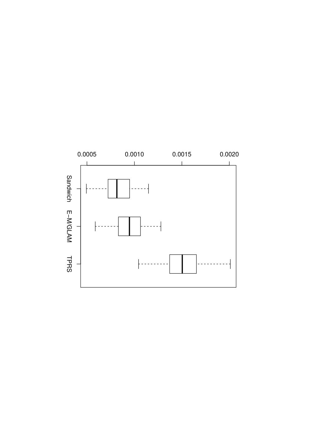
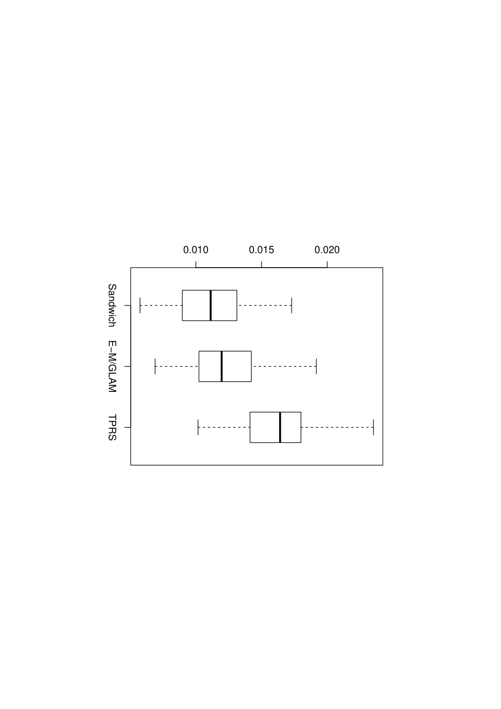
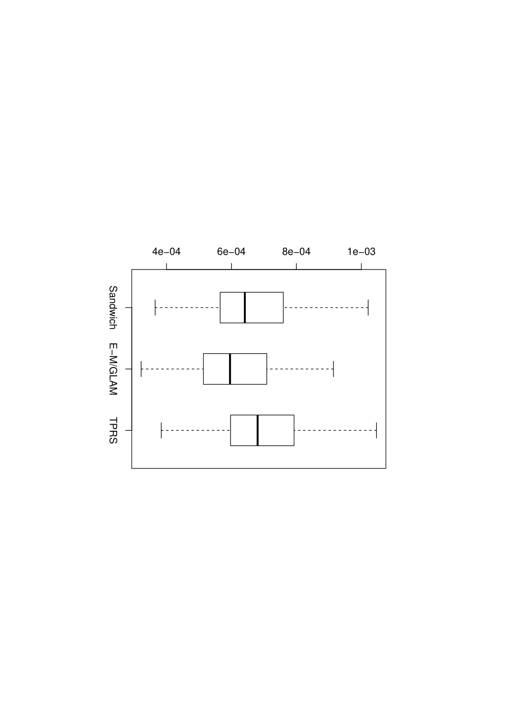
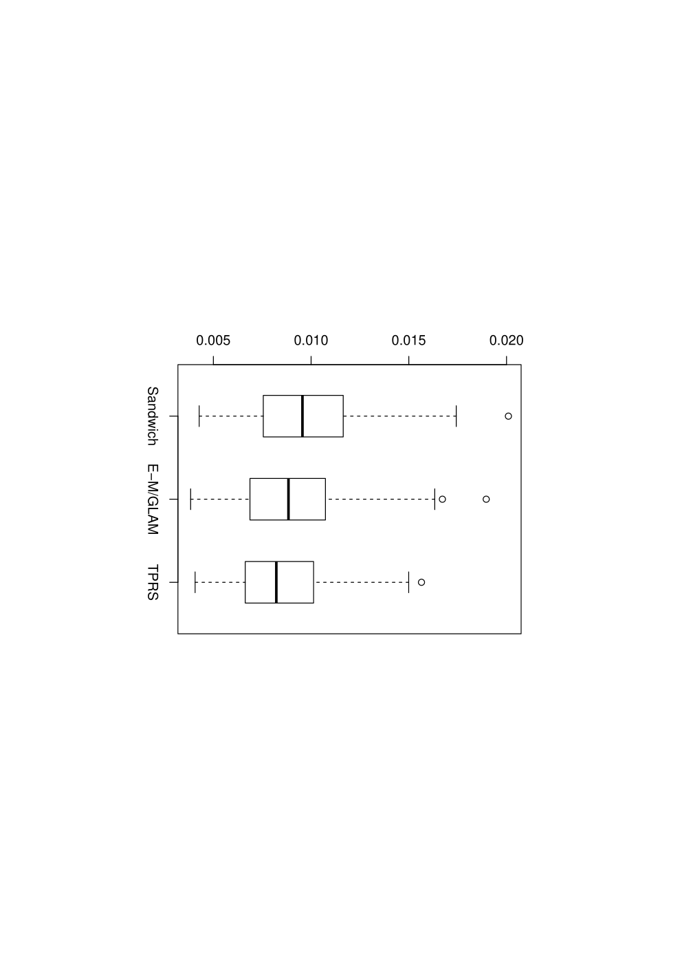
Performances of the three smoothers were assessed at two sample sizes. In the smaller sample study, each test function was sampled on the $20\times 30$ regular grid on the unit square, and random errors were iid $N(0,\sigma^{2})$ with $\sigma$ equal to 0.1 and 0.5. In each case, $100$ replicate data sets were generated and, for each replicate data, the test function was fitted by the three estimators and the integrated squared error (ISE) was calculated. For the spline basis and knots settings, based on the recommendation in Remark 3, $10$ and $15$ equidistant knots were used for the $x$ - and $z$ -axis for the two P-spline estimators. Thus, a total of 150 knots were used to construct the B-spline basis. Cubic B-splines were used with a second order difference penalty. For the thin plate regression estimator (TPRS), we implemented the TPRS using the function “bam” in a R package “mgcv” developed by Simon Wood. In this study, TPRS was used with a rank of 150 (i.e., the basis dimension is 150). For all three estimators, the smoothing parameters were chosen by GCV. The performances of the three estimators were evaluated by the mean ISEs (MISEs; see Table 1) and also boxplots of the ISEs (see Figure 2).

Table 1: MISEs of three estimators for a small sample size (data on a

20\times 30

grid).

$\sigma$ Sandwich smoother E-M/GLAM TPRS $f_{1}$ 0.1 $8.13\times 10^{-4}$ $9.29\times 10^{-4}$ $1.46\times 10^{-3}$ 0.5 $1.08\times 10^{-2}$ $1.18\times 10^{-2}$ $1.56\times 10^{-2}$ $f_{2}$ 0.1 $6.45\times 10^{-4}$ $5.73\times 10^{-4}$ $6.68\times 10^{-4}$ 0.5 $9.25\times 10^{-3}$ $8.34\times 10^{-3}$ $8.06\times 10^{-3}$

From Table 1 we can see that sandwich smoother did better than E-M/GLAM for estimating $f_{1}$ while E-M/GLAM was better for estimating $f_{2}$ . The boxplots in Figure 2 show that the two P-spline methods are essentially comparable. Compared to the two P-spline methods, TPRS gave larger MISEs except for one case. One explanation for the relative inferior performance of TPRS for estimating $f_{1}$ is that TPRS is isotropic and has only a single smoothing parameter so that the same amount of smoothing is applied in both directions, which might be not appropriate for $f_{1}$ as $f_{1}$ is quite smooth in $x$ and varies rapidly in $z$ (see Figure 1).

A larger sample simulation study with $n_{1}=60$ and $n_{2}=80$ was also done. For the two P-spline estimators, the numbers of knots were $K_{1}=30$ and $K_{2}=35$ . The rank of the TPRS was 1050, which was the total number of knots used in the two P-spline estimators. All the other settings were the same as in the smaller sample study. The resulting MISEs and boxplots gave the same conclusions as in the smaller sample study. To save space, we do not show the results here.

5.2 Computation speed

The computation speed of the three spline smoothers for smoothing $f_{2}$ with varying numbers of data points was assessed. For simplicity, we let $n_{1}=n_{2}$ and considered the case $\sigma=0.1$ . We selected the number of knots for the two P-spline smoothers following the recommendation in Remark 3. We fixed the rank of TPRS to the total number of knots used in the P-spline smoothers. For the two P-spline smoothers, the computation times reported are for the case where the search for optimal smoothing parameters is over a $20\times 20$ log scale grid in $[-5,4]^{2}$ . A finer grid with $40^{2}$ grid points was also used. The computation was done on 2.83GHz computers running Windows with 3GB of RAM. Table 2 summarizes the results and shows that the sandwich smoother is by far the fastest method. Note that the values in parenthesis are the computation time using the finer grid.

To further illustrate its computational capacity, the sandwich smoother was applied to large data with sizes of $300^{2}$ and $500^{2}$ . For cubic B-splines coupled with second-order difference penalty, Theorem 1 suggested choosing $K_{1}>n^{3/10}$ and $K_{2}>n^{3/10}$ . So we let $K_{1}=K_{2}$ with $K_{1}K_{2}$ close to $n^{3/5+0.1}$ in the simulations. We also evaluated the speed of E-M/GLAM. To save time, the E-M/GLAM was run for only $25$ pairs of smoothing parameters and the computation time was multiplied by 16 (64) so as to be comparable to that of the sandwich smoother on the coarse (fine) grid. The results in Table 2 show that the sandwich smoother could process large data quite fast on a personal computer while the E-M/GLAM is much slower. The TPRS was not applied to these large data as it would require more memory space than the computer could provide.

Table 2: Computation time (in seconds) of three estimators averaged over 100 data sets on 2.83GHz computers running Windows with 3GB of RAM. The times for the sandwich smoother and E-M/GLAM are for a

20\times 20

grid of smoothing parameter values and (in parenthesis) for a finer

40\times 40

grid. For

n=20^{2},40^{2}

and

80^{2}

, the number of knots for each axis is chosen by the recommendation in Remark 3. For

n=300^{2}

and

500^{2}

, the total number of knots for the sandwich smoother is approximately

n^{3/5+0.1}

as suggested by Theorem 1.

$n$ $K_{1}K_{2}$ Sandwich smoother E-M/GLAM TPRS $20^{2}$ $10^{2}$ 0.06(0.24) 4.09(19.74) 0.53 $40^{2}$ $20^{2}$ 0.08(0.30) 94.76(344.13) 19.50 $80^{2}$ $35^{2}$ 0.13(0.45) 1379.21(5487.33) 1032.07 $300^{2}$ $42^{2}$ 0.18(0.58) 3798.23(15192.92) – $500^{2}$ $57^{2}$ 0.32(0.89) 21023.44(84093.76) –

To summarize, the simulation study here and also the fast implementation in Section 2.2 show the advantage of the sandwich smoother over the two other estimators. So when computation time is of concern, the sandwich smoother might be preferred.

6 Application: covariance function estimation

As functional data analysis (FDA) has become a major research area, estimation of covariance functions has become an important application of bivariate smoothing. Because functional data sets can be quite large, fast calculation of bivariate smooths is essential in FDA, especially when the bootstrap is used for inference. Local polynomial smoothing is a popular method in estimating covariance functions (see e.g., Yao et al. (2005) or Yao and Lee (2006)) while other smoothing methods such as kernel (Staniswalis and Lee, 1998) and penalized splines (Di et al., 2009) have also been used. In this section, through a simulation study we compare the performance of the sandwich smoother and local polynomials for estimating a covariance function when the data are observed or measured at a fixed grid.

Let $\{X(t):t\in[0,1]\}$ be a stochastic process with a continuous covariance function $K(s,t)=\textrm{cov}\{X(s),X(t)\}$ . For simplicity, we assume $\textrm{E}X(t)=0,t\in[0,1]$ . Suppose $\{X_{i}(t),i=1,\dots,n\}$ is a collection of independent realizations of the above stochastic process and we observe the random functions $X_{i}$ at discrete design points with measurement errors,

Y_{ij}=X_{i}(t_{j})+\epsilon_{ij},1\leq j\leq J,1\leq i\leq n,

where $J$ is the number of measurements per curve, $n$ is the total number of curves, and the $\epsilon_{ij}$ are i.i.d. measurement errors with mean zero and finite variance and they are independent of the random functions $X_{i}$ . Let $\mathbf{Y}_{i}=(Y_{i1},\dots,Y_{iJ})^{T}$ . An estimate of the covariance function can be obtained through smoothing the sample covariance matrix $n^{-1}\sum_{i=1}^{n}\mathbf{Y}_{i}\mathbf{Y}_{i}^{T}$ by a bivariate smoother. Because we are smoothing a symmetric matrix, for the sandwich smoother we use two identical univariate smoother matrices so there is only one smoothing parameter to select. We use the commonly used local linear smoother (Yao et al., 2005, Hall et al., 2006) for comparison and the bandwidth is selected by the leave-one-curve-out cross validation. We wrote our own R implementation of the estimator used by Yao et al. (2005), since their code is in Matlab.

We let $K(s,t)=\sum_{k=1}^{4}\lambda_{k}\psi_{k}(s)\psi_{k}(t)$ where the eigenvalues $\lambda_{k}=0.5^{k-1},k=1,2,3,4$ , and $\{\psi_{1},\dots,\psi_{4}\}$ are the eigenfunctions from either of the following

	Case 1:	$\displaystyle\left\{\sqrt{2}\sin(2\pi t),\sqrt{2}\cos(2\pi t),\sqrt{2}\sin(4\pi t),\sqrt{2}\cos(4\pi t)\right\},$
	Case 2:	$\displaystyle\left\{1,\sqrt{3}(2t-1),\sqrt{5}(6t^{2}-6t+1),\sqrt{7}(20t^{3}-30t^{2}+12t-1)\right\}.$

The above two sets of eigenfunctions were used in Di et al. (2009), Greven et al. (2010), and Zipunnikov et al. (2011). We let $\sigma=0.5$ . We simulate 100 datasets and evaluate the two bivariate smoothers in terms of mean ISEs (MISEs). The results are given in Table 3. From Table 3, for case 1 with $(n,J)=(25,20)$ the local linear smoother is slightly better with smaller mean and standard deviation of ISE’s and for other cases the two smoothers give close results. The estimated eigenfunctions by the two smoothers for case 1 with $(n,J)=(25,20)$ are shown in Figure 3. The figure shows that both smoothers estimate the eigenfunctions well. We found similar results for $(n,J)=(100,40)$ (results not shown).

Table 3: MISEs of the sandwich smoother and the local linear smoother for estimating a covariance function. The number in parenthesis is the standard deviation of ISE’s.

$(n,J)$ Case Sandwich smoother Local linear smoother $(25,20)$ $1$ $.053(.035)$ $.050(.026)$ $2$ $.199(.139)$ $.204(.144)$ $(100,40)$ $1$ $.014(.008)$ $.013(.008)$ $2$ $.050(.034)$ $.050(.036)$

We also compared the computation time of the two smoothers using case 1 for various values of $J$ . For the sandwich smoother, we searched over twenty smoothing parameters. For the local linear smoother, we fixed the bandwidth. Note that selecting the bandwidth by the leave-one-curve-out cross validation means the computation time of the local linear smoother will be multiplied by the number of bandwidths and also the number of curves. Table 4 shows that the sandwich smoother is much faster to compute than the local linear smoother for covariance function estimation even when the bandwidth for the latter is fixed.

Table 4: Computation time (in seconds) for smoothing an

J\times J

covariance matrix using the sandwich smoother and the local linear smoother. With one exception, the computation times are averaged over 100 data sets on 2.83GHz computers running Windows with 3GB of RAM. The number of curves is fixed at 100. The bandwidth for the local linear smoother is fixed in the computations. The exception is that the computation time for the local linear smoother when

J=320

is averaged over 10 datasets only.

$J$ Sandwich smoother Local linear smoother $40$ 0.02 2.98 $80$ 0.03 50.04 $160$ 0.05 961.42 $320$ 0.16 13854.40

To summarize, the simulation study suggests that for covariance function estimation when functional data are measured at a fixed grid, the sandwich smoother is comparable to the local linear smoother in terms of MISEs. The sandwich smoother is considerably faster to compute than the local linear smoother.

7 Multivariate P-splines

We extend the sandwich smoother to array data of dimensions greater than two. Suppose we have a nonparametric regression model with $d\geq 3$ covariates

y_{i_{1},\dots,i_{d}}=\mu(x_{i_{1}},\dots,x_{i_{d}})+\epsilon_{i_{1},\dots,i_{d}},\quad 1\leq i_{k}\leq n_{k},1\leq k\leq d,

so the data are collected on a $d$ -dimensional grid. For simplicity, assume the covariates are in $[0,1]^{d}$ . As in the bivariate case, we model the $d$ -variate function $\mu(x_{1},\dots,x_{d})$ by tensor-product B-splines of $d$ variables $\sum_{\kappa_{1},\kappa_{2},\dots,\kappa_{d}}\theta_{\kappa_{1},\kappa_{2},\dots,\kappa_{d}}B_{\kappa_{1}}^{1}(x_{1})B_{\kappa_{2}}^{1}(x_{2})\cdots B_{\kappa_{d}}^{d}(x_{d}),$ where $B_{\kappa_{1}}^{1},B_{\kappa_{2}}^{2},\dots,B_{\kappa_{d}}^{d}$ are the B-spline basis functions. We smooth along all covariates simultaneously so that the fitted values and the data satisfy

\hat{\mathbf{y}}=\left(\mathbf{S}_{d}\otimes\mathbf{S}_{d-1}\otimes\dots\otimes\mathbf{S}_{1}\right)\mathbf{y},

(18)

where $\mathbf{S}_{i}$ is the smoother matrix for the $i$ th covariate using P-splines as in (3), $\mathbf{y}$ is the data vector organized first by $x_{1}$ , then by $x_{2}$ , and so on, and $\hat{\mathbf{y}}$ is organized the same way as $\mathbf{y}$ . Similar to equation (7), the estimate of coefficients $\hat{\boldsymbol{\theta}}$ satisfies

\left(\mathbf{\Lambda}_{d}\otimes\mathbf{\Lambda}_{d-1}\otimes\cdots\otimes\mathbf{\Lambda}_{1}\right)\hat{\boldsymbol{\theta}}=(\mathbf{B}_{d}\otimes\mathbf{B}_{d-1}\otimes\cdots\otimes\mathbf{B}_{1})^{T}\mathbf{y},

and the penalized estimate is

\hat{\mu}(x_{1},x_{2},\dots,x_{d})=\sum_{\kappa_{1},\kappa_{2},\dots,\kappa_{d}}\hat{\theta}_{\kappa_{1},\kappa_{2},\dots,\kappa_{d}}B_{\kappa_{1}}^{1}(x_{1})B_{\kappa_{2}}^{1}(x_{2})\cdots B_{\kappa_{d}}^{d}(x_{d}).

7.1 Implementation of the multivariate P-splines

Two computational issues occur for smoothing data on a multi-dimensional grid. The first issue is that unless the sizes of $\mathbf{S}_{i}$ ’s are all small, the storage and computation of $\mathbf{S}_{d}\otimes\mathbf{S}_{d-1}\otimes\dots\otimes\mathbf{S}_{1}$ will be challenging. The second issue is selection of smoothing parameters. Because of the large number of smoothing parameters involved, finding the smoothing parameters that minimize some model selection criteria such as GCV can be difficult.

The generalized linear array model by Currie et al. (2006) provided an elegant solution to the first issue by making use of the array structures of the model matrix as well as the data. The smoother matrix $\mathbf{S}_{d}\otimes\mathbf{S}_{d-1}\otimes\dots\otimes\mathbf{S}_{1}$ in multivariate smoothing has a tensor product structure, hence $\hat{\mathbf{y}}$ in (18) can be computed efficiently by a sequence of nested operations on $\mathbf{y}$ by the GLAM algorithm. For instance, consider $d=3$ . Then $\hat{\mathbf{y}}$ can be computed efficiently with one line of R code:

# The function "RH" is the rotated H-transform of an array by a matrix
# see Currie et al. (2006)
yhat = as.vector(RH(S3,RH(S2,RH(S1,Y))))

We wrote an R version of the RH function.

The second issue can be easily handled for the multivariate fast P-splines. Because of the tensor product structure of the smoother matrix, the fast implementation in Section 2.2 can be generalized for the multivariate case. As an illustration, we show how to compute the trace of the smoother matrix. We first compute the singular value decompositions for all $\mathbf{S}_{i}$ so that (13) holds for all $i=1,\dots,d$ , then we compute the trace of the smoother matrix by

{\rm tr}\left(\mathbf{S}_{d}\otimes\mathbf{S}_{d-1}\otimes\dots\otimes\mathbf{S}_{1}\right)=\prod_{i=1}^{d}{\rm tr}(\mathbf{S}_{i})

using the identity in (12) repeatedly. Note that ${\rm tr}(\mathbf{S}_{i})$ has a similar expression as in (13) for all $i$ .

The sandwich smoother does not have a GLM weight matrix and when it is used for bivariate smoothing, there is no need for rotation of arrays, so we do not consider the bivariate sandwich smoother to be a GLAM algorithm. However, our implementation for the bivariate sandwich smoother makes use of tensor product structures to simplify calculations similar to what the GLAM does.

7.2 An example

Smoothing simulated image data of size $128\times 128\times 24$ with a $20^{3}$ grid of smoothing parameters, the sandwich smoother takes about 20 seconds on a 2.4GHz computer running Mac software with 4GB of RAM. We have not found the computation time of other smoothers, but we can give a crude lower bound. We see in Table 2 that E-M/GLAM takes about 1400 seconds (over 20 minutes) on a $80^{2}$ two-dimensional grid where the smoothing parameters are searched over a $20\times 20$ grid. Searching over a $20\times 20\times 20$ grid to select the smoothing parameters, the number of times of GCV computation is now 20 times more. Moreover, for each GCV computation, E-M/GLAM will need much more time for smoothing data of size $128\times 128\times 24$ which is much larger. Therefore, the E-M/GLAM estimator’s computation time for smoothing a $128\times 128\times 24$ will be many hours for an algorithm that does not compute GCV as efficiently as the sandwich smoother does.

Acknowledgement

This research was partially supported by National Science Foundation grant DMS-0805975 and National Institutes of Health grant R01-NS060910. Luo Xiao’s research was partly supported by the National Center for Research Resources Grant UL1-RR024996. We thank Professor Iain Currie for his helpful discussion on the GLAM algorithm. We thank the two referees and the associate editor for their most helpful comments and suggestions which greatly improve this paper. We are grateful to one referee who suggested the name “sandwich smoother”.

Appendix A Appendix: Derivation of equation (11)

First we have

\|\hat{\mathbf{Y}}-\mathbf{Y}\|_{F}^{2}=(\hat{\mathbf{y}}-\mathbf{y})^{T}(\hat{\mathbf{y}}-\mathbf{y})=\hat{\mathbf{y}}^{T}\hat{\mathbf{y}}-2\hat{\mathbf{y}}^{T}\mathbf{y}+\mathbf{y}^{T}\mathbf{y}.

It can be shown by (10) that

\begin{split}\hat{\mathbf{y}}^{T}\hat{\mathbf{y}}&=\tilde{\mathbf{y}}^{T}(\boldsymbol{\Sigma}_{2}\otimes\boldsymbol{\Sigma}_{1})(\mathbf{A}_{2}\otimes\mathbf{A}_{1})^{T}(\mathbf{A}_{2}\otimes\mathbf{A}_{1})(\boldsymbol{\Sigma}_{2}\otimes\boldsymbol{\Sigma}_{1})\tilde{\mathbf{y}}\\ &=\tilde{\mathbf{y}}^{T}(\boldsymbol{\Sigma}_{2}\otimes\boldsymbol{\Sigma}_{1})(\boldsymbol{\Sigma}_{2}\otimes\boldsymbol{\Sigma}_{1})\tilde{\mathbf{y}}\\ &=|\tilde{\mathbf{y}}^{T}(\boldsymbol{\Sigma}_{2}\otimes\boldsymbol{\Sigma}_{1})|^{2}\\ &=\left\{\tilde{\mathbf{y}}^{T}\left(\tilde{\mathbf{s}}_{2}\otimes\tilde{\mathbf{s}}_{1}\right)\right\}^{2}.\end{split}

In the above derivation, $|\cdot|$ denotes the Euclidean norm in the second to last equality; we used the facts that $\mathbf{A}_{i}^{T}\mathbf{A}_{i}=\mathbf{I}_{c_{i}}$ and that both $\boldsymbol{\Sigma}_{2}$ and $\boldsymbol{\Sigma}_{1}$ are diagonal matrices. Similarly we obtain

\hat{\mathbf{y}}^{T}\mathbf{y}=\left\{\tilde{\mathbf{y}}^{T}\left(\tilde{\mathbf{s}}_{2}^{1/2}\otimes\tilde{\mathbf{s}}_{1}^{1/2}\right)\right\}^{2}

and hence establishes (11).

Appendix B Appendix: Proof of theorems

Lemma 1

The univariate kernel function $H_{m}(x)$ defined in (14) satisfies the following:

\int_{-\infty}^{\infty}x^{l}H_{m}(x)\,\mathrm{d}x=\begin{cases}1&:\quad l=0\\ 0&:\quad l\quad\mbox{is odd}\\ 0&:\quad l\quad\mbox{is even and }\quad 2\leq l\leq 2m-2\\ (-1)^{m+1}(2m)!&:\quad l=2m\end{cases}.

Hence $H_{m}(x)$ is of order $2m$ .

Proof of Lemma 1: We need to calculate two types of integrals $\int x^{l}\exp(ax)\cos(bx)\,\mathrm{d}x$ and $\int x^{l}\exp(ax)\sin(bx)\,\mathrm{d}x$ . Those indefinite integrals are given by results 3 and 4 in Gradshteyn and Ryzhik (2007, pp. 230). Then a routine calculation gives the desired result. Part of the lemma is derived in Wang et al. (2011). Details of derivation can be found in Xiao et al. (2011).

Before proving Proposition 1, we need the following lemma:

Lemma 2

Use the same notation in Proposition 1 and assume all conditions and assumptions in Proposition 1 are satisfied. For $(x,z)\in(0,1)\times(0,1)$ , there exists a constant $C>0$ such that

\hat{\mu}(x,z)=\sum_{i,j}y_{i,j}\left[\left\{\sum_{\kappa,r}B_{\kappa}^{1}(x)B_{r}^{1}(x_{i})S_{\kappa,r,x}\right\}\left\{\sum_{\ell,s}B_{\ell}^{2}(z)B_{s}^{2}(z_{j})S_{\ell,s,z}\right\}+\tilde{b}_{i,j}(x,z)\right],

where $\tilde{b}_{i,j}(x,z)=O\left[\exp\left\{-C\min(h_{n,1}^{-1},h_{n,2}^{-1})\right\}\right]$ .

Proof of Lemma 2: By (8), $\hat{\mu}(x,z)=\sum\hat{\theta}_{\kappa,\ell}B_{\kappa}^{1}(x)B_{\ell}^{2}(z)$ . We only need to consider $\hat{\theta}_{\kappa,\ell}$ for which $B_{\kappa}^{1}(x)$ and $B_{\ell}^{2}(z)$ are both non-zero. Hence assume $\kappa$ and $\ell$ satisfy $\kappa\in(K_{1}x-p_{1}-1,K_{1}x+p_{1}+1)$ , $\ell\in(K_{2}z-p_{2}-1,K_{2}z+p_{2}+1)$ . Let $q_{1}=\max(p_{1},m_{1})$ and $q_{2}=\max(p_{2},m_{2})$ . Denote by $\mathbf{\Lambda}_{1,j}$ the $j$ th column of $\mathbf{\Lambda}_{1}$ and $\mathbf{\Lambda}_{2,j}$ the $j$ th column of $\mathbf{\Lambda}_{2}$ . As shown in Xiao et al. (2011) and Li and Ruppert (2008), there exist vectors $\mathbf{S}_{\kappa,x}$ and a constant $C_{3}>0$ so that for $q_{1}<j<c_{1}-q_{1}$ , $\mathbf{S}_{\kappa,x}^{T}\mathbf{\Lambda}_{1,j}=\delta_{\kappa,j}$ , and for $1\leq j\leq q_{1}$ or $c_{1}-q_{1}\leq j\leq c_{1}$ , $\mathbf{S}_{\kappa,x}^{T}\mathbf{\Lambda}_{1,j}=O\left[\exp\left\{-C_{3}h_{n,1}^{-1}\min(x,1-x)\right\}\right]$ . Here $\delta_{\kappa,j}=1$ if $j=\kappa$ and $0$ otherwise. Similarly, there exist vectors $\mathbf{S}_{\ell,z}$ and a constant $C_{4}>0$ such that for $q_{2}<j<c_{2}-q_{2}$ , $\mathbf{S}_{\ell,z}^{T}\mathbf{\Lambda}_{2,j}=\delta_{\ell,j}$ , and for $1\leq j\leq q_{2}$ or $c_{2}-q_{2}\leq j\leq c_{2}$ , $\mathbf{S}_{\ell,z}^{T}\mathbf{\Lambda}_{2,j}=O\left[\exp\left\{-C_{4}h_{n,2}^{-1}\min(z,1-z)\right\}\right]$ . Let $\tilde{\theta}_{\kappa,\ell}=\left(\mathbf{S}_{\ell,z}\otimes\mathbf{S}_{\kappa,x}\right)^{T}\left(\mathbf{\Lambda}_{2}\otimes\mathbf{\Lambda}_{1}\right)\hat{\boldsymbol{\theta}}$ and $C=\min\left\{C_{3}\min(x,1-x),C_{4}\min(z,1-z)\right\}$ , then

\tilde{\theta}_{\kappa,\ell}-\hat{\theta}_{\kappa,\ell}=\sum_{i,j}\tilde{b}_{i,j,\kappa,\ell}y_{i,j},

(19)

where $\tilde{b}_{i,j,\kappa,\ell}=O\left[\exp\left\{-C\min(h_{n,1}^{-1},h_{n,2}^{-1})\right\}\right]$ . By equation (7),

\tilde{\theta}_{\kappa,\ell}=\left(\mathbf{S}_{\ell,z}\otimes\mathbf{S}_{\kappa,x}\right)^{T}\left(\mathbf{B}_{2}^{T}\otimes\mathbf{B}_{1}^{T}\right)\mathbf{y}=\left(\mathbf{S}_{\ell,z}^{T}\mathbf{B}_{2}^{T}\otimes\mathbf{S}_{\kappa,x}^{T}\mathbf{B}_{1}^{T}\right)\mathbf{y}=\mathbf{S}_{\kappa,x}^{T}\left(\mathbf{B}_{1}^{T}\mathbf{Y}\mathbf{B}_{2}\right)\mathbf{S}_{\ell,z}.

Letting $S_{\kappa,r,x}$ be the $r$ th element of $\mathbf{S}_{\kappa,x}$ and similarly $S_{\ell,s,z}$ the $s$ th element of $\mathbf{S}_{\ell,z}$ , we express $\tilde{\theta}_{\kappa,\ell}$ as a double sum

\tilde{\theta}_{\kappa,\ell}=\sum_{r,s}S_{\kappa,r,x}\left\{\sum_{i,j}B_{r}^{1}(x_{i})y_{i,j}B_{s}^{2}(z_{j})\right\}S_{\ell,s,z}=\sum_{i,j}y_{i,j}\left\{\sum_{r}B_{r}^{1}(x_{i})S_{\kappa,r,x}\right\}\left\{\sum_{s}B_{s}^{2}(z_{j})S_{\ell,s,z}\right\}.

(20)

With equations (8), (19) and (20), we have

\begin{split}\hat{\mu}(x,z)&=\sum_{\kappa,\ell}\tilde{\theta}_{\kappa,\ell}B_{\kappa}^{1}(x)B_{\ell}^{2}(z)+\sum_{\kappa,\ell}(\hat{\theta}_{\kappa,\ell}-\tilde{\theta}_{\kappa,\ell})B_{\kappa}^{1}(x)B_{\ell}^{2}(z)\\ &=\sum_{i,j}y_{i,j}\left[\left\{\sum_{\kappa,r}B_{\kappa}^{1}(x)B_{r}^{1}(x_{i})S_{\kappa,r,x}\right\}\left\{\sum_{\ell,s}B_{\ell}^{2}(z)B_{s}^{2}(z_{j})S_{\ell,s,z}\right\}+\tilde{b}_{i,j}(x,z)\right],\end{split}

where $\tilde{b}_{i,j}(x,z)=O\left[\exp\left\{-C\min(h_{n,1}^{-1},h_{n,2}^{-1})\right\}\right]$ .

Proof of Proposition 1: Let $\tilde{\lambda}_{1}=\lambda_{1}K_{1}n_{1}^{-1}=(K_{1}h_{n,1})^{2m_{1}}$ and $\tilde{\lambda}_{2}=\lambda_{2}K_{2}n_{2}^{-1}=(K_{2}h_{n,2})^{2m_{2}}$ . By Proposition 5.1 in Xiao et al. (2011), there exists some constants $0<\phi_{1},\phi_{2}<\infty$ such that

\begin{split}&n_{1}h_{n,1}\sum_{k,r}B_{k}^{1}(x)B_{r}^{1}(x_{i})S_{k,r,x}\\ =&H_{m_{1}}\left(\frac{|x-x_{i}|}{h_{n,1}}\right)+\delta_{\{p_{1}>m_{1}\}}\left[O\left(\tilde{\lambda}_{1}^{-2+\frac{1}{2m_{1}}}\right)+\delta_{\{|x-x_{i}|<\phi_{1}/K_{1}\}}O\left(\tilde{\lambda}_{1}^{-\frac{p_{1}}{p_{1}-m_{1}}+\frac{1}{2m_{1}}}\right)\right]\\ &+\exp\left(-\phi_{2}\frac{|x-x_{i}|}{h_{n,1}}\right)\left[O\left(\tilde{\lambda}_{1}^{-\frac{1}{m_{1}}}\right)+\delta_{\{m_{1}=1\}}\delta_{\left\{|x-x_{i}|\leq(p_{1}+1)\tilde{\lambda}_{1}^{-1/(2m_{1})}\right\}}O\left(\tilde{\lambda}_{1}^{-\frac{1}{2m_{1}}}\right)\right].\end{split}

(21)

Here $\delta_{\{p_{1}>m_{1}\}}=1$ if $p_{1}>m_{1}$ and 0 otherwise; the other $\delta$ terms are similarly defined. Similarly, there exist some constants $0<\phi_{3},\phi_{4}<\infty$ such that

\begin{split}&n_{2}h_{n,2}\sum_{\ell,s}B_{\ell}^{2}(z)B_{s}^{2}(z_{j})S_{\ell,s,z}\\ =&H_{m_{2}}\left(\frac{|z-z_{j}|}{h_{n,2}}\right)+\delta_{\{p_{2}>m_{2}\}}\left[O\left(\tilde{\lambda}_{2}^{-2+\frac{1}{2m_{2}}}\right)+\delta_{\{|z-z_{j}|<\phi_{3}/K_{2}\}}O\left(\tilde{\lambda}_{2}^{-\frac{p_{2}}{p_{2}-m_{2}}+\frac{1}{2m_{2}}}\right)\right]\\ &+\exp\left(-\phi_{4}\frac{|z-z_{j}|}{h_{n,2}}\right)\left[O\left(\tilde{\lambda}_{2}^{-\frac{1}{m_{2}}}\right)+\delta_{\{m_{2}=1\}}\delta_{\left\{|z-z_{j}|\leq(p_{2}+1)\tilde{\lambda}_{2}^{-1/(2m_{2})}\right\}}O\left(\tilde{\lambda}_{2}^{-\frac{1}{2m_{2}}}\right)\right].\end{split}

(22)

Let

	$\displaystyle d_{i,1}$	$\displaystyle=\sum_{k,r}B_{k}^{1}(x)B_{r}^{1}(x_{i})S_{k,r,x}-(n_{1}h_{n,1})^{-1}H_{m_{1}}\left\{h_{n,1}^{-1}(x-x_{i})\right\},$
	$\displaystyle d_{i,2}$	$\displaystyle=\sum_{\ell,s}B_{\ell}^{2}(z)B_{s}^{2}(z_{j})S_{\ell,s,z}-(n_{2}h_{n,2})^{-1}H_{m_{2}}\left\{h_{n,2}^{-1}(z-z_{j})\right\},$
	$\displaystyle b_{i,j}(x,z)$	$\displaystyle=\frac{1}{n_{1}h_{n,1}}H_{m_{1}}\left(\frac{\|x-x_{i}\|}{h_{n,1}}\right)d_{i,2}+\frac{1}{n_{2}h_{n,2}}H_{m_{2}}\left(\frac{\|z-z_{j}\|}{h_{n,2}}\right)d_{i,2}+d_{i,1}d_{i,2}+\tilde{b}_{i,j}(x,z).$

It follows from Lemma 2 that $\hat{\mu}(x,z)-\mu^{\ast}(x,z)=\sum_{i,j}b_{i,j}(x,z)y_{i,j}$ . Hence $\textrm{E}\{\hat{\mu}(x,z)-\mu^{\ast}(x,z)\}=\sum_{i,j}b_{i,j}(x,z)\mu(x_{i},z_{j})$ and $\textrm{var}\{\hat{\mu}(x,z)-\mu^{\ast}(x,z)\}=\sum_{i,j}b_{i,j}^{2}(x,z)\sigma^{2}(x_{i},z_{j})$ .

To simplify notation, denote $\max\{(K_{1}h_{n,1})^{-2},(K_{2}h_{n,2})^{-2}\}$ by $\xi$ . We prove $\textrm{E}\{\hat{\mu}(x,z)-\mu^{\ast}(x,z)\}=O(\xi)$ by showing that $\sum_{i,j}|b_{i,j}(x,z)\mu(x_{i},z_{j})|$ is $O(\xi)$ . By Lemma 2, $\tilde{b}_{i,j}(x,z)=O\left[\exp\left\{-C\min(h_{n,1}^{-1},h_{n,2}^{-1})\right\}\right]$ . Since $h_{n,1}=O(n^{-\nu_{1}})$ and $h_{n,2}=O(n^{-\nu_{2}})$ , $\tilde{b}_{i,j}(x,z)=n^{-1}o(\xi)$ and hence $\sum_{i,j}|\tilde{b}_{i,j}(x,z)\mu(x_{i},z_{j})|=o(\xi).$ For simplicity, we shall only show that

\sum_{i,j}\left|\frac{1}{n_{1}h_{n,1}}H_{m_{1}}\left(\frac{|x-x_{i}|}{h_{n,1}}\right)d_{i,2}\mu(x_{i},z_{j})\right|=O(\xi),

(23)

and we use the case when $p_{2}\leq m_{2}$ as an example. Because

		$\displaystyle\frac{1}{nh_{n}}\sum_{i,j}\left\|H_{m_{1}}\left(\frac{\|x-x_{i}\|}{h_{n,1}}\right)\exp\left(-\phi_{4}\frac{\|z-z_{j}\|}{h_{n,2}}\right)\mu(x_{i},z_{j})\right\|=O(1),$
		$\displaystyle\frac{1}{nh_{n}}\sum_{i,j}\left\|H_{m_{1}}\left(\frac{\|x-x_{i}\|}{h_{n,1}}\right)\exp\left(-\phi_{4}\frac{\|z-z_{j}\|}{h_{n,2}}\right)\delta_{\left\{\|z-z_{j}\|\leq(p_{2}+1)\tilde{\lambda}_{2}^{-1/(2m_{2})}\right\}}\mu(x_{i},z_{j})\right\|=O\left\{\tilde{\lambda}_{2}^{-\frac{1}{2m_{2}}}\right\},$

and $\tilde{\lambda}_{2}^{-1/m_{2}}=(K_{2}h_{n,2})^{-2}$ , equality (23) is proved. The case when $p_{2}>m_{2}$ and the desired results involving $d_{i,1}$ can be similarly proved.

Next we show that $\textrm{var}\{\hat{\mu}(x,z)-\mu^{\ast}(x,z)\}=o\{(nh_{n})^{-1}\}$ , i.e., $\sum_{i,j}b_{i,j}^{2}(x,z)\sigma^{2}(x_{i},z_{j})=o\{(nh_{n})^{-1}\}$ . Note that $b_{i,j}^{2}(x,z)\sigma^{2}(x_{i},z_{j})$ can be expanded into a sum of individual terms. With similar analysis as before, for each individual term in $b_{i,j}^{2}(x,z)\sigma^{2}(x_{i},z_{j})$ , the double sum over $i,j$ is either $O\{(nh_{n})^{-1}\tilde{\lambda}_{1}^{-2/m_{1}}\}$ , $O\{(nh_{n})^{-1}\tilde{\lambda}_{2}^{-2/m_{2}}\}$ , or is of smaller order.

Proof of Theorem 1: Proposition 1 states that the sandwich smoother is asymptotically equivalent to a kernel regression estimator with a product kernel $H_{m_{1}}(x)H_{m_{2}}(z)$ . To determine the asymptotic bias and variance of the kernel estimator, we conduct a similar analysis of multivariate kernel density estimator as in Wand and Jones (1995). By Proposition 1,

\textrm{E}\{\hat{\mu}(x,z)\}=\frac{1}{nh_{n,1}h_{n,2}}\sum_{i,j}\mu(x_{i},z_{j})H_{m_{1}}\left(\frac{x-x_{i}}{h_{n,1}}\right)H_{m_{2}}\left(\frac{z-z_{j}}{h_{n,2}}\right)+O(\xi),

(24)

where we continue using the notation $\xi=\max\{(K_{1}h_{n,1})^{-2},(K_{2}h_{n,2})^{-2}\}$ . Let

\begin{split}\mu_{0}(x,z)&=\frac{1}{nh_{n,1}h_{n,2}}\sum_{i,j}\mu(x_{i},z_{j})H_{m_{1}}\left(\frac{x-x_{i}}{h_{n,1}}\right)H_{m_{2}}\left(\frac{z-z_{j}}{h_{n,2}}\right)\\ &\,\,-\frac{1}{h_{n,1}h_{n,2}}\iint\mu(u,v)H_{m_{1}}\left(\frac{x-u}{h_{n,1}}\right)H_{m_{2}}\left(\frac{z-v}{h_{n,2}}\right)\mathrm{d}u\mathrm{d}v.\end{split}

(25)

The first term on the right hand of (25) is the Riemann finite sum of $(h_{n,1}h_{n,2})^{-1}\mu(u,v)$ $H_{m_{1}}\{h_{n,1}^{-1}(x-u)\}H_{m_{2}}\{h_{n,2}^{-1}(z-v)\}$ on the grid while the second term is the integral of the same function, and $\mu_{0}(x,z)$ calculates the difference between the two terms. $\mu_{0}(x,z)$ is not random and Lemma 4 shows that $\mu_{0}(x,z)=O\left\{\max\left(n_{1}^{-2}h_{n,1}^{-2},n_{2}^{-2}h_{n,2}^{-2}\right)\right\}$ . Now (24) becomes

	$\displaystyle\textrm{E}\left\{\hat{\mu}(x,z)\right\}$	$\displaystyle=\frac{1}{h_{n,1}h_{n,2}}\iint\mu(u,v)H_{m_{1}}\left(\frac{x-u}{h_{n,1}}\right)H_{m_{2}}\left(\frac{z-v}{h_{n,2}}\right)\mathrm{d}u\mathrm{d}v+\mu_{0}(x,z)+O(\xi)$
		$\displaystyle=\iint\mu(x-h_{n,1}u,z-h_{n,2}v)H_{m_{1}}(u)H_{m_{2}}(v)\mathrm{d}u\mathrm{d}v+\mu_{0}(x,z)+O(\xi).$		(26)

For the double integral in (26), we first take the Taylor expansion of $\mu(x-h_{n_{1}}u,z-h_{n_{2}}v)$ at $(x,z)$ until the $2m_{1}$ th partial derivative with respect to $x$ and the $2m_{2}$ th partial derivative with respect to $z$ , and then we cancel out those integrals that vanish by Lemma 1. It follows that explicit expressions for the asymptotic mean can be attained

	$\displaystyle\textrm{E}\left\{\hat{\mu}(x,z)\right\}-\mu(x,z)-\mu_{0}(x,z)$	$\displaystyle=(-1)^{m_{1}+1}h_{n,1}^{2m_{1}}\frac{\partial^{2m_{1}}}{\partial x^{2m_{1}}}\mu(x,z)+(-1)^{m_{2}+1}h_{n,2}^{2m_{2}}\frac{\partial^{2m_{2}}}{\partial z^{2m_{2}}}\mu(x,z)$
		$\displaystyle+o(h_{n,1}^{2m_{1}})+o(h_{n,2}^{2m_{2}})+O(\xi).$

For any two random variables $X$ and $Y$ , if $\textrm{var}(Y)=o\{\textrm{var}(X)\}$ , then $\textrm{var}(X+Y)=\textrm{var}(X)+o\{\textrm{var}(X)\}$ . Hence, by letting $X=\mu^{\ast}(x,z)$ and $Y=\hat{\mu}(x,z)-\mu^{\ast}(x,z)$ , we can obtain by Proposition 1 that

\displaystyle\textrm{var}\{\hat{\mu}(x,z)\}=(nh_{n})^{-1}\sigma^{2}(x,z)\int H_{m_{1}}^{2}(u)\mathrm{d}u\int H_{m_{2}}^{2}(v)\mathrm{d}v+o\{(nh_{n})^{-1}\}.

To get optimal rates of convergence, let $h_{n,1}^{2m_{1}}/h_{n,2}^{2m_{2}}$ and $h_{n,1}^{4m_{1}}/(nh_{n})^{-1}$ converge to some constants, repsectively. Then we have

\displaystyle h_{n,1}\sim h_{1}n^{-{m_{2}}/{m_{3}}},h_{n,2}\sim h_{2}n^{-{m_{1}}/{m_{3}}}

for some positive constants $h_{1}$ and $h_{2}$ . (Recall that $m_{3}=4m_{1}m_{2}+m_{1}+m_{2}$ .) We need to choose $K_{1},K_{2}$ so that $\max\{(K_{1}h_{n,1})^{-2},(K_{2}h_{n,2})^{-2}\}=o(h_{n,1}^{2m_{1}})$ . Hence, $K_{1}\sim C_{1}n^{\tau_{1}}$ for some positive constant $C_{1}$ and $\tau_{1}>(m_{1}m_{2}+m_{2})/m_{3}$ . Similarly, $K_{2}\sim C_{2}n^{\tau_{2}}$ for some positive constant $C_{2}$ and $\tau_{2}>(m_{1}m_{2}+m_{1})/m_{3}$ . It is easy to verify that $\max\left(n_{1}^{-2}h_{n,1}^{-2},n_{2}^{-2}h_{n,2}^{-2}\right)=o(h_{n,1}^{2m_{1}})$ .

Lemma 3

Let $G(x)$ be a real function in $[0,1]$ with a continuous second derivative. Let $x_{i}=(i-1/2)/n$ for $i=1,\dots,n$ . Assume $h=o(1),(nh^{2})^{-1}=o(1)$ as $n$ goes to infinity. Then

\left|\frac{1}{h}\int_{0}^{1}H_{m}\left(\frac{x-u}{h}\right)G(u)du-\frac{1}{nh}\sum_{i=1}^{n}H_{m}\left(\frac{x-x_{i}}{h}\right)G(x_{i})\right|=O(n^{-2}h^{-2}),

where $H_{m}(x)$ is defined in (14).

Proof of Lemma 3: First note that $H_{m}(x)$ is symmetric and is bounded by 1. Also $H_{m}(x)$ is infinitely differentiable over $(-\infty,0]$ and all the derivatives are bounded by $m$ over $(-\infty,0]$ . Let $L_{i}=[(i-1)/n,i/n]$ for $i=1,\dots,n$ . Suppose without loss of generality that $\max_{u\in[0,1]}|G(u)|\leq m$ . We have

\begin{split}&\left|\frac{1}{h}\int_{0}^{1}H_{m}\left(\frac{x-u}{h}\right)G(u)du-\frac{1}{nh}\sum_{i=1}^{n}H_{m}\left(\frac{x-x_{i}}{h}\right)G(x_{i})\right|\\ \leq&\sum_{i=1}^{n}\left|\frac{1}{h}\int_{L_{i}}\left\{H_{m}\left(\frac{x-u}{h}\right)G(u)-H_{m}\left(\frac{x-x_{i}}{h}\right)G(x_{i})\right\}du\right|,\end{split}

(27)

and

\begin{split}&\left|\frac{1}{h}\int_{L_{i}}\left\{H_{m}\left(\frac{x-u}{h}\right)G(u)-H_{m}\left(\frac{x-x_{i}}{h}\right)G(x_{i})\right\}du\right|\\ \leq&\left|\frac{G(x_{i})}{h}\int_{L_{i}}\left\{H_{m}\left(\frac{x-u}{h}\right)-H_{m}\left(\frac{x-x_{i}}{h}\right)\right\}du\right|+\left|\frac{1}{h}H_{m}\left(\frac{x-x_{i}}{h}\right)\int_{L_{i}}\left\{G(u)-G(x_{i})\right\}du\right|\\ &+\left|\frac{1}{h}\int_{L_{i}}\left\{H_{m}\left(\frac{x-u}{h}\right)-H_{m}\left(\frac{x-x_{i}}{h}\right)\right\}\left\{G(u)-G(x_{i})\right\}du\right|\\ \leq&m\left|\frac{1}{h}\int_{L_{i}}H_{m}\left(\frac{x-u}{h}\right)-H_{m}\left(\frac{x-x_{i}}{h}\right)du\right|+\frac{1}{h}\left|\int_{L_{i}}\left\{G(u)-G(x_{i})\right\}du\right|+O(n^{-3}h^{-2})\\ \leq&m\left|\frac{1}{h}\int_{L_{i}}\left\{H_{m}\left(\frac{x-u}{h}\right)-H_{m}\left(\frac{x-x_{i}}{h}\right)\right\}du\right|+O(n^{-3}h^{-1})+O(n^{-3}h^{-2}).\end{split}

(28)

In the derivation of (28), the term $O(n^{-3}h^{-1})$ follows from

\left|G(u)-G(x_{i})-(u-x_{i})\frac{\partial G}{\partial x}(x_{i})\right|\leq\frac{1}{2}(u-x_{i})^{2}\max_{0\leq x\leq 1}\left|\frac{\partial^{2}G}{\partial x^{2}}(x)\right|

and

\left|\int_{L_{i}}\left\{G(u)-G(x_{i})\right\}du\right|=\left|\int_{L_{i}}\left\{G(u)-G(x_{i})-(u-x_{i})\frac{\partial G}{\partial x}(x_{i})\right\}du\right|;

the term $O(n^{-3}h^{-2})$ follows from

\left|\frac{1}{h}\left\{H_{m}\left(\frac{x-u}{h}\right)-H_{m}\left(\frac{x-x_{i}}{h}\right)\right\}\left\{G(u)-G(x_{i})\right\}\right|=O(n^{-2}h^{-2})

since $|u-x_{i}|\leq n^{-1}$ when both $u$ and $x_{i}$ are in $L_{i}$ . Note that we used the equality $\int_{L_{i}}(u-x_{i})du=0$ in the above derivation and we shall use it later as well. Combining (27) and (28), we have

\begin{split}&\left|\frac{1}{h}\int_{0}^{1}H_{m}\left(\frac{x-u}{h}\right)G(u)du-\frac{1}{nh}\sum_{i=1}^{n}H_{m}\left(\frac{x-x_{i}}{h}\right)G(x_{i})\right|\\ \leq&m\sum_{i=1}^{n}\left|\frac{1}{h}\int_{L_{i}}\left\{H_{m}\left(\frac{x-u}{h}\right)-H_{m}\left(\frac{x-x_{i}}{h}\right)\right\}du\right|+O(n^{-2}h^{-2}).\end{split}

(29)

For simplicity, denote by $H_{m}^{(1)}(x)$ and $H_{m}^{(2)}(x)$ the first and second derivatives of $H_{m}(x)$ , respectively. Similarly, denote by $H_{m}^{(1)}(0)$ and $H_{m}^{(2)}(0)$ the right derivatives of $H_{m}(x)$ at 0. If $x\in L_{i}$ , then $H_{m}\left\{h^{-1}(x-u)\right\}-H_{m}\left\{h^{-1}(x-x_{i})\right\}=O(n^{-1}h^{-1})$ and hence

\left|\frac{1}{h}\int_{L_{i}}\left\{H_{m}\left(\frac{x-u}{h}\right)-H_{m}\left(\frac{x-x_{i}}{h}\right)\right\}du\right|=O(n^{-2}h^{-2}),\,\text{if}\,\,x\in L_{i}.

(30)

If $x<(i-1)/n$ , then $x\notin L_{i}$ . Let

\begin{split}\tilde{H}_{m}(u,x_{i},x,h)=&H_{m}\left(\frac{x-u}{h}\right)-H_{m}\left(\frac{x-x_{i}}{h}\right)-\frac{u-x_{i}}{h}H_{m}^{(1)}\left(\frac{x-x_{i}}{h}\right)\\ &-\frac{(u-x_{i})^{2}}{2h^{2}}H_{m}^{(2)}\left(\frac{x-x_{i}}{h}\right).\end{split}

Then $\tilde{H}_{m}(u,x_{i},x,h)=O(h^{-3}|u-x_{i}|^{3})$ . We have

	$\displaystyle\left\|\frac{1}{h}\int_{L_{i}}\left\{H_{m}\left(\frac{x-u}{h}\right)-H_{m}\left(\frac{x-x_{i}}{h}\right)\right\}du\right\|$
$\displaystyle=$	$\displaystyle\left\|\frac{1}{h}\int_{L_{i}}\left\{H_{m}\left(\frac{x-u}{h}\right)-H_{m}\left(\frac{x-x_{i}}{h}\right)-\frac{u-x_{i}}{h}H_{m}^{(1)}\left(\frac{x-x_{i}}{h}\right)\right\}du\right\|$
$\displaystyle\leq$	$\displaystyle\left\|\frac{1}{h}\int_{L_{i}}\frac{\left(u-x_{i}\right)^{2}}{2h^{2}}H_{m}^{(2)}\left(\frac{x-x_{i}}{h}\right)du\right\|+\left\|\frac{1}{h}\int_{L_{i}}\tilde{H}_{m}(u,x_{i},x,h)du\right\|$
$\displaystyle\leq$	$\displaystyle\frac{1}{2n^{2}h^{2}}\int_{L_{i}}\frac{1}{h}\left\|H_{m}^{(2)}\left(\frac{x-x_{i}}{h}\right)\right\|du+O(n^{-4}h^{-4}).$	(31)

We can similarly prove that (31) holds when $x>i/n$ . Now with (30) and (31),

\begin{split}&\sum_{i=1}^{n}\left|\frac{1}{h}\int_{L_{i}}\left\{H_{m}\left(\frac{x-u}{h}\right)-H_{m}\left(\frac{x-x_{i}}{h}\right)\right\}du\right|\\ \leq&\frac{1}{2n^{2}h^{2}}\int_{0}^{1}\frac{1}{h}\left|H_{m}^{(2)}\left(\frac{x-x_{i}}{h}\right)\right|du+O(n^{-3}h^{-4})+O(n^{-2}h^{-2}),\end{split}

which finishes the lemma.

Lemma 4

The term $\mu_{0}(x,z)$ defined in (25) is $O\left\{\max\left(n_{1}^{-2}h_{n,1}^{-2},n_{2}^{-2}h_{n,2}^{-2}\right)\right\}$ .

Proof of Lemma 4: To simplify notation, let $G_{2}(u,z)=h_{n,2}^{-1}\int_{0}^{1}H_{m_{2}}\{h_{n,2}^{-1}(z-v)\}\mu(u,v)dv$ and $G_{1}(u,z)=(n_{2}h_{n,2})^{-1}\sum_{j}H_{m_{2}}\{h_{n,2}^{-1}(z-z_{j})\}\mu(u,z_{j})-G_{2}(u,z)$ . Then $G_{1}$ is $O\{n_{2}^{-2}h_{n,2}^{-2}\}$ by Lemma 3. Note that $|\mu_{0}(x,z)|$ is bounded by the sum of

\left|\frac{1}{n_{1}h_{n,1}}\sum_{i}H_{m_{1}}\left(\frac{x-x_{i}}{h_{n,1}}\right)G_{1}(x_{i},z)\right|

(32)

and

\left|\frac{1}{n_{1}h_{n,1}}\sum_{j}H_{m_{1}}\left(\frac{x-x_{i}}{h_{n,1}}\right)G_{2}(x_{i},z)-\frac{1}{h_{n,1}}\int H_{m_{1}}\left(\frac{x-u}{h_{n,1}}\right)G_{2}(u,z)du\right|.

(33)

Because $G_{1}$ is $O\left(n_{2}^{-2}h_{n,2}^{-2}\right)$ , (32) is also $O\left(n_{2}^{-2}h_{n,2}^{-2}\right)$ . By Theorem 9.1 in the appendix of Durrett (2005), $\partial^{2}G_{2}/\partial u^{2}$ exists and is equal to $h_{n,2}^{-1}\int_{0}^{1}H_{m_{2}}\{h_{n,2}^{-1}(z-v)\}\partial^{2}\mu(u,v)/\partial u^{2}dv$ . Hence $\partial^{2}G_{2}/\partial u^{2}$ is continuous and bounded. Lemma 3 implies (33) is $O\left(n_{1}^{-2}h_{n,1}^{-2}\right)$ which finishes our proof.

Proof of Theorem 2: Denote the design points $\{x_{i},z_{i}\}_{i=1}^{n}$ by $(\underline{x},\underline{z})$ . Applying Lemma 2 and the proof of Proposition 1 to the binned data $\tilde{\mathbf{Y}}$ with $n_{1},n_{2}$ replaced by $I_{1},I_{2}$ , we obtain

	$\displaystyle\textrm{E}\left\{\hat{\mu}(x,z)\|(\underline{x},\underline{z})\right\}$	$\displaystyle=(Ih_{n})^{-1}\sum_{\kappa,\ell}\textrm{E}\left\{\tilde{y}_{\kappa,\ell}\|(\underline{x},\underline{z})\right\}G_{\kappa,\ell},$		(34)
	$\displaystyle\textrm{var}\left\{\hat{\mu}(x,z)\|(\underline{x},\underline{z})\right\}$	$\displaystyle=(Ih_{n})^{-2}\sum_{\kappa,\ell}\textrm{var}\left\{\tilde{y}_{\kappa,\ell}\|(\underline{x},\underline{z})\right\}G_{\kappa,\ell}^{2},$		(35)

where

G_{\kappa,\ell}=H_{m_{1}}\left(\frac{x-\tilde{x}_{\kappa}}{h_{n,1}}\right)H_{m_{2}}\left(\frac{z-\tilde{z}_{\ell}}{h_{n,2}}\right)+b_{\kappa,\ell}(x,z),

and $b_{\kappa,\ell}(x,z)$ is defined similarly to $b_{i,j}(x,z)$ in the proof of Proposition 1 with also $n_{1},n_{2}$ replaced by $I_{1},I_{2}$ . Let $n_{\kappa,\ell}$ be the number of data points in the $(\kappa,\ell)$ th bin. Then

\textrm{var}\left\{\tilde{y}_{\kappa,\ell}|(\underline{x},\underline{z})\right\}=n_{\kappa,\ell}^{-2}\sum_{i=1}^{n}\sigma^{2}(x_{i},z_{i})\delta_{\{|x_{i}-\tilde{x}_{\kappa}|\leq(2I_{1})^{-1},|z_{i}-\tilde{z}_{\ell}|\leq(2I_{2})^{-1}\}}.

So $\textrm{var}\left\{\sqrt{n_{\kappa,\ell}}\tilde{y}_{\kappa,\ell}|(\underline{x},\underline{z})\right\}$ is a Nadaraya-Watson kernel regression estimator of the conditional variance function $\sigma^{2}(x,z)$ at $(\tilde{x}_{\kappa},\tilde{z}_{\ell})$ . Similarly, we can show $n_{\kappa,\ell}/(nI^{-1})$ is a kernel density estimator of $f(x,z)$ at $(\tilde{x}_{\kappa},\tilde{z}_{\ell})$ . By the uniform convergence theory for kernel density estimators and Nadaraya-Watson kernel regression estimators (see, for instance, Hansen (2008)),

\sup_{\kappa,\ell}\left|n_{\kappa,\ell}/(nI^{-1})-f(\tilde{x}_{\kappa},\tilde{z}_{\ell})\right|=O_{p}\left\{\sqrt{I\ln n/n}+I^{-2}\right\}=o_{p}(1),

(36)

and

\sup_{\kappa,\ell}\left|\text{var}\left\{\sqrt{n_{\kappa,\ell}}\tilde{y}_{\kappa,\ell}|(\underline{x},\underline{z})\right\}-\sigma^{2}(\tilde{x}_{\kappa},\tilde{z}_{\ell})\right|=O_{p}\left\{\sqrt{I\ln n/n}+I^{-2}\right\}=o_{p}(1).

It follows by the above two equalities that

\sup_{\kappa,\ell}\left|\frac{n}{I}\text{var}\left\{\tilde{y}_{\kappa,\ell}|(\underline{x},\underline{z})\right\}-\frac{\sigma^{2}(\tilde{x}_{\kappa},\tilde{z}_{\ell})}{f(\tilde{x}_{\kappa},\tilde{z}_{\ell})}\right|=o_{p}(1).

(37)

By an argument similar to one in the proof of Proposition 1, for any continuous function $g(x,z)$ over $[0,1]^{2}$ , we can derive that

\frac{1}{Ih_{n}}\sum_{\kappa,\ell}g(\tilde{x}_{\kappa},\tilde{z}_{\ell})G^{2}_{\kappa,\ell}=g(x,z)\int H_{m_{1}}^{2}(u)du\int H_{m_{2}}^{2}(v)dv+o(1).

(38)

Then by equalities (35) and (37),

\left|\textrm{var}\left\{\hat{\mu}(x,z)|(\underline{x},\underline{z})\right\}-\frac{1}{nh_{n}Ih_{n}}\sum_{\kappa,\ell}\frac{\sigma^{2}(\tilde{x}_{\kappa},\tilde{z}_{\ell})}{f(\tilde{x}_{\kappa},\tilde{z}_{\ell})}G^{2}_{\kappa,\ell}\right|=\frac{o_{p}(1)}{nh_{n}Ih_{n}}\sum_{\kappa,\ell}G_{\kappa,\ell}^{2}=o_{p}\{(nh_{n})^{-1}\}.

(39)

By letting $g(x,z)=\sigma^{2}(x,z)/f(x,z)$ in (38), we derive from (39) that

\textrm{var}\left\{\hat{\mu}(x,z)|(\underline{x},\underline{z})\right\}=\frac{1}{nh_{n}}\frac{V(x,z)}{f(x,z)}+o_{p}\{(nh_{n})^{-1}\},

(40)

where $V(x,z)$ is defined in (17). We can write $\textrm{E}\left\{\tilde{y}_{\kappa,\ell}|(\underline{x},\underline{z})\right\}$ as

\textrm{E}\left\{\tilde{y}_{\kappa,\ell}|(\underline{x},\underline{z})\right\}=(n_{\kappa,\ell})^{-1}\sum_{i=1}^{n}\mu(x_{i},z_{i})\delta_{\{|x_{i}-\tilde{x}_{\kappa}|\leq(2I_{1})^{-1},|z_{i}-\tilde{z}_{\ell}|\leq(2I_{2})^{-1}\}}.

Equality (36) implies each bin is nonempty, so by taking a Taylor expansion of $\mu(x_{i},z_{j})$ at $(\tilde{x}_{\kappa},\tilde{z}_{\ell})$ we derive from the above equation that

\sup_{\kappa,\ell}\left|\textrm{E}\left\{\tilde{y}_{\kappa,\ell}|(\underline{x},\underline{z})\right\}-\mu(\tilde{x}_{\kappa},\tilde{z}_{\ell})\right|=O_{p}(I^{-1/2}).

It follows by equality (34) that

\displaystyle\left|\textrm{E}\left\{\hat{\mu}(x,z)|(\underline{x},\underline{z})\right\}-\frac{1}{Ih_{n}}\sum_{\kappa,\ell}\mu(\tilde{x}_{\kappa},\tilde{z}_{\ell})G_{\kappa,\ell}\right|=O_{p}(I^{-1/2})\frac{1}{Ih_{n}}\sum_{\kappa,\ell}|G_{\kappa,\ell}|=O_{p}(I^{-1/2}).

(41)

It is easy to show that

\frac{1}{Ih_{n}}\sum_{\kappa,\ell}\mu(\tilde{x}_{\kappa},\tilde{z}_{\ell})G_{\kappa,\ell}=\mu(x,z)+n^{-(2m_{1}2m_{2})/m_{3}}\tilde{\mu}(x,z)+o\left\{n^{-(2m_{1}2m_{2})/m_{3}}\right\},

where $\tilde{\mu}(x,z)$ is defined in (16). In light of equality (41) and the assumption that $I\sim c_{I}n^{\tau}$ with $\tau>(4m_{1}m_{2})/m_{3}$ ,

\textrm{E}\left\{\hat{\mu}(x,z)|(\underline{x},\underline{z})\right\}=\mu(x,z)+n^{-(2m_{1}2m_{2})/m_{3}}\tilde{\mu}(x,z)+o_{p}\left\{n^{-(2m_{1}2m_{2})/m_{3}}\right\}.

(42)

With (40) and (42), we can show that

n^{(2m_{1}2m_{2})/m_{3}}\left[\hat{\mu}(x,z)-\textrm{E}\left\{\hat{\mu}(x,z)|(\underline{x},\underline{z})\right\}\right]\Rightarrow N\left\{0,V(x,z)/f(x,z)\right\}

(43)

in distribution and

n^{(2m_{1}2m_{2})/m_{3}}\left[\textrm{E}\left\{\hat{\mu}(x,z)|(\underline{x},\underline{z})\right\}-\mu(x,z)\right]=\tilde{\mu}(x,z)+o_{p}(1).

(44)

Equalities (43) and (44) together prove the theorem.

References

: Claeskens, G., Krivobokova, T., and Opsomer, J. D. (2009), “Asymptotic properties of penalized spline estimators,” Biometrika, 96, 529-544.
: Currie, I.D., Durban, M. and Eilers, P.H.C. (2006), “Generalized linear array models with applications to multidimensional smoothing,” J. R. Statist. Soc. B, 68, 259-280.
: Di, C., Crainiceanu, C. M., Caffo, B. S., and Punjabi, N. (2009), “Multilevel functional principal component analysis,” Ann. Appl. Statist., 3, 458-488.
: Dierckx, P. (1982), “A fast algorithm for smoothing data on a rectangular grid while using spline functions,” SIAM J. Numer. Anal., 19, 1286-1304.
: Dierckx, P. (1995), Curve and Surface Fitting with Splines, Clarendon Press, Oxford.
: Durrett, R. (2005), Probability: Theory and Examples, Third Edition, Thomson.
: Eilers, P.H.C., Currie I.D. and Durban M. (2006), “Fast and compact smoothing on large multidimensional grids,” Comput. Statist. Data Anal., 50, 61-76.
: Eilers, P.H.C. and Goeman, J.J. (2004), “Enhancing scatterplots with smoothed densities,” Bioinformatics, 20, 623-628.
: Eilers, P.H.C. and Marx, B.D. (1996), “Flexbile smoothing with B-splines and penalties (with Discussion),” Statist. Sci., 11, 89-121.
: Eilers, P.H.C. and Marx, B.D. (2003), “Mulitvariate calibration with temperature interaction using two-dimensional penalized signal regression,” Chemometrics and Intelligent Laboratory Systems, 66, 159-174.
: Gradshteyn, I.S. and Ryzhik, I.M.(2007), Table of Integrals, Series, and Products, New York: Academic Press.
: Greven, S., Crainiceanu, C., Caffo, B. and Reich, D. (2010), “Longitudinal functional principal component,” Electronic J. Statist., 4, 1022-1054.
: Gu, C. (2002), Smoothing Spline ANOVA Models, New York: Springer.
: Hall, P., Müller, H.G., and Wang, J.L. (2006), “Properties of principal component methods for functional and longitudinal data analysis,” Ann. Statist., 34, 1493-1517.
: Hansen, B.E. (2008), “Uniform convergence rates for kernel estimation with dependent data,” Econometric Theory, 24, 726-748.
: Hastie, T. and Tibshirani, R.(1993), “Varying-coefficients models,” J. R. Statist. Soc. B, 55, 757-796.
: Laub, A.J.(2005), Matrix Analysis for Scientists and Engineers, SIAM.
: Kauermann, G., Krivobokova, T. and Fahrmeir, L. (2009), “Some asymptotic results on generalized penalized spline smoothing,” J. R. Statist. Soc. B, 71, 487-503.
: Li,Y. and Ruppert D. (2008), “On the asymptotics of penalized splines,” Biometrika, 95, 415-436.
: Marx, B.D. and Eilers, P.H.C. (2005), “Multdimensional Penalized Signal Regression,” Technometrics, 47, 13-22.
: Opsomer, J.D. and Hall, P. (2005), “Theory for penalised spline regression,” Biometrika, 95, 417-436.
: Ruppert, D. (2002), “Selecting the number of knots for penalized splines,” J. Comput. Graph. Statist., 1, 735-757.
: Ruppert, D., Wand, M.P. and Carroll, R.J. (2003), Semiparametric Regression, Cambridge: Cambridge University Press.
: Seber, G.A.F. (2007), A Matrix Handbook for Statisticians, New Jersey: Wiley-Interscience.
: Staniswalis, J.G. and Lee, J.J. (1998), “Nonparametric regression analysis of longitudinal data,” J. Amer. Statist. Assoc., 93, 1403-1418.
: Stone, C.J. (1980), “Optimial rates of convergence for nonparametric estimators,” Ann. Statist., 8, 1348-1360.
: Wand, M.P. and Jones, M.C. (1995), Kernel Smoothing, London: Chapman &Hall.
: Wang, X., Shen, J. and Ruppert, D. (2011), “Local Asymptotics of P-spline Smoothing,” Electronic J. Statist., 4, 1-17.
: Wood, S.N. (2003), “Thin plate regression splines,” J. R. Statist. Soc. B, 65, 95-114.
: Wood, S.N. (2006), Generalized additive models: an introduction with R, London: Chapman &Hall.
: Xiao, L., Li, Y., Apanasovich, T.V. and Ruppert, D. (2011), “Local asymptotics of P-splines,” available at http://arxiv.org/abs/1201.0708v3.
: Yao, F. and Lee C.M. (2006), “Penalized spline models for functional principal component analysis,” J. R. Statist. Soc. B, 68, 3-25.
: Yao, F., Müller, H.G., and Wang, J.L. (2005), “Functional data analysis for sparse longitudinal data,” J. Amer. Statist. Assoc., 100, 577-590.
: Zipunnikov, V., Caffo, B. S., Crainiceanu, C. M., Yousem D.M., Davatzikos, C., and Schwartz, B.S. (2011), “Multilevel functional principal component analysis for high-dimensional data,” J. Comput. Graph. Statist., 20(4), 852-873.

	$\displaystyle\textrm{E}\left\{\hat{\mu}(x,z)\|(\underline{x},\underline{z})\right\}$	$\displaystyle=(Ih_{n})^{-1}\sum_{\kappa,\ell}\textrm{E}\left\{\tilde{y}_{\kappa,\ell}\|(\underline{x},\underline{z})\right\}G_{\kappa,\ell},$		(34)
	$\displaystyle\textrm{var}\left\{\hat{\mu}(x,z)\|(\underline{x},\underline{z})\right\}$	$\displaystyle=(Ih_{n})^{-2}\sum_{\kappa,\ell}\textrm{var}\left\{\tilde{y}_{\kappa,\ell}\|(\underline{x},\underline{z})\right\}G_{\kappa,\ell}^{2},$		(35)